11.exploring the link between poverty pollution-population (0003www.iiste.org call for-paper_ps)

Journal of Economics and Sustainable Development www.iiste.org
ISSN 2222-1700 (Paper) ISSN 2222-2855 (Online)
Vol.2, No.11&12, 2011

Exploring the Link between Poverty-Pollution-Population (3Ps)
in Pakistan: Time Series Evidence
Khalid Zaman1 Dr. Iqtidar Ali Shah1*, Muhammad Mushtaq Khan1 , Mehboob Ahmad2

1. Department of Management Sciences, COMSATS Institute of Information Technology, Abbottabad, Pakistan
2. Department of Management Sciences, Bahria University, Islamabad, Pakistan.
∗ iqtidar@ciit.net.pk

Abstract
The relationship between poverty, population growth and environment has been widely debated inside the
academic circles. There is a general consensus that poverty is a major cause of population growth and
environmental degradation and reversely population growth is the major cause of poverty and
environmental degradation. The present study examines the impact of poverty on environment (air
pollution) and population and reversely the impact of population on environment (air pollution) and poverty
in the specific context of Pakistan during a period of 1975-2009. Data is analyzed using Ordinary Least
Square (OLS) regression method and Autoregressive Distributed Lag (ARDL)-bounds testing approach to
examine the linkage.
The results of the OLS test show that rapid population and air pollution has a significant contributor to
poverty in Pakistan. However, the results nullify the conventional view that poverty is a major cause of
environmental degradation (or air pollution), while the result supports the hypothesis that population have a
deleterious impact on increasing poverty. The results of bounds test show that there is a stable long-run
relationship between population, poverty and pollution in Pakistan. On the other hand, results of the
causality test show that there is a unidirectional causal flow from population to carbon dioxide emission.
The post reform period is observed with the estimated coefficient of the poverty dummy variable
(POVDUM) which shows that poverty in Pakistan has increased due to deprived performance of federal
policies on pro-poor reforms in Pakistan. The post reform period is observed with the population dummy
variable (POPDUM) reflecting that population growth has increased significantly during the said reform
period.
Keywords: Population, Air Pollution, Poverty, Headcount Ratio, Population Dynamics, Carbon Dioxide
Emission, Time Series, Bounds Test, Pakistan.

1. Introduction
There is a link exists between poverty-pollution-population and it has been focused in the literature. The
relationship between these variables is very complicated. However, a simple equation is that larger
population leads to more poverty and pollution and reversely, more poverty increased population and
pollution. The available global data suggest that all the three variables have been increasing worldwide.
Poverty is a complex phenomenon and besides other factors such as bad governance, income inequality and
weak economic growth; rapid population growth is the main contributor responsible for poverty. Poverty in
Pakistan has historically been elevated in rural than urban areas. Poverty rose more harshly in the rural
areas in the 1990s, and in 1999 the prevalence of rural poverty (36.3 percent) was significantly higher than
urban poverty (22.6 percent). According to the latest estimates, poverty head count ratio was 29.2 percent
in 2004-05 which increased to 33.8 percent in 2007-08 and 36.1 percent in 2008-09. About 62 million
people are below the poverty line during 2008-09 (GoP, 2009). The overall picture of poverty at national
level during the 1964-2006 is given in table 1, while figure 1 shows poverty statistics at rural, urban and at
national level of Pakistan during 1979-2006.
27 | P a g e
www.iiste.org

Vol.2, No.11&12, 2011

Environmental challenges and issues of Pakistan are associated primarily with an imbalanced social and
economic development from the last two to three decades. This challenge is further compounded with rapid
urbanization due to a shift of population from rural to urban areas. Thus, all major cities of Pakistan face
haphazard, unplanned expansion leading to increase in pollution. Main factors causing degradation to air
quality are, a) rapidly growing energy demand and b) a fast growing transport sector. In the cities,
widespread use of low quality fuel, combined with a dramatic expansion in the number of vehicles on roads,
has led to significant air pollution problems. Air pollution levels in Pakistan’s most populated cities are
high and climbing causing serious health issues. Although Pakistan’s energy consumption is still low by
world standards, but lead and carbon emissions are major air pollutants in urban centres (GoP, 2010).
Environmental degradation is fundamentally linked to poverty in Pakistan. Poverty is the main impediment
in dealing with the environment related problems. Environment generally refers to a natural-resource base
that provides sources (material, energy, and so forth) and performs “sink” functions (such as absorbing
pollution). The term can include resources that people relied on them in the past but no longer rely on
(either because they are depleted or because they have been substituted by some other resource or
technology). Similarly, it can include resources that people do not yet use, but could use with a change in
knowledge or technology (Leach and Mearns, 1991).
Poverty combined with a rapidly increasing population and growing urbanization, is leading to intense
pressures on the environment. This environment-poverty nexus cannot be ignored if effective and practical
solutions to remedy environmental hazards are to be taken. Therefore, there has been a dire need to work on
poverty alleviation. Pakistan is the world’s sixth most populous country. With an estimated population of
169.9 million as at end-June 2009, and an annual growth rate (revised) of 2.05 percent, it is expected that
Pakistan will become the fourth largest nation on earth in population terms by 2050.With a median age of
around 20 years; Pakistan is also a “young” country. It is estimated that there are currently approximately
104 million Pakistanis below the age of 30 years. Total working age population is 121.01 million, with the
size of the employed labor force estimated at 52.71 million as of 2008-09 (GoP, 2010). Due to declines in
mortality that began in the 1950s and the consistently high fertility levels of more than 6 births per woman
that lasted around 40 years, Pakistan’s population growth rate reached a high 3.2 percent by the end of the
1980s, after which it began to decline (see table 2). Pakistan’s population of 41 million in 1950 doubled to
around 82 million by 1980 and by 2005 had doubled again to around 160 million (UN, 2009).
The above discussion confirms a strong linkage between poverty, population and pollution (3 P’s) in
Pakistan. In this paper an analysis has been carried out to find a statistical relationship between 3 P’s in
Pakistan using secondary data from 1975-2009. This paper does not include all dimensions and factors of
the poverty-population-pollution problem but limited to the following variables:
• Poverty: According to Duraiappah (1996) there are two types of poverty: indigenous poverty is
poverty caused by environmental degradation while exogenous poverty is poverty caused by factors
other than environmental degradation. In this study both types of poverty were taken into account
which is represented by HCR (Head Count Ratio)
• Population: According to Marcoux (1999), there is a sharp variance between two main ideas:
stabilizing population to protect the environment and slowing population growth to foster rapid
economic growth. The problem is that economic growth even coupled with slower population
growth or even population stabilization, brings about greater environmental damage, other things
being equal. In this study population growth is taken into account which is represented by POP.
• Pollution: According to the United Nations International Strategy for Disaster Reduction (UNISDR,
2004) environmental degradation is defined as, the reduction of the capacity of the environment to
meet social and ecological objectives, and needs. Potential effects are varied and may contribute to
an increase in vulnerability and the frequency and intensity of natural hazards. Some examples are:
land degradation, deforestation, desertification, wild land fires, loss of biodiversity, land, water and
air pollution, climate change, sea level rise and ozone depletion. In this study only carbon dioxide
emission was taken into account for the proxy of air pollution which is represented by CO2.
The objective of this paper is to analyze the link between Poverty-Pollution-Population over the period of
28 | P a g e
www.iiste.org

Vol.2, No.11&12, 2011

1975-2009. More specific objectives are to find out:
• The impact of poverty on air pollution and population in the long and short run and
• The impact of population on air pollution and poverty in the long and short run.
The paper is organized as follows: after introduction which is provided in Section 1, literature review is
carried out in Section 2. Methodological framework is explained in Section 3. The estimation and
interpretation of results is mentioned in Section 4. Section 5 concludes the paper.

2. Literature Review
The relationship between poverty-environment and population-environment has been extensively explored
in the past. But relatively few researchers have examined the relationship between
poverty-pollution-population concurrently of a developing country like Pakistan. The relationship between
poverty and environmental degradation has been widely debated inside the academic circles. There is a
general consensus that poverty is a major cause of environmental degradation and environmental
degradation caused poverty (Zaman et al, 2010). There are different views on population-environment
linkages, Mishra (1995); Marcoux (1994) and Bojo and Reddy (2001) all have emphasis the need to slow
down population growth for the sake of enabling more productive investment and a higher rate of economic
growth. There seems to be three lines of well established empirical research areas dealing with poverty,
population and environmental degradation nexus. The first line of research mainly focuses on the
relationship between the poverty and environmental degradation.

2.1. Poverty and Environmental Degradation Nexus
The assumption of a vicious circle relationship between poverty and environmental degradation in
developing countries has long prevailed in the debate on poverty–environment linkages. The assumptions
were first launched in the report of the World Commission on Environment and Development (WCED,
1987) called Brundtland report and has later been echoed by a wide range of organizations (e.g., Durning,
1989; UNEP, 1995; World Bank, 1992).
According to Duraiappah (1998),
"There is much controversy surrounding the poverty-environmental degradation nexus. The
predominant school of thought argues that poverty is a major cause of environmental
degradation and if policy makers want to address environmental issues, then they must first
address the poverty problem. Another school of thought argues that a direct link between
poverty and environmental degradation is too simplistic and the nexus is governed by a
complex web of factors (p.2169)”.
Dasgupta and Moeler (1994) opine that economic growth and development can increase with
environmental problems. They create an index of real net national product (NNP) which takes into account
deprecation of the natural resource base. The authors believe that this index may replace traditional
measures of economic growth. Ravnborg (2003) examines five environmentally harmful natural resource
management practices in the Nicaraguan hillsides. The result does not support the hypothesis that poverty is
a major cause of environmental degradation. The result further shows that the immediate agents of
environmental degradation are the non-poor farmers, not the poorest. Scherr (2000) examine the downward
spiral i.e., negative relationship between poverty and natural resource degradation. According to him,
“The main strategies to jointly address poverty and environmental improvement are to
increase poor people's access to natural resources, enhance the productivity of poor people's
natural resource assets and involve local people in resolving public natural resource
management concerns” (Scherr, 2000, p.479).
Zaman et al (2010, a) empirically investigate the relationship between agriculture environment and rural
poverty in the context of Pakistan by using co-integration and Granger causality over 1980-2009. The
29 | P a g e
www.iiste.org

Vol.2, No.11&12, 2011

results find that there is unidirectional casual relationship between rural poverty and agriculture
environment in Pakistan. Yusuf (2004) pointed out that there are many things working in between in the
linkage from poverty to environmental degradation. Some of important ones include the population growth,
discount rate, low investment base resources and property right. Thus, according to Yusuf (2004), the
linkages between poverty and environment degradation is not so simple to blame poor for environmental
degradation. Khan and Khan (2009) contribute to the debate on the links between poverty and forestry
degradation by using the case of the forest rich Swat district, Pakistan. The result does not find empirical
support for the poverty–environment nexus.
Khan and Naqvi (2000) qualitatively analyzed the relationship between poverty and resource degradation in
Pakistan and found that the poor are the most vulnerable to ecological degradation and yet, the absence of
basic subsistence makes them predators of natural resources thereby further exacerbating their vulnerability.
They argue that the poverty–resource degradation link reflects unavoidable responses. Khan (2009)
estimates income and price elasticities of demand for improved environmental quality of two National
Parks in Northern Pakistan. The study concludes that environmental improvements are more beneficial to
low-income groups than for high-income groups. Aggrey et al (2010) explored the casual relationship
between poverty and environmental problems at the district level using econometric analysis in Katanga
basin in Uganda. The results of the study show that there is strong correlation of poverty with
environmental degradations. Deforestation and wet land degradation have positive relationship with poverty.
The results concluded that the welfare of poor districts in Katanga basin would see to be most significant.

2.2. Population and Environmental Degradation
The study of interactions between population growth and the environment has a long history. Malthus
(1798) and latter by Boserup (1965) elucidated the relationship between population growth and
development. Malthus argued that population growth is the root cause of poverty and human sufferings,
Boserup explained how technological advancement and increased innovation in the agriculture was the
result of increased density of population. However, both views provided an alternative way of explaining
the relationship between population growth and development. Recently environmental economists found
emerging importance in the relationship between population growth and development. Allen and Barness
(1995), Repetto and Holmes (1983), Rudel (1989), and Ehlich and Holdren (1971) empirically indicated the
pressure of a causal relationship between rapid population growth and environmental degradation. Trainer
(1990) stated that most of the developing countries suffer because of the rapid increase in population, that
in turns cause to deplete natural resources, raising air and water pollution, deforestation, soil erosion,
overgrazing and damage to marine and coastal ecosystem. There is a tremendous pressure on the
environmental resources to produce more food for growing population.
A number of theories often subscribed to by demographers who state that population is one of variable that
affect the environment and that rapid population growth simply exacerbates other conditions such as bad
governance, civil conflict, wars, polluting technologies, or distortionary policies. These include the
intermediate (or mediating) variable theory (Jolly, 1994) or the holistic approach (Chi, 2005) in which
population’s impact on the environment is mediated by social organization, technology, culture,
consumption, and values (McNicoll, 1992; Keyfitz, 1991).
According to Shaw (1989), there are two main factors of rapid population growth and environmental
degradation i.e., ultimate and proximate. Ultimate causes include polluting technologies, affluence-related
wastes, environmental consequences of warfare, land and urban mismanagement policies, and so on. In
contrast, proximate causes such as rapid population growth are shown to be more situation-specific,
contemporary, and of a confounding nature. Ahmad et al (2005) finds the existence of demographic and
environmental indicators in the context of Pakistan during 1972-2001. The result further suggests that in
long run both population growth and population density cause to increase in CO2 emission and Arable Land
(AL) in Pakistan. Moreover, demographic variables have significant effect in short run on AL, but have an
insignificant impact on CO2 emission. The results support that population have a deleterious impact on
environment. Markandya (1998) examines the effectiveness of different environmental regulations in Asia.
30 | P a g e
www.iiste.org

Vol.2, No.11&12, 2011

He concludes that market based instrument have a clear cost advantage over command and control
regulations and that there are considerable gains to be made from moving to a least-cost solution. Brennan
(1999) critically examines the population, urbanization, environment, and security linkages in the context
of developing countries. His addressed include migration to urban centers, the immediate environmental
and health impacts of urban pollution on developing country cities, and the link between crime and security.
According to UNFPA (2007):
“Governments should increase the capacity and competence of city and municipal
authorities……………to safeguard the environment, to respond to the need of all citizens,
including urban squatters, for personal safety, basic infrastructure and services, to
eliminate health and social problems, including problems of drugs and criminality, and
problems resulting from overcrowding and disasters, and to provide people with
alternatives to living in areas prone to natural and man-made disasters (p. 15)”.
According to UNFPA (2001), human pressure on the environment is a product of three factors: population,
per capita consumption and technology. These determine total resources used and the amount of waste or
pollution produced for each unit of consumption. The mediating factors like technology, policy, politics,
institutions and culture also pose some concerns for this interlink between population and the environment.
Technology has a clear impact on the use of new varieties of agricultural plants and animals, nitrogenous
fertilizers, pesticides and modern contraceptives, among others (Cohen, 1995).

2.3. Poverty, Population and Environment Degradation
Population pressure is generally accepted as a prime cause of ozone depletion, deforestation, greenhouse
gas accumulation, pollution, and general large scale reductions in environmental quality (Amacher et al,
1998). According to WCED (1987) report emphasis:
"Poverty is a major cause and effects of global environmental problems…….many
parts of the world are caught in a vicious downwards spiral: poor people are forced to
overuse environmental resources to survive from day to day, and their impoverishment
of their environment further impoverishes them, making their survival more difficult and
uncertain (p. 3)".
The downward spiral hypothesis maintains that poor people and environmental damage are often caught in
a downward spiral. People in poverty are forced to deplete resources to survive, and this degradation of
environment further impoverishes people. Poverty-constrained options may induce the poor to deplete
resources at rates that are incompatible with long-term sustainability. In such cases, degraded resources
precipitate a "downward spiral," by further reducing the income of the poor (Durning, 1989; Pearce and
Warford, 1993). Rapid population growth, coupled with insufficient means or incentives to intensify
production, may induce overexploitation of fragile lands on steep hillsides, or invasion of areas that
governments are attempting to protect for environmental reasons. Again, a downward spiral can ensue
(World Bank, 1992). Bilsbrrow (1992) investigates the interrelationships between poverty, internal
migration and environmental changes in rural areas of developing countries, taking case study of Latin
America, Indonesia and Sudan. The result opines that environmental factors in areas of origin sometimes
influence out-migration, while environmental consequences in areas of destination are often widespread,
negative and readily apparent in situations of land extensification associated with migration to marginal
lands. A study by Rozelle et al. (1997) on the relationship among population, poverty and environmental
degradation in China examined the impact that each had on the China’s land, water, forest and pasture
resources. They found the government policy to be ineffective in controlling rural resource degradation
primarily because of its limited resource and poorly trained personnel. Iftikhar (2003) provide an analytical
overview of existing research and approaches adopted to address inter-linkages between population,
poverty and environment in the context of Northern Areas of Pakistan. He recommended sustainable
livelihoods approach and develop an Enabling Policy and Economic Environment at the Regional and
Local Levels.
31 | P a g e
www.iiste.org

Vol.2, No.11&12, 2011

Poverty, population and environmental degradation have been increasing in Pakistan, hence there is a
pressing need to evaluate and analyze the 3 P’s and to find out the inter relationship. In the subsequent
sections an effort has been made to empirically find out the relationship between poverty, population and
environmental degradation in the context of Pakistan.

3. Data Source, Methodological and Conceptual Framework
3.1 Data Source
The statistics used in this study have been collected from various resources including Household Integrated
Economic Survey (HIES, 2006), Pakistan Integrated Household Survey (PIHS, 2006), Pakistan Social
Living Management (PSLM, 2006) Survey, and Government of Pakistan (GoP, 2011). Base-line for poverty
is obtained from Government of Pakistan (GoP, 2010), where 2,350 Calories are referred to cut-off point for
Pakistan. An interpolation method is to take the decline or incline in trend between two points in time and
fills the data gap between successive annotations. Meanwhile forward interpolation technique is used for
the year 2006 onward. The time series data of carbon dioxide emissions per capita (CO2) and total
population in percentage growth rate are taken from World Development Indicators (World Bank, 2009a)
data base. All these variables are expressed in natural logarithm and hence their first differences
approximate their growth rates. The data trends are available for ready reference in figure 2.

3.2. Conceptual Framework
The conceptual framework of this study is explained in the figure 3 which show four main connections i.e.,
how poverty affects population? how population affects poverty? how poverty affects environment and how
population affects environment. In first connection, poverty may affects population via lack of education
that means less awareness of family planning methods & benefits and less use of clinics. The official
statistics show that the literacy rate in the country is 54% which is much less that many developing
countries (GoP, 2011). In the second connection, population affects poverty by unemployment channel i.e.,
low wages for those in work or overstretching of social services, schools, health centres, family planning
clinics, and water and sanitation services. In third connection, poverty affects environment by lack of
knowledge about environmental issues and long-term consequences of today's actions. In last, population
affects environment by increasing pressure on marginal lands, over-exploitation of soils, overgrazing, and
excessive deforestation and over depletion of other natural resources. Migration to overcrowded slums,
problems of water supply and sanitation, industrial waste dangers, indoor air pollution, mud slides are also
accountable due to rapid population (Khan et al, 2009).

3.3. Methodological Framework
To examine the impact of poverty on environment and population and population on poverty and
environment, two models covering the period of 1975-2009 have been developed. A simple non-linear
poverty-environment model and population-environment model has been specified as follows:
Model 1: Poverty-Pollution-Population Equation

log( HCR ) = α 1 + α 2 log( POP ) + α 3 log( CO 2 ) + α 4 POVDUM + α 5 TIME + µ .......... .......... (1 )

Model 2: Population-Pollution-Poverty Equation

log( POP ) = α 1 + α 2 log( HCR ) + α 3 log( CO 2 ) + α 4 POPDUM + µ .......... .......... .......... .....( 2 )

32 | P a g e
www.iiste.org

Vol.2, No.11&12, 2011

Where
i. HCR represents head count ratio which is considered the proxy for poverty
ii. POP represents population in percentage growth and
iii. CO2 represents carbon dioxide emission per capita.
iv. POVDUM represents poverty dummy i.e., 0 for pre-reform period (i.e., 1975-1990) and 1 for
post reform period (i.e., 1991-2009).
v. POPDUM represents population dummy i.e., 0 for pre-reform period (i.e., 1975-1990) and 1 for post
reform period (i.e., 1991-2009).
vi. TIME represents trend rate of change in poverty due to time.
vii. µ represents disturbance term.

The dependent and independent variables used in this study are listed in table 3 and 4. Poverty is used as a
dependent variable for the study. Poverty is measured in various ways. Generally, concept of absolute
poverty is used to measure the poverty. Absolute poverty is based on defining minimum calorie intake for
food need and minimum non food allowance for human need required for physical functioning and daily
activities and this approach requires assessment of a minimum amount necessary to meet each of these
needs (Anwar, 2006). For this purpose, the most prominent approach used in Pakistan is calorie-based
approach (Naseem, 1977; Irfan and Amjad, 1984; Cheema and Malik, 1984; Malik, 1988). In this approach,
the poverty line is set as the average food expenditure of those households who consume in the region of
the minimum required calorific intake. Ercelawn (1990) used calorie consumption function to derive
expected total expenditure of those households who consume minimum required calorific intake. This
method derives expected expenditure for potential (2550) calorific intake (Sherazi, 1993). Subsequently,
this method was modified by adjusting for non-food expenditures (Jafari and Khattak, 1995; Ali (1995);
Amjad and Kemal, 1997). These studies used 2550 calories per day per adult as the calorific cut-off point
for estimation of absolute poverty. This calorie norm was recommended by Pakistan Planning Commission
and supplemented by recommendations of FAO/WHO. The nutrition cell of Planning Commission,
Government of Pakistan reduced the calorie cut-off point for Pakistan to 2150 calories per person per day
per adult in 2002 but revised this threshold level to 2350 calories per adult equivalent per day in July 2002
(Anwar, 2006). Recently, there are number of studies conducted in Pakistan by different institutions and
authors to examine the true picture of poverty in Pakistan. These studies used 2350 calories per adult
equivalent per day as threshold point by including food and non food items for measuring absolute poverty
(World Bank, 2006; Anwar and Qureshi, 2003; Anwar, et al. 2004 and Jamal, 2005, 2007).

3.4 Pre-reform and Post-reform period
The pattern of change in poverty in Pakistan expose that overall poverty significantly increases from 40.24
percent to 49.13 percent from 1964 to 1972. Poverty fluctuated in the urban areas and declined from
44.53 to 42.55 percent of the population while increase from 38.94 to 53.35 percent in the rural areas
during the same period. Afterward, in 1972 to 1979, there was a marked decline in poverty. The major
emphasis of the Bhutto regime was to protect the workers, nationalization policies, foreign remittances and
rural development programmes which played a major part in decline of poverty. From the start of 1980s,
Structural Adjustment Programme (STAP) was launched with the help of the International Monetary Fund
and the World Bank. The programme endeavored to correct the instability at its source through the
structural transformation of the economy. The main goals of STAP were to generate short and long-term
macroeconomic stability, incentive reforms through liberalization, and investment in social development. It
was clear that during the period of STAP, society would have to go through painful economic readjustments
to long-standing practices. The stabilization measures would reduce the GDP growth rate, and result in low

33 | P a g e
www.iiste.org

Vol.2, No.11&12, 2011

employment generation and an adverse effect on poverty alleviation. The reduction in the protection
provided to domestic industry, as well as the reduction in subsidies and large-scale privatization of
nationalized enterprises, was expected to create employment losses in those sectors and an adverse effect
on the poverty situation. Auxiliary measures to deregulate major crops, particularly wheat, would reduce
the indirect food subsidy to the urban and rural poor, which could also raise the poverty level
The independent variables used in this study to test their relationship are population growth (POP) and
Carbon Dioxide Emission (CO2). Another explanatory variable i.e., Poverty Dummy variable (POVDUM)
and Population Dummy variable (POPDUM) with a value of 0 (indicating pre-reform period i.e.,
1975-1990) and a value of 1 (indicating post-reform period i.e., 1991-2010) have been included in the
equation (1) and (2) respectively, to measure the impact of the economic reforms. One more variable, which
is related with time, as some changes in poverty may be explained by many other time dependent factors
that are not captured due to uneven time lags between the surveys; therefore, an estimate with a time trend
is also made in this study. The time trend adds the number of years lapsed between successive surveys.
In the table 3, the sign of α 2 is expected to be positive as we argue a positive relationship between the
population and poverty. The hypothesize results of the coefficient of population is consistent with the
previous researches of Khan et al (2009), Marcoux (1999), Klasen and Lawson (2007) etc. Some other
studies also supports this hypothesis i.e., if other things being equal, increased household size has been found
to consistently place extra burden on a household’s asset/resource base and in general is positively related to
chronic poverty (McCulloch and Baulch 2000, Jyotsna and Ravallion 1999, 2000, and Aliber 2001). A
similar logic applies for increased dependency ratios, number of children (McCulloch and Baulch, 2000,
Jyotsna and Ravallion, 1999, 2000). The sign of α 3 is hypothesized to have an indifferent results on poverty
and carbon dioxide emission (Khan et al, 2009 and Zaman et al (2010). The sign of α 4 is hypothesizes an
indifferent results. As, some time, post reform period may have indirect impact on poverty which shows
poverty go down significantly (Zaman and Rashid, 2011) while some another time, it may have a direct
impact on poverty which should be reflecting the deprived performance of federal polices on pro-poor
reforms of the countries (Zaman et al, 2011). The sign of α 5 is also hypothesis an indifferent results
because some changes in poverty may be explained by many other time dependent factors that are not
captured due to uneven time lags between the household’s poverty related survey. Similarly, table 4 shows
the variables which is used for Model 2.

3.5. Econometric Procedure
This paper reviews the impact of poverty on pollution (air) and population and impact of population on
poverty and pollution (air) which is examined in the following manners:
• By examining whether a time series have a unit root test; an Augmented Dickey-Fuller (ADF) and
Phillips-Perron (PP) unit root test has been used.
• If variables are stationary at their level especially dependent variable, then we proceed to OLS
test1.
• If variables are non-stationary at their level or mixture of I(1) and I(0) variables, we may proceed
to Multivariate cointegration technique i.e., Bounds testing approach2.

3.5.1. Econometric Model
Comparable to all other techniques, that utilize time series data, it is essential to distinguish that unless the
diagnostic tools used account for the dynamics of the link within a sequential 'causal' framework, the
intricacy of the interrelationships involved may not be fully confined. For this rationale, there is a condition

1
If dependent variable is stationary at their level and independent variables are non-stationary, we can take the first
difference of that variable and run it on OLS regression (the case of Model 1 in particular study).
2
The case of Model 2 in a particular study, where we adopt another model i.e., POP = f (HCR, CO2) because POP is
the only variable in the said model which is integrated at order one or non0-stationary series.
34 | P a g e
www.iiste.org

Vol.2, No.11&12, 2011

for utilizing the advances in time-series version. The following sequential procedures are adopted as part of
methodology used.

3.5.2. Univariate Test
In order to confirm the degree, these series split univariate integration properties; we execute unit root
stationarity tests. The DF (Dickey & Fuller, 1979 and 1981) type test is suitable testing procedures, both
based on the null hypothesis that a unit root exists in the autoregressive representation of the time series.

3.5.3. Bound Testing Approach
The use of the bounds technique is based on three validations. First, Pesaran et al. (2001) advocated the use
of the ARDL model for the estimation of level relationships because the model suggests that once the order
of the ARDL has been recognized, the relationship can be estimated by OLS. Second, the bounds test
allows a mixture of I(1) and I(0) variables as regressors, that is, the order of integration of appropriate
variables may not necessarily be the same. Therefore, the ARDL technique has the advantage of not
requiring a specific identification of the order of the underlying data. Third, this technique is suitable for
small or finite sample size (Pesaran et al., 2001).
Following Pesaran et al. (2001), we assemble the vector autoregression (VAR) of order p, denoted VAR (p),
for the following growth function:
p
Z t = µ + ∑ β i z t −i + ε t (1)
i =1
where z t is the vector of both x t and y t , where y t is the dependent variable defined as
Population Growth (POP), xt is the vector matrix which represents a set of explanatory variables i.e.,
Poverty (HCR), Pollution (CO2) and t is a time or trend variable. According to Pesaran et al. (2001), y t
must be I(1) variable, but the regressor x t can be either I(0) or I(1). We further developed a vector error
correction model (VECM) as follows:
p −i p −1
∆z t = µ + αt + λz t −1 + ∑ γ t ∆yt −i + ∑ γ t ∆xt −i + ε t (2)
i =1 i =1
where ∆ zt is the first difference operator. The long-run multiplier matrix λ as:

λ λ 
λ =  YY YX 
λ XY λ XX 
The diagonal elements of the matrix are unrestricted, so the selected series can be either I(0) or I(1).
If λYY = 0 , then Y is I(1). In contrast, if λYY < 0 , then Y is I(0).
The VECM procedures described above are imperative in the testing of at most one cointegrating vector
between dependent variable y t and a set of regressors x t . To derive model, we followed the
postulations made by Pesaran et al. (2001) in Case III, that is, unrestricted intercepts and no trends. After
imposing the restrictions λYY = 0, µ ≠ 0 and α = 0 , the said hypothesis function can be stated as the
following unrestricted error correction model (UECM):

p
∆( POP ) t = β 0 + β1 ( POP ) t −1 + β 2 ( HCR ) t −1 + β 3 (CO 2) t −1 + ∑ β 5 ∆( POP ) t −i
i =1
q r
+ ∑ β 6 ∆( HCR ) t −i + ∑ β 7 ∆(CO 2) t −i + u t .................... ...............(3)
i =0 i =0

35 | P a g e
www.iiste.org

Vol.2, No.11&12, 2011

where ∆ (POP)t is the first difference operator and u t is a white-noise disturbance term. Equation (3) also
can be viewed as an ARDL of order (p, q, r). Equation (3) indicates that population growth tends to be
influenced and explained by its past values. Therefore, equation (3) was modified in order to capture and
absorb certain economic shocks. Dummy variable (DUM) with a value of zero confirms pre-reform period,
and a value of one illustrates post-reform period have been included in the equation to measure the impact
of reforms in Pakistan:
p
∆ ( POP) t = β 0 + β 1 ( POP) t −1 + β 2 ( HCR) t −1 + β 3 (CO 2) t −1 + δDUM t + ∑ β 4 ∆ ( POP) t −i
i =1
q r
+ ∑ β 5 ∆ ( HCR) t −i + ∑ β 6 ∆ (CO 2) t −i + u t ........................................................(4)
i =0 i =0

The structural lags are established by using minimum Akaike’s Information Criteria (AIC). From the
estimation of UECMs, the long-run elasticities are the coefficient of one lagged explanatory variable
(multiplied by a negative sign) divided by the coefficient of one lagged dependent variable (Bardsen, 1989).
For example, in equation (3), the long-run inequality, investment and growth elasticities are ( β 2 / β 1 ) and
( β 3 / β 1 ) respectively. The short-run effects are captured by the coefficients of the first-differenced
variables in equation (3).

After regression of Equation (3), the Wald test (F-statistic) was computed to differentiate the long-run
relationship between the concerned variables. The Wald test can be carry out by imposing restrictions on
the estimated long-run coefficients of economic growth, inequality, investment and public expenditure. The
null and alternative hypotheses are as follows:

H 0 : β1 = β 2 = β 3 = 0 (no long-run relationship)

Against the alternative hypothesis

H A : β1 ≠ β 2 ≠ β 3 ≠ 0 (a long-run relationship exists)

The computed F-statistic value will be evaluated with the critical values tabulated in Table CI (iii) of
Pesaran et al. (2001). According to these authors, the lower bound critical values assumed that the
explanatory variables xt are integrated of order zero, or I(0), while the upper bound critical values
assumed that xt are integrated of order one, or I(1). Therefore, if the computed F-statistic is smaller than
the lower bound value, then the null hypothesis is not rejected and we conclude that there is no long-run
relationship between poverty and its determinants. Conversely, if the computed F-statistic is greater than
the upper bound value, then GDP and its determinants share a long-run level relationship. On the other
hand, if the computed F-statistic falls between the lower and upper bound values, then the results are
inconclusive (see, table 5).

4. Empirical Analysis
The standard Augmented Dickey-Fuller (ADF) and Phillips-Perron (PP) unit root test was exercised to
check the order of integration of these variables. The results obtained are reported in table 6. Based on the
ADF and PP unit root test statistic, it was concluded that HCR and CO2 are stationary at their level.
However, POP has non-stationary at their level but stationary at their first difference.
The figure 4 shows the plots of CO2, HCR and POP in their first difference forms, which sets the analytical
framework as regarding the long-term relationship of HCR, CO2 and POP

4.1. Empirical Testing for Model 1
36 | P a g e
www.iiste.org

Vol.2, No.11&12, 2011

As table 5 indicates that poverty and carbon dioxide emissions have stationary series, therefore, the present
study strict to the OLS regression technique. Population has find non-stationary series at level, but
stationary at their first difference, therefore, the present study take the first difference of the said variable
and regress it on poverty. The results of OLS regression is shown in table 7.
The empirical results, given in table 7, appear to be very good in terms of the usual diagnostic statistics.
2
The value of R adjusted indicates that 71.4% variation in dependent variable has been explained by
variations in independent variables. F value is higher than its critical value suggesting a good overall
significance of the estimated model. Therefore, fitness of the model is acceptable empirically. ARCH and
LM test indicates that there is no problem of serial correlation in the model. The result suggests that carbon
dioxodide emissions have a negative impact on poverty, which negates the conventional view that poverty
is a major determinant of environmental degradation. The results are in consistent with the previous
researches of Yusuf (2004) and Khan and Khan (2009). On the other hand, population has a positive impact
on poverty which supports the conventional view that population is a significant donor for increasing
poverty in Pakistan. The result is different with the research of Khan et al (2009). One reason for the
difference in results is the use of different research techniques in both papers. Another reason is that in
individual country assessments, country shocks are absorbed and data are refined accordingly. The results
are consistent with the previous researches of Durning (1989), Pearce and Warford (1993). The post reform
period is observed with the estimated coefficient of the poverty dummy variable (POVDUM) which shows
that poverty in Pakistan has increased, due to deprived performance of federal policies on pro-poor reforms
in Pakistan. There are some changes in poverty has been observed due to time related factors i.e., 0.065
percent.
Due to the presence of a serial autocorrelation in the estimation error, the claim of efficiency of these
estimators was not possible except for their unbiasedness. To overcome this problem we applied
Cochran-orcutt iterative method and obtained t-values corrected for autocorrelation. The new t-statistics
show the significance of the elasticities. Note that we are not using the new values of the estimated
coefficients (obtained after correction for autocorrelation), except for their new t-statistics and F-statistics,
because interpretation of these GLS estimates thus obtained is not possible easily after the data
transformation. By using the old estimates we preserve the elasticity interpretation of the data. We did use
first-order Moving Average process for serial correction because residual are correlated with his own
lagged value.

4.2. Empirical Testing for Model 2
Based on the ADF test statistic, it was initiated that HCR and CO2 variables are non-stationary, that is, they
are I(0) variables. However, POP variables is non-stationary at level but stationary at their first difference
i.e., I(1) variable. Noticeably, the mixture of both I(0) and I(1) variables would not be possible under the
Johansen procedure. This gives a good justification for using the bounds test approach, or ARDL model,
proposed by Pesaran et al. (2001).
The estimation of Equation (4) using the ARDL model is reported in Table 8. Using Hendry’s
general-to-specific method, the goodness of fit of the specification, that is, R-squared and adjusted
R-squared, is 0.629 and 0.505 respectively. The robustness of the model has been definite by several
diagnostic tests such as Breusch- Godfrey serial correlation LM test, ARCH test, Jacque-Bera normality test
and Ramsey RESET specification test. All the tests disclosed that the model has the aspiration econometric
properties, it has a correct functional form and the model’s residuals are serially uncorrelated, normally
distributed and homoskedastic. Therefore, the outcomes reported are serially uncorrelated, normally
distributed and homoskedastic. Hence, the results reported are valid for reliable interpretation.

In table 8, Model criteria 11, the outcomes of the bounds cointegration test show that the null hypothesis of
β1 = β 2 = β 3 = 0 against its alternative β1 ≠ β 2 ≠ β 3 ≠ 0 is easily rejected at the 1% significance
level. The computed Wald F-statistic of 47.93 greater than the upper critical bound value of 5.06, thus

37 | P a g e
www.iiste.org

Vol.2, No.11&12, 2011

indicating the subsistence of a steady-state long-run relationship among population, poverty and pollution.

The estimated coefficients of the long-run relationship between population, poverty and carbon dioxide are
expected to be significant, that is:

log( POP ) t = 0.779 + 0.022( HCR) t − 0.324 * (CO 2) t + 0.029 * *POPDUM t (5)

Equation (5) indicates that population is positively correlated to poverty, with the estimated elasticity of
0.022. This shows that if there is 1% increase in poverty will result in about 0.022% increase in population
growth rate. However, the significance level of the poverty is not sufficient to explain that phenomena. As
anticipated, if there is one percent increase in carbon dioxide emission, population growth will be suffered
and it will lead to human suffering and mortality rate. However, the present study nullifies the conventional
view regarding population and environment degradation. The post reform period is observed with the
estimated coefficient of the population Dummy variable (POPDUM), which shows that population
increases significantly during the said reform period.
The dynamic short-run causality among the relevant variables is shown in Table 9, Panel II. The causality
effect can be acquired by restricting the coefficient of the variables with its lags equal to zero (using Wald
test). If the null hypothesis of no causality is rejected, then we wrap up that a relevant variable
Granger-caused economic growth. From this test, we initiate that the carbon dioxide emission (CO2) are
statistically significant to Granger-caused population (POP) at a 1% significance level. To sum up the
findings of the short-run causality test, we conclude that the hypothesis of Population-Poverty-Pollution is
valid in the Pakistan economy and short-run causality running from population to pollution.

5. Conclusion
The objective of the study is to examine Poverty, Pollution and Population (3P’s) relationship in the context
of Pakistan over a period of 35 years. There is general consensus that poverty and population both is the
major donor for environmental degradation. The results of the OLS test show that rapid population and air
pollution has a significant contributor to poverty in Pakistan. However, the results nullify the conventional
view that poverty is a major cause of environmental degradation (or air pollution), while the result supports
the hypothesis that population have a deleterious impact on increasing poverty. The results of bounds test
show that there is a stable long-run relationship between population, poverty and pollution in Pakistan. On
the other hand, results of the causality test show that there is a unidirectional causal flow from population to
carbon dioxide emission.
The present study introduces the poverty dummy and population dummy to measure the economic reforms
in a country. The post reform period is observed with the estimated coefficient of the poverty dummy
variable (POVDUM) which shows that poverty in Pakistan has increased due to deprived performance of
federal policies on pro-poor reforms in Pakistan. The post reform period is observed with the population
dummy variable (POPDUM) reflecting that population growth has increased significantly during the said
reform period.
The results imply that both poverty and population in Pakistan has increased, reflecting the deprived
performance of Federal policies on pro-poor reforms in Pakistan. This study thus provides a general outline
of poverty behavior in Pakistan and also an insight into the effectiveness of Pakistan’s poverty reforms,
especially in the light of its recent pro-poor growth policies.

38 | P a g e
www.iiste.org

Vol.2, No.11&12, 2011

References
Aggrey. N, Wambugu. S, Karugia. J and Wanga. E (2010). "An Investigation of the Poverty and
Environmental Degradation Nexus: A Case Study of Katanga Basin in Uganda", Journal of Environmental
and Earth Sciences, Volume #2; pp 82-88.
Ahmad, M. S, Azhar, U, Wasti, S. A and Inam, Z (2005). Interaction between Population and
Environmental Degradation, The Pakistan Development Review, 44 : 4 Part II (Winter 2005) pp.
1135–1150.
Aliber, Michael. 2001. An Overview of the Incidence and Nature of Chronic Poverty in South Africa,
Chronic Poverty Research Centre Background Paper No. 3, May 2001.
Allen, J. C., and D. F. Barness (1995) The Causes of Deforestation in Developed Countries, Annals of the
Association of American Geograpere 75:2, 163–84.
Amacher, G. S, Cruz, W., Grebner, D., and Hyde, W. F. (1998). Environmental Motivations for Migration:
Population Pressure, Poverty, and Deforestation in the Philippines, .Land Economics, Vol. 74, No. 1 (Feb.,
1998), pp. 92-101
Amjad, R. and A. R. Kemal (1997). ‘Macroeconomic Policies and their Impact on Poverty Alleviation in
Pakistan’, The Pakistan Development Review 36:1, pp. 39-68
Anwar, T and S. K. Qureshi, S.K. (2002). “Trends in Absolute Poverty in Pakistan: 1990-91 and 2004-05”.
The Pakistan Development Review 41:4 Part II (Winter 2002) pp. 859–878.
Anwar, T. (2006). ‘Changes in Inequality of Consumption and Opportunities in Pakistan during 2001/02
and 2004/05’. Centre for Research on Poverty Reduction and Income Distribution (CRPRID), Islamabad
Anwar, T. and S. K. Qureshi (2003). ‘Trends in Absolute Poverty in Pakistan: 1990-2001’, The Pakistan
Development Review 42:4, pp. 859-78.
Anwar, T., S. K. Qureshi, and H. Ali (2004). ‘Landless and Rural Poverty in Pakistan’, The Pakistan
Development Review 43:4, pp. 855-4
Bardsen, G. (1989). Estimation of long-run coefficients in error correction models, Oxford Bulletin of
Economics and Statistics, 51, 345-50.
Bilsborrow, Richard E. (1992). Rural poverty, migration and the environment in developing countries:
Three case studies, World Bank Policy Research Working Paper (WPS 1017). Background paper for the
World Bank, World Development Report, 1992: Development and the Environment. Washington, DC: The
World Bank.
Bojo, J., & Reddy, R. C. (2001). Poverty reduction strategies and environment, A review of 25 interim and
full PRSPs. Environment and Social Development Unit: World Bank, Africa Region, Washington, DC.
Boserup, E. (1965) The Conditions of Agricultural Growth. Chicago: Aldine
Brennan, E. M (1999). Population, Urbanization, Environment, and Security: A Summary of the Issues,
Environmental Change & Security Project Report, Issue 5, Online available at:
http://205.201.242.80/topics/pubs/feature1.pdf
Cheema, A. A. and M. H. Malik (1984). ‘Changes in Consumption Patterns and Employment under
Alternative Income Distribution’, The Pakistan Development Review 24:1, pp. 1-22
Chi G. (2005). Debates on population and the environment; Population, Environment and Resources
Network (PERN), Cyber Seminar Population. MDG, 7; 5–16.
Cohen, J. E. (1995). How Many People Can the Earth Support? New York: W.W. Norton.
Dasgupta, P. & Maler, K. (1994); Poverty, Institutions, and the Environmental-Resource Base Washington,
D.C.: World Bank.

39 | P a g e
www.iiste.org

Vol.2, No.11&12, 2011

Dickey, D. and Fuller, W. (1979). ‘Distribution of the estimators for autoregressive time-series with a unit
root’, Journal of the American Statistical Association, 74 427-431.
Dickey, D. and Fuller, W. (1981). ‘Likelihood ratio statistics for autoregressive time series with a unit root’,
Econometrica, 49 1057 1072.
Duraiappah, A. (1996); Poverty and Environmental Degradation: a Literature Review and Analysis,
CREED Working Paper Series No 8, International Institute for Environment and Development, London and
Institute for Environmental Studies, Amsterdam.
Duraiappah, A. K. (1998). Poverty and environmental degradation: A review and analysis of the nexus,
World Development, Volume 26, Issue 12, December 1998, Pages 2169-2179.
Durning, A. B. (1989). Poverty and the environment: Reversing the downward spiral. World-watch Paper
92.
Durning, A.B., 1989. Poverty and the environment: Reversing the downward spiral. World Watch Paper No.
92. World Watch Institute, Washington, DC.
Ehrlich, P. R., and J. P. Holdren (1971) The Impact of Population Growth, Science 171, 1212–1217.
Ercelawn, A A (1990). Absolute Poverty in Pakistan: Poverty Lines, Incidence, Intensity (Draft paper),
Applied Economics Research Centre, University of Karachi, Pakistan.
GoP (2009). Economic Survey 2008-09, Economic Advisor's Wing, Ministry of Finance, Government of
Pakistan, Islamabad (2009).
HIES (2005-06). Household Integrated Economic Survey, Statistics Division, Federal Bureau of Statistics,
Government of Pakistan , Islamabad, March 2007.
Iftikhar, U, I (2003). NASSD Background Paper: Population, Poverty and Environment IUCN Pakistan,
Northern Areas Progamme, Gilgit. PP. 1-48. Online available at:
http://cmsdata.iucn.org/downloads/bp_po_pov_env.pdf
Irfan, M. and R. Amjad (1984) Poverty in Rural Pakistan in Poverty in Rural Asia, in A. R. Kemal and
Eddy Lee (eds.) ILO, Asian Employment Programme.
Jafri, S. M. Y. and A. Khattak (1995). Income Inequality and Poverty in Pakistan. The Pakistan Economic
and Social Review 33:2, PP.3-58
Jamal, H. (2005). In Search of Poverty Predictors: The Case of Urban and Rural Pakistan, The Pakistan
Development Review 44:1, pp: 231-54.
Jamal, H. (2007). Updating Poverty and Inequality Estimates: 2005 Panorama. SPDC Research Report No.
69. Karachi: Social Policy and Development Centre.
Jolly C. L (1994). Four theories of population change and the environment, Population and Environment,
16(1):61–90.
Jyotsna, J and Ravallion, M. (2000). Is transient poverty different? Evidence for rural China, Journal of
Development Studies, Vol. 36: (6), 82-99.
Jyotsna, J and Ravallion, M.(1999). Do Transient and Chronic Poverty in Rural China Share Common
Causes?, Paper presented as IDS/IFPRI Workshop on Poverty Dynamics, IDS, April 1999.
Keyfitz, N (1991). Population and development within the ecosphere: one view of the literature, Population
Index 57:5–22.
Khan, H (2009). Willingness to pay and demand elasticities for two national parks: empirical evidence from

40 | P a g e
www.iiste.org

Vol.2, No.11&12, 2011

two surveys in Pakistan, Environment, Development and Sustainability, 11:293–305, DOI
10.1007/s10668-007-9111-6.
Khan, S. R and Khan, S. R (2009). Assessing poverty–deforestation links: Evidence from Swat, Pakistan,
Ecological Economics, Volume 68, Issue 10, 15 August 2009, Pages 2607-2618.
Khan, S. R. and Naqvi (2000). The environment–poverty nexus: an institutional analysis, Sustainable
Development Policy Institute, Working Paper Series vol. 49 (2000) Sustainable Development Policy
Institute and Institute of Social Studies, Islamabad.
Khan.H, Inamullah.E, Shams.K (2009)."Population, Environment and Poverty in Pakistan: Linkages and
Empirical Evidence", Environment Development Sustainability, volume No: 11, pp375-392.
Klasen, S and Lawson, D. (2007). The Impact of Population Growth on Economic Growth and Poverty
Reduction in Uganda, EconPapers No. 133 online available at:
http://econpapers.repec.org/paper/gotvwldps/133.htm
Leach, M., and R. Mearns (1991). Poverty and the Environment in Developing Countries: An Overview
Study. Report to ESRC Society and Politics Group, Global Environmental Change Programme and
Overseas Development Administration.
MacKinnon, J. G. (1996). Numerical distribution functions for unit root and cointegration tests, Journal of
Applied Econometrics, 11, 601–618.
Malik, M. H. (1988). Some New Evidence on the Incidence of Poverty in Pakistan. The Pakistan
Development Review 27:4, pp.509-15
Malthus, T. R. (1798) First Essay on Population. Reprinted. London: MacMillan
Marcoux, A. (1994). Potential population-supporting capacity of lands: environmental aspects, New York,
United Nations: Population, Environment and Development, pp 256–261.
Marcoux, A. (1999). Population and environmental change: from linkages to policy issues, Sustainable
Development Department, Food and Agricultural Organization of the United Nations (FAO), Online
available at: http://www.fao.org/sd/WPdirect/WPre0089.htm.
Markandya, A. (1998). The Costs of Environmental Regulation in Asia: Command and Control versus
Market-based Instruments, Asian Development Review, vol. 16, no. 1, pp. 1-30.
McCulloch, Neil and Bob Baulch (2000). Simulating the Impact of Policy on Chronic and Transitory
Poverty in Rural Pakistan, Journal of Development Studies, Vol. 36: (6), 100-130.
McNicoll, G (1992). Mediating factors linking population and the environment; Presented at UN Expert
Group Meet, Population, Environment and Development, New York. 20–24.
Mishra, V. (1995). A conceptual framework for population and environment research, Working Paper-95-20,
International Institute for Applied Systems Analysis (IIASA), Laxenburg, Austria.
Naseem, S. M. (1977). Rural Poverty and Landlessness in Pakistan. In ILO Report on Poverty and
Landlessness in Asia, Geneva: ILO.
Pearce, D.W. and J.J. Warford, (1993). World without end: Economics, environment and sustainable
development. Oxford University Press, New York.
Pesaran, M.H., Y. Shin., and Smith R., (2001). Bounds testing approaches to the analysis of level
relationships, Journal of Applied Econometrics, 16, 289-326.
PIHS (2005-06). Pakistan Integrated Household Survey, Statistics Division, Federal Bureau of Statistics,
Government of Pakistan, March 2007.
PSLM (2005-06). Pakistan Social and Living Standards Measurement Survey, Statistics Division, Federal
Bureau of Statistics, Government of Pakistan, March 2007.
Ravnborg, H. M. (2003). Poverty and Environmental Degradation in the Nicaraguan Hillsides, World
41 | P a g e
www.iiste.org

Vol.2, No.11&12, 2011

Development, Volume 31, Issue 11, November 2003, Pages 1933-1946.
Repetto, R., and T. Holmes (1983). The Role of Population in Resource Depletion in Developing Countries,
Population and Development Review 9–4, 609–632.
Rozelle, S , Huang, J and Zhang, L. (1997). Poverty, Population and Environmental Degradation in China,
Food Policy, Vol. 22, No. 3, pp. 229-25.
Rudel, T. K. (1989). Population Development and Tropical Deforestation, Rural Sociology 54–3, 327–38.
Scherr, S. J. (2000). A downward spiral? Research evidence on the relationship between poverty and natural
resource degradation, Food Policy, Volume 25, Issue 4, August 2000, Pages 479-498
Shaw, R. P (1989). Rapid Population Growth and Environmental Degradation: Ultimate versus Proximate
Factors, Environmental Conservation, 16, pp 199-208 doi:10.1017/S0376892900009279
Shirazi, N. S. (1993). An Analysis of Pakistan’s Poverty Problem and its Alleviation Terminology: Basic
terms of disaster risk reduction, online available at:
http://www.unisdr.org/eng/library/lib-terminology-eng%20home.htm
Trainer, F. E. (1990). Environmental Significance of Development Theory. Ecological Economics 2,
277–86.
UNISDR (2004). United Nations/ International Strategy for Disaster Reduction, Terminology: Basic terms
of disaster risk reduction, online available at:
http://www.unisdr.org/eng/library/lib-terminology-eng%20home.htm
UNEP (1995). Poverty and the environment: Reconciling short-term needs with long-term sustainability
goals. Nairobi, Kenya: United Nations Environment Programme.
United Nations (2009). World Population Prospects: The 2008 Online Revision, Department for Economic
and Social Affairs, New York: Population Division. (http://esa.un.org/unpp/index.asp?panel=1)
United Nations Population Fund (2001). Population, environment and poverty linkages operational
challenges, Population and Development Strategies Series, No. 1. Online available at
http://www.unfpa.org/publications/index.cfm
United Nations Population Fund (2007). State of world population 2007, Unleashing the Potential of Urban
Growth, online available at http://www.unfpa.org/swp/2007/presskit/pdf/sowp2007_eng.pdf
WCED (1987). World Commission on Environment and Development, Our common future: the report of
the World Commission on Environment and Development. Oxford:
World Bank (1992). World development report 1992, Oxford University Press, New York (1992).
World Bank (2006). Summary of Key Findings and Recommendation for Pakistan: Poverty, 2004-05.
Islamabad: The World Bank.
World Bank, (1992). China’s environmental strategy paper, World Bank Report No. 9669-CHA. World
Bank, Washington DC.
World Bank (2009a). POVCAL Net Database. Washington, DC.
http://iresearch.worldbank.org/PovcalNet/povcalSvy.html
World Bank (2009b). World Development Indicators (WDI). Washington, DC.
http://www.worldbank.org/data/wdi2009
Yusuf, A.A. (2004). Poverty and Environmental Degradation: Searching for Theoretical Linkages, Working
Paper in Economics and Development Studies No. 200403, Center for Economics and Development
Studies, Department of Economics, Padjadjaran University Jalan Cimandiri no. 6, Bandung, Indonesia.
Zaman, K and Rashid, K (2011). ‘The Study of Urban Poverty in Pakistan: Evidence from Cointegrated
Regression (1964-2006)’. Journal of Economic and Social Development.
Zaman, K, Rashid, K, Khan, N. M. and Ahmad, M. (2011). Panel Data Analysis of Growth, Inequality and

42 | P a g e
www.iiste.org

Vol.2, No.11&12, 2011

Poverty: Evidence from SAARC Countries”, Journal of Yasar University, Vol. 21, Issue 6, pp.3523-3537
Zaman.K, Ikram.W and Shah A.I (2010). "Bivariate co integration between poverty and environment: a
case study of Pakistan (1980–2009)", Journal of Environmental Planning and Management, Volume#53,
Issue# 8, pp 977–989.
U.S. Census Bureau (2010), Population Division, International Data Base
(http://www.census.gov/ipc/www/idb/worldpopgraph.php)

43 | P a g e
www.iiste.org

Vol.2, No.11&12, 2011

Table 1: Headcount Measures for Pakistan (1963-64 to 2005-06)
Years Malik Amjad World Bank FBS Official Poverty
(1988) and Kemal (2008) (2001) Line
2550 (1997) $1.25 per day 2550 2350
Calories 2550 Calories Calories
Calories
1964 40.24 40.24
1967 44.50 44.5
1970 46.53 46.53
1979 30.68 30.68
1985 24.49 24.57
1988 - 17.32 37.4 - 17.32
1991 - 22.10 34.0 - 22.11
1993 - 22.40 25.7 26.6 24.9
1994 - - 28.6 29.3 27.7
1997 - - 24.0 26.3 24.5
1999 - - 32.6 32.2 30.6
2002 - - 35.8 - 34.5
2005 - - 22.5 - 23.9
2006 - - - - 22.3
Source: Anwar and Qureshi (2002), World Bank (2009b) and GoP (2009).

Table 2: Crude Death Rates by Country over Time (1950-2010)
Years Bangladesh India Iran Pakistan
1950-55 26.6 25.5 22.8 21.7
1955-60 25.0 22.7 20.2 20.0
1960-65 23.3 19.9 18.0 18.3
1965-70 21.3 17.3 15.4 16.5
1970-75 20.2 15.2 13.2 15.1
1975-80 18.8 13.1 11.7 13.4
1980-85 15.9 12.0 10.7 12.3
1985-90 13.3 11.1 8.2 11.1
1990-95 11.1 10.4 6.5 9.8
1995-00 9.1 9.5 5.9 8.5
2000-05 7.6 8.9 5.8 7.6
2005-2010 6.6 8.5 5.7 7.0
Source: Medium Variant, U.N. World Population Prospects: 2008 Revision
(http://esa.un.org/uapp/index.asp?panel=1)

Table 3: Variables used for the Model-1
Variables Symbol Expected Sign

44 | P a g e
www.iiste.org

Vol.2, No.11&12, 2011

Dependent Variable:
Poverty HCR
Independent Variable:
Population POP Positive
Pollution CO2 Negative / Positive
Dummy POVDUM Negative / Positive
Time TIME Negative / Positive

Table 4: Variables used for the Model-2
Variables Symbol Expected Sign

Dependent Variable:
Population POP
Independent Variable:
Poverty HCR Positive
Pollution CO2 Negative / Positive
Dummy POPDUM Negative / Positive

Table 5: Bounds Test for Cointegration Analysis

Critical value Lower Bound Value Upper Bound Value

1% 3.74 5.06

5% 2.86 4.01

10% 2.45 3.52

Computed F-statistic: 5.61 (Significant at 0.01 marginal values). Critical Values are cited from Pesaran
et al. (2001), Table CI (iii), Case 111: Unrestricted intercept and no trend.

Table 6: Unit Root Estimation
ADF Unit Root Test

Level 1st Difference

Variables Constant Constant and Trend Constant Constant and Trend

HCR -2.956** (1) -2.851 (1) -2.723***(0) -2.702 (0)
CO2 0.434 (1) -3.308*** (4) -8.845*(0) -8.755*(0)
POP -1.597 (0) -2.218 (0) -5.429*(0) -5.499*(0)
Phillips-Perron Unit Root Test
Level 1st Difference
Variables Constant Constant and Trend Constant Constant and Trend

45 | P a g e
www.iiste.org

Vol.2, No.11&12, 2011

HCR -2.646*** (2) -2.298 (1) -2.686***(4) -2.621 (4)
CO2 0.628 (2) -3.256*** (3) -8.763*(2) -8.673*(2)
POP -1.623 (3) -2.234 (2) -5.428*(1) -5.496*(2)

Note: The null hypothesis is that the series is non-stationary, or contains a unit root. The rejection of the
null hypothesis is based on MacKinnon (1996) critical values i.e., at constant: -3.646, -2.954 and -2.615 are
significant at 1%, 5% and 10% level respectively. While at constant and trend: -4.262, -3.552 and -3.209
are significant at 1%, 5% and 10% level respectively. First Difference: at constant: -.3646, -2.954 and
-2.615 are significant at 1%, 5% and 10% level respectively and at constant and trend: -4.262, -3.552 and
-3.209 are significant at 1%, 5% and 10% level respectively The lag length are selected based on SIC
criteria, this ranges from lag zero to lag four. While, the lag length are selected on Bandwidth criteria in
Phillips-Perron test which ranges from lag one to lag four.

Table 7: OLS test for Model-1
Dependent Variable: LOG(HCR)
Method: Least Squares

Variable Coefficient Std. Error t-Statistic Prob.
C 0.724285 0.314376 2.303882 0.0286
LOG(CO2) -2.392356 0.280254 -8.536380 0.0000
DLOG(POP) 1.591873 0.866589 1.836942 0.0765
POVDUM 0.242577 0.073864 3.284090 0.0027
TIME 0.065648 0.009945 6.601353 0.0000
MA (1) 0.396774 0.206701 1.919553 0.0652
R-squared 0.749435 Mean dependent var 3.249131
Adjusted R-squared 0.714874 S.D. dependent var 0.202079
S.E. of regression 0.107904 Akaike info criterion -1.480091
Sum squared resid 0.337657 Schwarz criterion -1.255626
Log likelihood 30.16155 F-statistic 21.68462
Durbin-Watson stat 1.657963 Prob(F-statistic) 0.000000

Residual tests:
Jarque-Bera Test 1.060909 (0.585935)
ARCH test 1.388260 (0.247665)
White Heteroskedasticity 1.569928 (0.188674)
Breusch-Godfrey Serial Correlation LM test 2.324075 (0.117869)

Stability Tests:
Ramsey RESET test 2.027418(0.165938)

46 | P a g e
www.iiste.org

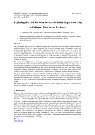
Vol.2, No.11&12, 2011

Table 8: Estimated Model Based on Equation (4) - Dependent Variable: DLog (POP) t

Variable Coefficient t-statistics Probability

Log(POP) t −1 -1.232 -11.925* 0.0000

Log(HCR) t −1 0.027 0.815 0.4228

Log(CO2) t −1 -0.400 -8.515* 0.0000

POPDUM t 0.036 -2.070** 0.0493

β0 0.779 6.632* 0.0000

Dlog(POP) t −1 0.427 4.079* 0.0004

Dlog(HCR) t −1 0.005 0.135 0.893

Dlog(CO2) t −1 0.307 2.679** 0.0131

MA (2) 1.319 5.661* 0.0000

11. Model criteria / Goodness of Fit:
R-square = 0.629; Adjusted R-square = 0.505; Wald F-statistic = 47.935 [0.0000]*
111. Diagnostic Checking:
ARCH (1) = 2.690 [0.111]; RESET = 1.057 [0.359] WHITE Test = 1.132 [0.392];
JB = 0.637 [0.726]; LM (2) = 1.543 [0.234]

Table 9. Long-Run elasticities and Short-run elasticities of Population in Pakistan
Based on Equation (4)
Variable Coefficient
HCR 0.022
CO2 -0.324*
POPDUM 0.029**

1. Long-run Estimated Coefficient
∆HCR ∆CO 2
11. Short-run Causality Test (Wald Test F-statistic): 0.018 7.180 *
* denote significant at 1% level. Figures in brackets refer to marginal significance values.
Sources: Calculated by the Authors
(0.893) (0.010)

Figure 1: Poverty Statistics at Rural, Urban and National Level (1979-2006)

47 | P a g e
www.iiste.org

45
%
40

Journal of Economics and Sustainable Development
35 www.iiste.org
30
Vol.2, No.11&12, 2011
25 RPOV
UPOV
20 NPOV

15

10

5

0
1979 1985 1986 1987 1988 1991 1993 1994 1997 1999 2002 2005 2006
Years

Note: RPOV, UPOV and NPOV represent rural, urban and national poverty

Figure 2: Data Trend for Poverty, Population and Carbon Dioxide Emissions (1975-2009)

48 | P a g e
www.iiste.org

Vol.2, No.11&12, 2011

CO2 HCR
1.0 45

0.9
40
0.8
35
0.7
30
0.6

0.5 25

0.4 20

0.3 15
5 10 15 20 25 30 35 5 10 15 20 25 30 35

POP
3.2

3.0

2.8

2.6

2.4

2.2

2.0
5 10 15 20 25 30 35

Source: World Bank (2009) and GoP (2010).

Figure 3: Conceptual Framework

Poverty Pollution Population
(HCR) (CO2) (POP)

Source: Self Extract

49 | P a g e
www.iiste.org

Vol.2, No.11&12, 2011

Figure 4: Data trends at their First Difference

D(CO2)
.08
D(HCR)
8
.06
6
.04
4
.02
2
.00
0
-.02
-2
-.04
5 10 15 20 25 30 35 -4
5 10 15 20 25 30 35

D(POP)
.05

.00

-.05

-.10

-.15

-.20

-.25

-.30
5 10 15 20 25 30 35

Source: World Bank (2009) and GoP (2010).

50 | P a g e
www.iiste.org

International Journals Call for Paper
The IISTE, a U.S. publisher, is currently hosting the academic journals listed below. The peer review process of the following journals
usually takes LESS THAN 14 business days and IISTE usually publishes a qualified article within 30 days. Authors should
send their full paper to the following email address. More information can be found in the IISTE website : www.iiste.org

Business, Economics, Finance and Management PAPER SUBMISSION EMAIL
European Journal of Business and Management EJBM@iiste.org
Research Journal of Finance and Accounting RJFA@iiste.org
Journal of Economics and Sustainable Development JESD@iiste.org
Information and Knowledge Management IKM@iiste.org
Developing Country Studies DCS@iiste.org
Industrial Engineering Letters IEL@iiste.org

Physical Sciences, Mathematics and Chemistry PAPER SUBMISSION EMAIL
Journal of Natural Sciences Research JNSR@iiste.org
Chemistry and Materials Research CMR@iiste.org
Mathematical Theory and Modeling MTM@iiste.org
Advances in Physics Theories and Applications APTA@iiste.org
Chemical and Process Engineering Research CPER@iiste.org

Engineering, Technology and Systems PAPER SUBMISSION EMAIL
Computer Engineering and Intelligent Systems CEIS@iiste.org
Innovative Systems Design and Engineering ISDE@iiste.org
Journal of Energy Technologies and Policy JETP@iiste.org
Information and Knowledge Management IKM@iiste.org
Control Theory and Informatics CTI@iiste.org
Journal of Information Engineering and Applications JIEA@iiste.org
Industrial Engineering Letters IEL@iiste.org
Network and Complex Systems NCS@iiste.org

Environment, Civil, Materials Sciences PAPER SUBMISSION EMAIL
Journal of Environment and Earth Science JEES@iiste.org
Civil and Environmental Research CER@iiste.org
Civil and Environmental Research CER@iiste.org

Life Science, Food and Medical Sciences PAPER SUBMISSION EMAIL
Journal of Biology, Agriculture and Healthcare JBAH@iiste.org
Food Science and Quality Management FSQM@iiste.org
Chemistry and Materials Research CMR@iiste.org

Education, and other Social Sciences PAPER SUBMISSION EMAIL
Journal of Education and Practice JEP@iiste.org
Journal of Law, Policy and Globalization JLPG@iiste.org Global knowledge sharing:
New Media and Mass Communication NMMC@iiste.org EBSCO, Index Copernicus, Ulrich's
Journal of Energy Technologies and Policy JETP@iiste.org Periodicals Directory, JournalTOCS, PKP
Historical Research Letter HRL@iiste.org Open Archives Harvester, Bielefeld
Academic Search Engine, Elektronische
Public Policy and Administration Research PPAR@iiste.org Zeitschriftenbibliothek EZB, Open J-Gate,
International Affairs and Global Strategy IAGS@iiste.org OCLC WorldCat, Universe Digtial Library ,
Research on Humanities and Social Sciences RHSS@iiste.org NewJour, Google Scholar.

Developing Country Studies DCS@iiste.org IISTE is member of CrossRef. All journals
Arts and Design Studies ADS@iiste.org have high IC Impact Factor Values (ICV).

11.exploring the link between poverty pollution-population (0003www.iiste.org call for-paper_ps)

Recomendados

Recomendados

Más contenido relacionado

La actualidad más candente

La actualidad más candente (20)

Similar a 11.exploring the link between poverty pollution-population (0003www.iiste.org call for-paper_ps)

Similar a 11.exploring the link between poverty pollution-population (0003www.iiste.org call for-paper_ps) (20)

Más de Alexander Decker

Más de Alexander Decker (20)

Último

Último (20)

11.exploring the link between poverty pollution-population (0003www.iiste.org call for-paper_ps)