Fractal characterization of dynamic systems sectional images

Journal of Information Engineering and Applications www.iiste.org
ISSN 2224-5782 (print) ISSN 2225-0506 (online)
Vol 2, No.7, 2012

Fractal Characterization of Dynamic Systems Sectional
Images

Salau T.A.O.1 Ajide O.O.*2
Department of Mechanical Engineering, University of Ibadan, Nigeria
* E-mail of the corresponding author: ooe.ajide@mail.ui.edu.ng

Abstract
Image characterizations play vital roles in several disciplines of human endeavour and engineering
education applications in particular. It can provide pre-failure warning for engineering systems; predict
complex diffusion or seeping of radioactive substances and early detection of defective human body
tissues among others. It is therefore the object of this study to simulate three selected known surfaces
that are of engineering interest, pass section plane through these surfaces arbitrarily and use fractal disk
dimension to characterize the resulting image on the sectioned plane. Three carefully selected surfaces
based on their engineering education and application worth’s were simulated with respective relevant
set of equations. In each case studied, the simulation was driven either by random number generation
with seed value of 9876 coupled with relevant set of equations or by numerical integration based on
Runge-Kutta fourth order algorithms or combination of both. However, all simulations were coded in
FORTRAN 90 Language. Section plane was passed through each simulated surface arbitrarily and in
two hundred (200) different times for the purpose of obtaining reliable results only. Image obtained at
less or equal to four percent (4%) tolerance level by sectioning was characterised by optimum disks
counting algorithms implemented over ten (10) scales of observations and five (5) different iteration
each. The estimated disk dimension was obtained by implementing the least square regression
procedures on optimum disks counted at corresponding scales of observations. A visual and fractal disk
dimension characterization of selected images on sectioned plane form cases studied validated
algorithms coded in FORTRAN 90 computer language. The surface of Case-III is the most rough with
disk dimension of 2.032 and 1.6% relative error above the dimension of smooth surface (2.0). This is
followed by Case-II with disk dimension of 1.905 and 4.8% relative error below the dimension of
smooth surface. Case-I has the least disk dimension of 1.897 and with 5.2% relative error below
smooth surface. Case-I and case-II that suffered negative relative error originated from set of linear
systems while Case-III that suffered positive relative error originated from set of non linear systems.
Non linearity manifested in graphical display of disk distribution by frequency in Case-III by multiple
peaks and substantial shift above disk dimension of 1.0.This study has demonstrated the high
potentiality of fractal disk dimension as characterising tool for images. The coded algorithms can serve
well as instruction material for students of linear and non linear dynamic systems.
Keywords: Fractal, Sectional Images, Fractal Disk Dimension, Dynamic Systems and Algorithms

1. Introduction
Fractal has become an important subject tool in all spheres of disciplines for characterization of
different images of objects. According to Oldřich et al (2001), Fractals can be described as rough or
fragmented geometric shape that can be subdivided in parts, each of which is (at least approximately) a
reduced copy of the whole. They are crinkly objects that defy conventional measures, such as length
and are most often characterized by their fractal dimension. They are mathematical sets with a high
degree of geometrical complexity that can model many natural phenomena. Almost all natural objects
can be observed as fractals (coastlines, trees, mountains, and clouds).Their fractal dimension strictly
exceeds topological dimension. Michael thesis in 2001 developed a structure suitable to study the
roughness perception of natural rough Surfaces rendered on a haptic display system using fractals. He
employed fractals to characterize one and two dimensional surface profiles using two parameters, the
amplitude coefficient and the fractal dimension. Synthesized fractal profiles were compared to the
profiles of actual surfaces. The Fourier Sampling theorem was applied to solve the fractal amplitude
characterization problem for varying sensor resolutions. Synthesized fractal profiles were used to
conduct a surface roughness perception experiment using a haptic replay device. Findings from the
research revealed that most important factor affecting the perceived roughness of the fractal surfaces is

21

Vol 2, No.7, 2012

the RMS amplitude of the surface. He concluded that when comparing surfaces of fractal dimension
1.2-1.35, it was found that the fractal dimension was negatively correlated with perceived roughness.
Alabi et al (2007) explored a fractal analysis in order to characterize the surface finish quality of
machined work pieces. The results of the study showed an improvement in the characterization of
machine surfaces using fractal. The corrosion of aluminium foils in a two-dimensional cell has been
investigated experimentally (Terje et al, 1994). The corrosion was allowed to attack from only one side
of an otherwise encapsulated metal foil. A 1M NaCl (pH=12) electrolyte was used and the experiments
were controlled potentiostatically. The corrosion fronts were analyzed using four different methods,
which showed that the fronts can be described in terms of self-affine fractal geometry over a significant
range of length scales. It has been demonstrated that a certain amount of order can be extracted from an
apparently random distribution of pores in sedimentary rocks by exploiting the scaling characteristics
of the geometry of the porespace with the help of fractal statistics (Muller and McCauley ,1992).A
simple fractal model of a sedimentary rock was built and tested against both the Archie law for
conductivity and the Carman-Kozeny equation for permeability. The study explored multifractal
scaling of pore-volume as a tool for rock characterization by computing its experimental ( )
spectrum. The surface characteristics of Indium Tin Oxide (ITO) have been investigated by means of
an AFM (atomic force microscopy, AFM) method. The results of Davood et al in 2007 demonstrated
that the film annealed at higher annealing temperature (300°C) has higher surface roughness, which is
due to the aggregation of the native grains into larger clusters upon annealing. The fractal analysis
revealed that the value of fractal dimension Df falls within the range 2.16–2.20 depending upon the
annealing temperatures and is calculated by the height–height correlation function. Salau and Ajide
(2012) paper utilised fractal disk dimension characterization to investigate the time evolution of the
Poincare sections of a harmonically excited Duffing oscillator. Multiple trajectories of the Duffing
oscillator were solved simultaneously using Runge-Kutta constant step algorithms from set of
randomly selected very close initial conditions for three different cases. The study was able to establish
the sensitivity of Duffing to initial conditions when driven by different combination of damping
coefficient, excitation amplitude and frequency. The study concluded that fractal disk dimension
showed a faster, accurate and reliable alternative computational method for generating Poincare
sections. Some complex microstructures defy description in terms of Euclidean principles (Shu-Zu and
Angus, 1996). Fractal geometry can make numerical statements about any shape or collection of
shapes, however irregular and chaotic they may seem. In their paper, fractal analysis was applied to the
characterization of metallographic images. Kingsley et al (2004) paper presented the application of
fractal analysis for analyzing various harmonic current waveforms generated by typical nonlinear loads
such as personal computer, fluorescent lights and uninterruptible power supply. The fractal technique
make available both time and spectral information of the nonlinear load harmonic patterns. The
analysis results showed that the various harmonic current waveforms can be easily identified from the
characteristics of the fractal features. The study was able to demonstrate that the fractal technique is a
useful tool for identifying harmonic current waveforms and forms a basis towards the development of
the harmonic load recognition system.
The importance of image characterizations in science and engineering applications cannot be
overemphasized. Despite this, research efforts have not been significantly explored to characterize
dynamic systems sectional images using fractal. This paper is intends to partly address this gap by
specifically characterising the sectional images/surfaces of tools or systems such as Hollow sphere,
Transmissibility ratio and Lorenz weather model using fractal disk dimension.

2. Theory and Methodology
Three systems were selected for reasons of linearity, nonlinearity, familiarity and relative degree of
roughness of surface. These systems are hollow sphere and transmissibility ratio belonging to linear
system and are well known to have smooth surfaces. The third system is Lorenz weather equations
belonging to nonlinear system and the surface is known to be rough due to chaotic behaviour of the
system. The governing equations for the three (3) systems are listed in equations (1) to (9).

2.1 Hollow Sphere (Case-I):

X = Radius * Sin(ϕ1 )* Cos(ϕ2 ) (1)

Y = Radius * Sin(ϕ1 )* Sin(ϕ2 ) (2)

22

Vol 2, No.7, 2012

Z = Radius * Cos(ϕ1 ) (3)

In equations (1) to (3), X=Cartessian coordinate of arbitray point on the sphere in x-direction, Y=
Cartessian coordinate of arbitray point on the sphere in y-direction and Z= Cartessian coordinate of

arbitray point on the sphere in z-direction. Similarly ϕ1 and ϕ2 =Angle measured in radian. In

addition 0 ≤ ϕ1 ≤ π and 0 ≤ ϕ2 ≤ 2π . A good representative number of points on the sphere and

fairly uniformly distributed can be obtained by iterative reseting of ϕ1 and ϕ 2 randomly and for
fixed radius in equations (1) to (3).

2.2 Transmissibility Ratio (Case-II):
This is a dynamic terminology for expressing the technology art of reducing drastically the amount of
force transmitted to the foundation due to the vibration of machinery using springs and dampers. The
transmissibility ratio is given by equation (4).

1 + 4ao 2γ 2
TR = (4)
(1 − ao 2 ) 2 + 4ao 2γ 2

In equation (4) TR = ratio of the transmitted force to the impressed force, ao =frequency ratio and γ

= damping factor. By letting X ← ao , Y ← γ and Z ← TR , a transmissibility ratio surface can

be created within the specified lower and upper limits of ao and γ respectively. A good
representative number of points on the transmissibility ratio surface and fairly uniformly distributed

can be obtained by iterative resetting of ao and γ randomly within their specified limits and

evaluation of the corresponding transmissibility ratio by equation (4).

2.3 Lorenz Weather Model (Case-III):
This is a mathematical model for thermally induced fluid convection in the atmosphere proposed by
Lorenz in 1993 (see Francis (1987).
•
X = σ (Y − X ) (5)

•
Y = ρ X − Y − XZ (6)

•
Z = XY − β Z (7)
The steady solutions of the rate equations (5) to (7) can be sought numerically and simultaneously.
Similarly, the steady values of X, Y, and Z variables can be used to represent an arbitrary points on the
‘Lonrenz surface’ in x, y and z-Cartesian directions respectively. In equations (5) to (7) we have X =
Amplitude of fluid velocity related variable while Y and Z measures the distribution of temperature.
The parameters σ and ρ are related to the Prandtl number and Rayleigh number, respectively, and
the third parameter β is a geometric factor. A good representative number of points on the ‘Lonrenz
surface’ can be obtained by setting fixed value for the parameters, σ , ρ and β and then use

23

Vol 2, No.7, 2012

Runge-Kutta fourth order algorithm to iteratively and simultaneously solve the rate equations (5) to (7)
using constant time step.

2.4 Plane Equation:
Each of the three systems selected were simulated using their respective equations and were similarly
sectioned several time with arbitrarily chosen cut plane. The corresponding sectional results were
characterised with fractal disk dimension based on optimum disks counted algorithm coded in
FORTRAN-90 Language. The general equation of an arbitary plane is given by equation (8).

C1 X + C2Y + C3 Z + C4 = 0 (8)

In equation (8), C1 to C4 are constants coefficient. Similarly X, Y, and Z are arbitrary coordinates
on the plane. Thus the constants can be solved for three set of (X, Y, Z) taken randomly on the arbitrary
plane.
The distance (D) between a reference point (Q) and an arbitrary point (P) on an arbitrary plane is given
by equation (9).
uuu
r
PQ. n
D= (9)
n
uuu
r
In equation (9) PQ is a vector quantity and n is a vector normal to the arbitary plane. Similarly n
is the absolute length of normal vector (n).

2.5 Fractal Disk Dimension:
The three cases refers, sectioned was performed large number of time at tolerance level of less or equal
to four percent (4%) for convenience reason only. The resulting images on the sectioned plane was
further analysed for their corresponding dimension using optimum disks counting algorithms
implemented in 3-dimensional Euclidean space. The disks counting was performed iteratively five time
(5) each and over ten (10) different scales of observations that are related to the characteristic length of
the image on the sectioned plane. Characteristic length is defined as the longest absolute distance
between pair points of the image on the sectioned plane. The disk dimension of images obtained on
sectioned plane were estimated by performing least square regression analysis on scales of observation
and the corresponding minimum disks counted for full covering of the image. The scales of
observations and corresponding minimum disks counted are expected to relate according to power law
given by equation (10).

Ydisks ∝ Scale Ds (10)

In proportional equation (10), Ydisks =minimum number of disks required for the full cover of the

image on the sectioned plane at specified observation scale while Ds =disk dimension of the image. By

introducing equality constant (K) in proportional equation (10) and taking the logarithm of the right

and left sides of the resulting equation, a linear equation (11) emerged as function of Ydisks , K,

Scale and Ds .

YL = Ds X L + C (11)

24

Vol 2, No.7, 2012

In equation (11), YL , X L and C are logarithm of Ydisks , Scale and K respectively. The disk
dimension of the image on the sectioned plane is therefore the slope of the line of best fit to collection

of YL and X L .

The dimension of the surface studied ( Dsurface ) was validated by equations (12) and (13) noting that

Dave =average disk dimension of collection of dimension of images on large number of arbitrary
sectioned planes (N).

Dsurface = 1.0 + Dave (12)

i=N
1
Dave =
N
∑ (D )
i =1
s i (13)

2.6 Input Parameters Setting for Studied Cases:
Common to all studied cases are large number of arbitrary sectioned plane (N) set at 200, disk
dimension distribution by frequency of 20 units subinterval between lower and upper limits and ten
(10) scales of observation for five (5) independent iterations each.
Case-I:
Radius of sphere used was 10 units. Number of points on the sphere generated randomly before
sectioning commence was 9000 with generating seed value of 9876. Tolerance was set at less or equal
four percent (4%).
Case-II:

Frequency ratio 0 ≤ ao ≤ 10 and damping factor 0.1 ≤ γ ≤ 1.0 was selected random with
generating seed value of 9876. The number of points on the transmissibility ratio surface generated
randomly before sectioning commence was 9000 only. Tolerance was set at less or equal four percent
(4%).
Case-III:
8
Initial conditions (X, Y, Z) was set at (1, 0, 1) for σ =10, ρ =28, and β = = 2.6667 . The
3
integration was performed with constant time step ( ∆t = 0.01 ). The number of points on the ‘Lorenz
surface’ generated was 9000 after 1000 unsteady solutions points was discarded for sectioning purpose.
The random numbers required was generated with seed value of 9876. Tolerance was set at less or
equal four percent (4%).
Three systems were selected for reasons of linearity, nonlinearity, familiarity and relative degree of
roughness of surface. These systems are hollow sphere and transmissibility ratio belonging to linear
system and are well known to have smooth surfaces. The third system is Lorenz weather equations
belonging to nonlinear system and the surface is known to be rough due to chaotic behaviour of the
system. The governing equations for the three (3) systems are listed in equations (1) to (9).

25

Vol 2, No.7, 2012

3. Results and Discussion
A sample sectioned results for Case-I, Case-II and Case-III are shown in figures 1 to 3 respectively.

XY-Projection YZ-Projection

8.0
15.0

6.0
10.0
4.0

2.0
5.0
0.0
-8.0 -6.0 -4.0 -2.0 0.0 2.0 4.0 6.0

Z-Value
Y-Value

-2.0
0.0
-12.0 -10.0 -8.0 -6.0 -4.0 -2.0 0.0 2.0 4.0 6.0 8.0
-4.0

-6.0 -5.0

-8.0

-10.0
-10.0

-12.0
X-Value -15.0
Y-Value

Figure 1 (a) Figure 1 (b)

XZ-Projection

15.0

10.0

5.0
Z-Value

0.0
-10.0 -5.0 0.0 5.0
-5.0

-10.0

-15.0
X-Value

Figure 1 (c)

Figure 1: A section through a Hollow Sphere with Plane equation:

182.96 X + 124.96Y + 16.23Z + 439.92 = 0.00

This plane is located at -439.92 unit perpendicular distance from the origin.Referring to figure 1, the
images observed on the projected sectioned plane agreed perfectly with dot or circular or ellipse
expected for section through a hollow sphere. Thus the simulation algorithms codes in FORTRAN-90
can be adjudged working perfectly.

26

Vol 2, No.7, 2012


1.20 1.20

1.00 1.00

0.80 0.80

Z-Value
Y-Value

0.60 0.60

0.40 0.40

0.20 0.20
0.00
0.00
0.00 0.50 1.00 1.50
0.00 5.00 10.00 15.00
Y-Value
X-Value


XZ-Projection

1.20

1.00

0.80
Z-Value

0.60

0.40

0.20

0.00
0.00 5.00 10.00 15.00

X-Value

Figure 2 (c)

Figure 2: A section through Transmissibility Ratio Surface with Plane equation:

−0.10 X + 2.10Y − 2.05 Z − 0.03 = 0.00

This plane is located at 0.03 unit perpendicular distance from the origin.

27

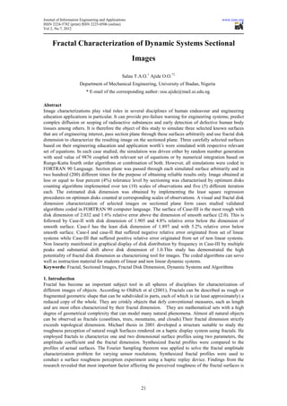
Vol 2, No.7, 2012


30 50
25 45
20 40
15 35

Z-Value
30
Y-Value

10
25
5 20
0 15
-20 -10 -5 0 10 20 10
-10 5
-15 0
-20 -20 0 20 40
X-Value Y-Value


XZ-Projection
60

40
Y-Value

20

0
-20 -15 -10 -5 0 5 10 15 20
X-Value

Figure 3 (c)

Figure 3: A section through ‘Lorenz Surface’ with Plane equation:

−0.10 X + 0.01Y − 0.01Z + 0.012 = 0.00

This plane is located at -0.012unit perpendicular distance from the origin.

Figures 1 to 3 shows sample of the variability of structure of the surfaces studied. The disk dimension
estimated for the structured solution points on the sectioned planes were 0.890, 0.605 and 1.077 for
Case-I, Case-II and case-III respectively. Thus the structured solution points from Lorenz system is the
most rough, followed by hollow sphere and transmissibility ratio respectively. These observation
matches perfectly with visual assessment of the images.

28

Vol 2, No.7, 2012

Table 1: Disk Dimension Distribution Based on Natural Distribution of Solution Points on 200
Arbitrarily Selected Sectioned Planes
S/N Case-I Case-II Case-III
AD FQ AQ AD FQ AQ AD FQ AQ
1 0.129 0.005 0.001 0.035 0.002 0.000 0.245 0.005 0.001
2 0.207 0.000 0.000 0.104 0.000 0.000 0.303 0.000 0.000
3 0.285 0.005 0.001 0.173 0.000 0.000 0.361 0.000 0.000
4 0.363 0.010 0.004 0.242 0.000 0.000 0.418 0.000 0.000
5 0.441 0.005 0.002 0.311 0.000 0.000 0.476 0.010 0.005
6 0.519 0.015 0.008 0.381 0.000 0.000 0.533 0.005 0.003
7 0.596 0.050 0.030 0.450 0.000 0.000 0.591 0.010 0.006
8 0.674 0.065 0.044 0.519 0.008 0.004 0.649 0.005 0.003
9 0.752 0.075 0.056 0.588 0.018 0.011 0.706 0.010 0.007
10 0.830 0.120 0.100 0.657 0.044 0.029 0.764 0.010 0.008
11 0.908 0.240 0.218 0.726 0.060 0.044 0.821 0.065 0.053
12 0.986 0.250 0.247 0.796 0.094 0.075 0.879 0.045 0.040
13 1.064 0.075 0.080 0.865 0.268 0.232 0.937 0.115 0.108
14 1.142 0.015 0.017 0.934 0.212 0.198 0.994 0.180 0.179
15 1.220 0.015 0.018 1.003 0.130 0.130 1.052 0.160 0.168
16 1.298 0.015 0.019 1.072 0.116 0.124 1.110 0.135 0.150
17 1.376 0.005 0.007 1.142 0.022 0.025 1.167 0.050 0.058
18 1.454 0.015 0.022 1.211 0.010 0.012 1.225 0.050 0.061
19 1.532 0.005 0.008 1.280 0.010 0.013 1.282 0.095 0.122
20 1.610 0.010 0.016 1.349 0.006 0.008 1.340 0.045 0.060
Dave 0.897 0.905 1.032
Dsurface 1.897 1.905 2.032
Error relative to
smooth surface
(2.0) -5.2% -4.8% 1.6
Note: AD=Estimated disk dimension, FQ=Frequency and AQ=product of AD & FQ.

Referring to table 1, ‘Lorenz surface’ is the most rough with disk dimension of 2.032 and 1.6% relative
error above the dimension of smooth surface (2.0). This is followed by Transmissibility ratio surface
with disk dimension of 1.905 and 4.8% relative error below the dimension of smooth surface. The
surface of a hollow sphere has the least disk dimension of 1.897 and with 5.2% relative error below
smooth surface. The hollow sphere surface and transmissibility ratio surface that suffered negative
relative error originated from set of linear systems while ‘Lorenz surface’ that suffered positive relative
error originated from set of non linear systems. Thus it can be argued that disk dimension measure is
very sensitive to system degree of nonlinearity.

29

Vol 2, No.7, 2012

Disk Dimension Distribution in Case-I
0.28
0.26
0.24
0.22
0.20
0.18

Frequency
0.16
0.14
0.12
0.10
0.08
0.06
0.04
0.02
0.00
0.0 0.5 1.0 1.5 2.0
Dimension

Figure 4: Disk Dimension Distribution Predicted for Case-I

Disk Dimension Distribution in case-II
0.30
0.28
0.26
0.24
0.22
Frequency

0.20
0.18
0.16
0.14
0.12
0.10
0.08
0.06
0.04
0.02
0.00
0.0 0.5 1.0 1.5
Dimension

Figure 5: Disk Dimension Distribution Predicted for Case-II

Disk Dimension Distribution in case-III
0.19
0.18
0.17
0.16
0.15
0.14
0.13
0.12
Frequency

0.11
0.10
0.09
0.08
0.07
0.06
0.05
0.04
0.03
0.02
0.01
0.00
0.0 0.5 1.0 1.5
Dimension

Figure 6: Disk Dimension Distribution Predicted for Case-III

Figures 4, 5 and 6 presents the same information contained in table 1 graphically. Figure 6 can be
differentiated by multiple peaks and substantial shift above disk dimension of 1.0. This again is a clear
manifestation of the non linear origin of the system it is associated.
4. Conclusions
This study has demonstrated successfully the integration of concept of randomness, numerical
integration with Runge-Kutta fourth order algorithms using constant time step, vectors analysis and
fractal characterization in relation to systems that are of particular interests in engineering education
and application. Bearing in mind possible computation errors, the relative roughness of one third of the
studied surfaces was validated with an estimated disk dimension of 2.032 which is 1.6% greater than
dimension (2.0) for smooth surface. In addition two third of the studied surfaces were adjudged smooth
with estimated disk dimension of 1.897 and 1.905 that are lesser than dimension (2.0) of smooth
surface by 5.2 % and 4.8% respectively. The disk dimension characterised the degree of non linearity
inherent in the studied cases.

30

Vol 2, No.7, 2012

References

(1) Alabi B., Salau T.A.O. and Oke S.A. (2007), Surface Finish Quality Characterization
of Machined Work Pieces Using Fractal Analysis. MECHANIKA, Nr.2(64), Pg. 65-71,
ISSN 1392-1207.
(2) Davood R., Ahmad K., Hamid R. F. and Amir S. H. R. (2007), Surface Characterization
and Microstructure of ITO Thin Films at Different Annealing Temperatures. Elsevier:
Applied Surface Science, Vol.253, Pg.9085-9090, Science
Direct.www.elsevier.com/locate/apsusc
(3) Francis C. Moon (1987), Chaotic Vibrations an Introduction for applied Scientists and
Engineers, John Wiley & Sons, New York, pp. 30-32, ISBN: 0-471-85685-1.
(4) Kingsley C. U., Azah M., Aini H. and Ramizi M. (2004) ,The Use of Fractal Analysis for
Characterizing Nonlinear Load Harmonics. Iranian Journal Of Electrical And Computer
Engineering, Vol. 3, No. 2
(5) Michael A.C. (2001), Fractal Description Of Rough Surfaces For Haptic Display. A Ph.D
Dissertation in Department of Mechanical Engineering, Stanford University.
(6) Oldřich Z.,Michal V., Martin N. and Miroslav B.(2001),Fractal Analysis of Image
Structures.Harfa-Harmonic and Fractal Image
Analysis,Pg.3–5.http://www.fch.vutbr.cz/lectures/imagessci/harfa.htm
(7) Roland E. Larson, Robert P. Hostetler and Bruce H. Edwards (1998), Calculus, Sixth
Edition, Houghton Mifflin Company, U.S.A. pp.737-744,761, ISBN: 0-395-86974-9.
(8) Salau T.A.O. and Ajide O.O. (2012), Fractal Characterization of Evolving Trajectories of

Duffing Oscillator, International Journal of Advances in Engineering and Technology

Research (IJAET), Vol. 2, Issue 1, Pg. 62-72.
(9) Shu-Zu L. and Angus H. (1996), Fractal Analysis to Describe Irregular Microstructures.
Journal of the Minerals, Metals and Materials Society.Vol.47, No.12, Pg.14-17.
(10) Terje H.,Torsein J., Paul M. and Jens F. (1994),Fractal Characterization of
Two-Dimensional Aluninium Corrosion Fronts.APS Journals, Physical Review
E50,Pg.754-759. © 1994 The American Physical Society.
(11) William W. Seto (1983), Schaum’s Outline Series: Theory and Problems of Mechanical
Vibrations, McGraw-Hill International Book Company, Singapore, pp. 5, ISBN:
0-07-099065-4.

31

This academic article was published by The International Institute for Science,
Technology and Education (IISTE). The IISTE is a pioneer in the Open Access
Publishing service based in the U.S. and Europe. The aim of the institute is
Accelerating Global Knowledge Sharing.

More information about the publisher can be found in the IISTE’s homepage:
http://www.iiste.org

The IISTE is currently hosting more than 30 peer-reviewed academic journals and
collaborating with academic institutions around the world. Prospective authors of
IISTE journals can find the submission instruction on the following page:
http://www.iiste.org/Journals/

The IISTE editorial team promises to the review and publish all the qualified
submissions in a fast manner. All the journals articles are available online to the
readers all over the world without financial, legal, or technical barriers other than
those inseparable from gaining access to the internet itself. Printed version of the
journals is also available upon request of readers and authors.

IISTE Knowledge Sharing Partners

EBSCO, Index Copernicus, Ulrich's Periodicals Directory, JournalTOCS, PKP Open
Archives Harvester, Bielefeld Academic Search Engine, Elektronische
Zeitschriftenbibliothek EZB, Open J-Gate, OCLC WorldCat, Universe Digtial
Library , NewJour, Google Scholar

Fractal characterization of dynamic systems sectional images

Recomendados

Recomendados

Más contenido relacionado

La actualidad más candente

La actualidad más candente (19)

Destacado

Destacado (7)

Similar a Fractal characterization of dynamic systems sectional images

Similar a Fractal characterization of dynamic systems sectional images (20)

Más de Alexander Decker

Más de Alexander Decker (20)

Último

Último (20)

Fractal characterization of dynamic systems sectional images