Tax policy, inflation and unemployment in nigeria (1970 – 2008)

European Journal of Business and Management www.iiste.org
ISSN 2222-1905 (Paper) ISSN 2222-2839 (Online)
Vol.5, No.15, 2013
114
Tax Policy, Inflation and Unemployment in Nigeria (1970 – 2008)
Johnson A. Atan, PhD
Department of Economics, University of Uyo, P.M.B. 1017, Uyo, Nigeria
Tel: +234 806 602 4940, E-mail: johnsonatan@yahoo.com
Abstract
This study is concerned with the use of tax policy in the management of a real-world economy, the Nigerian
Economy. It examines the attempts by successive Nigerian governments to use taxation to influence
macroeconomic aggregates, especially inflation and unemployment, and covers the period 1970 to 2008. It is
largely a secondary data study, focussing on the extent to which these variables responded to changes in
government’s tax measures. Data on these variables for the thirty-nine year period were analysed using both
descriptive and inferential statistical techniques. The Ordinary Least Square (OLS) method was used for the
estimations. The analysis shows that the historical trends in inflation and unemployment showed no significant
response to tax policy between the period 1970 and 2008. Periods of lower taxes recorded lower inflation rate in
some years and higher inflation rates in some years. Unemployment rates increased steadily in some years
whether taxes were raised or lowered. Government in some years lowered taxes amidst high inflation rates in the
economy. Taxes have a negative effect on the inflation rate in line with the theory, but with insignificant
coefficient. In the case of unemployment rate, the regression results show a negative relationship between tax
policy and unemployment, but with insignificant coefficient, which is contrary to the theory. The analysis shows
that tax policy was not effective in controlling inflation, and tackling unemployment problems in the economy
during the period of study largely because of inconsistency in the use of tax measures. It is recommended that
government apply tax measures much more carefully than was observed over the period studied.
Keywords: Tax Policy, Inflation, Unemployment, Economic Management and Nigeria.
1. Introduction
Economic theory presents taxation as a major tool of macroeconomic management. The idea is that taxation,
usually in combination with some other policy tools, can be used to steer the economy in the direction that is
desired. It is argued that if, for instance, the economy is experiencing a depression, the government could use tax
policy to stimulate the system and cause a recovery. If, on the other hand, the economy is experiencing
inflationary pressures, tax policy could be used to reduce the pressures and stabilize the system. These arguments
make taxation a particularly important management tool of economic management.
In Nigeria, taxation has been a major component of the policy measures of successive governments since
independence in 1960. Between 1961 and 2008, several amendments – more than 29 tax acts – were enacted.
Such actions, which form the basis of the government’s fiscal policy are formulated to either “gear up” or
stabilize the economy (Ukpong and Akpakpan, 1998).
In designing and implementing the tax policies mentioned above, successive Nigerian governments expected to
achieve economic stabilization as promised by economic theory. In particular, they expected to achieve sustained
low levels of unemployment and inflation over the years. But, as records show, the objectives of the
governments were not achieved. Instead of stability, the Nigerian economy exhibited instability in the major
economic aggregates – unemployment and price level (inflation). For instance, in the 2003 and 2004 annual
budgets, the projected inflation rate was 9 percent, but the actual inflation rate stood at 10.01 percent by
December 2003 and 11.57 percent in 2004 (CBN, Annual Report, 2004). A similar situation was observed with
respect to unemployment rate, and the state of affairs in the last years of the period being studied - 2007 and
2008, were not different.
For a period of about 30years, tax policy failed to steer the Nigerian economy in the direction that was desired by
policymakers. From 1971 to 1974, a six months’ ban was enforced on some selected items. Between 1975 and
1977, some import duty rates were raised while others were lowered. In 1980, there was a reduction rates from
10 – 25% to 5 – 15% to liberalize imports for certain specific commodities. In 1986 and 1987, adjustments were
made in customs and excise tariff. These were to reduce the inflationary pressure consequent upon increased
aggregate demand on the economy. Between 1987 and 1996, the terminal rate of personal income tax was
reduced from 70% to 55% to encourage consumption and stimulate output leading to reductions in
unemployment. Similarly, company tax rate was reduced from 45% in 1986 to 30% with effect from 1996.
Value-added-tax (VAT) was introduced in 1994 at a flat rate of 5% to replace a variety of sales taxes that were
imposed at state level. From 2000 to 2008, government desired to broaden the tax base, lower the tax rates on
personal and corporate incomes, and reduce the tariffs on major raw materials inputs for a number of imported
finished products. These were aimed at encouraging production through increased investment and consumption
spending and the redressing of external disequilibrium.

Vol.5, No.15, 2013
115
In addition to changes in tax rates reviewed above, a review of some immediate past budget speeches of the
Nigerian government reveal that the intention of government was to use taxation to stimulate the economy –
using tax policy to influence purchasing power and production costs. Indeed, the broad policy objectives were to:
ensure price stability; attain job creation and employment opportunities; and achieve balance of payments
equilibrium.
As outlined in the introductory notes, the various tax measures failed to produce the expected conditions – they
failed to stabilise the economy – and stabilisation remained the major objective of succeeding governments. But
in their efforts to improve the performance of the economy, the governments have continued to stress tax policy
with no indication as to why the society should expect better outcomes this time, and economic textbooks
continue to emphasize the potency of taxation as a tool of economic management. This makes it necessary to
investigate what was done in the use of taxation in controlling inflation and unemployment rates in the Nigerian
economy during the period chosen for study. This is done in the following sections. Following the introduction,
section 2 looks at the theoretical/conceptual issues. In section 3, the inflation and unemployment models of the
Nigerian economy were specified. Section 4 presents and discusses the data and regression results, while section
5 presents the major findings and concludes the paper.
2. Theoretical/Conceptual Issues
Taxation plays an important role in economic management of nations. Economies all over the world employ tax
policy to improve their fiscal and economic performance. In the short run policy-makers formulate tax policies to
complement expenditure restraint aimed to contain macroeconomic imbalances (Bovenberg, 1985).
Governments can regulate the economy (that is, encourage or discourage particular forms of social behaviour) by
manipulating the incidence of taxation. Tax incentives, for example, tax reduction, tax holidays, are given
usually to promote investment and boost output. The reverse also applies: a heavy tax on luxury goods is likely
to reduce public demand for such items and shift productive resources to other areas (Smartrakalev, 2005).
By this brief analysis, Smartrakalev tries to explain that, taxes are at the foundation of public finances; they are
the principal means by which governments fund their expenditures. Optimal tax policy goes beyond mere
efficiency and funding considerations to encompass inevitable normative judgments about the amount of
redistribution. This implies that taxation and tax policy can be used to control and direct economic management.
The regulative role of taxation is one of the most pronounced roles from the fiscal policy proponents. “The
optimal tax policy turns out to affect the economy countercyclically via procyclical taxes, that is, ‘cooling down’
the economy with higher taxes when it is ‘overheated’ due to a positive productivity shock” (Ljungqvist & Uhlig
2000). The explanation is that agents would otherwise end up consuming too much in boom times since they are
not taking into account the “addiction effect” of a higher consumption level. In recessions, the effect goes the
other way round and taxes should be lowered to “stimulate” the economy by bolstering consumption.
According to Wasylenko (1997), at one level, that tax policy influences economic behaviour has become a basic
tenet for economic policymakers. For example, taxation is assumed to influence multinational firms’ financial
decisions about repatriation of profits. The economics of Taxation, therefore, is about how best taxes of various
forms can achieve their objectives. The purposes of taxation go beyond the raising of sufficient revenue to cover
the cost of government operations; they include the stabilization of economic activity, achievement of full
employment of resources, maintenance of a favourable balance of payments (BOPs), and promotion of economic
growth.
A country’s tax is a major determinant of other macroeconomic indexes. Specifically, for both developed and
developing economies, there exists a relationship between tax structure and the level of economic growth and
development. Indeed, it has been argued that the level of economic development has a very strong impact on a
country’s tax base and tax policy objectives vary with the stages of development (Hinricks, 1966; Musgrave,
1969) as quoted by Ariyo (1997). Similarly, the (economic) criteria by which a tax structure is to be judged and
the relative importance of each tax source vary over time (Musgrave, 1969). For example, during the Colonial
era and immediately after the Nigerian independence in 1960, the sole objective of taxation was to raise revenue.
Later on, emphasis shifted to the infant industries’ protection and income redistribution objectives.
In his discussion of the relationship between tax policy and economic development, Musgrave (1969), according
Ariyo, (1997), divided the period of economic development into two: the early period when an economy is
relatively underdeveloped and the later period when the economy is developed. The early period of economic
development is characterized by the dominance of agricultural taxation which serves as a proxy for personal
income taxation. Agricultural taxation substituted for personal income tax given the difficulty in reaching
individual farmers and the availability to measure their tax liability accurately. This problem thereby necessitates
the use of the ability-to-pay principle, effectively limiting personal income taxation to the wage income of civil
servants and employees of large firms both of which account for an insignificant proportion of the total working
population.

Vol.5, No.15, 2013
116
At this stage of economic development, direct taxes cannot be important because there are few home-based
industries. The same principle applies to excise tax (an indirect tax) on locally manufactured goods. Both will
increase in relative importance as economic development progresses due to growth or non-static nature of the
bases of these taxes. Several retail outlets also make a sales tax system difficult to implement and a multiple-
stage sales tax system even more so (Musgrave 1969). Further, the rudimentary nature of the economy precludes
retail form of taxes.
Economic development brings with it an increase in the share of direct taxes in total revenue. This is consistent
with the experience of developed economies in which direct taxes for example, personal income tax becomes
important as the share of employment in the industrial sector increases. Also, as the dominance of the
agricultural sector decreases, sales tax may be broadened because a great deal of output and income will go
through the formal market as the economy becomes more monetized.
Musgrave (1969) as cited in Ariyo (1997), noted that at this stage taxes might be imposed on firms or individuals
on expenditures or receipts, and on factor inputs or products, among others. He further argued that there would
be a tendency to shift from indirect to direct taxes. His theory relates to a normal development process. However,
to Ariyo (1997), the theory does not consider a situation where the sudden emergence of an oil-boom provides an
unanticipated source of huge revenue. Taxes in which ever form, should possess some good qualities for fairness
and equitability.
Adam Smith and other classical economists, in their canon of taxation, had documented what should constitute a
good tax. A good tax, ipso facto, should possess the following attributes:
a) The distribution of the tax burden should be equitable i.e., everybody should pay his/her fair share;
b) Taxes should be chosen so as to minimize interference with economic decisions in otherwise efficient
markets. Such interference imposes “excess burden” which should be minimized;
c) Where tax policy is used to achieve other objectives such as to grant investment incentives, this
should be done so as to minimize interference with the equity of the system;
d) Tax structure should facilitate the use of fiscal policy for stabilization and growth objectives;
e) The tax system should permit fair and non arbitrary administration and it should be understandable to
the tax payer;
f) Administration and compliance cost should be as low as is compatible with the other objectives
(Musgrave and Musgrave 1989:216).
The various objectives are not necessarily in agreement and where they conflict, tradeoffs between them are
needed. Thus, equity may require administrative complexity and may interfere with neutrality, efficient design of
tax policy may interfere with equity, and so forth.
Adawo (2001), in support of the classical attributes of taxes, maintained that a tax system should be equitable i.e.,
each tax payer should contribute his/her ‘fair share’ to the cost of government. But the term ‘fair share’ is not
easy to define. In particular, two strands of thought may be distinguished. One approach rests on the benefits
principle. According to this theory, an equitable tax system is one under which each tax payer contributes in line
with benefits, which he/she receives from public services. The benefit criterion, therefore, is not one of tax
policy only but of tax-expenditure policy. Here economics of the public sector is viewed as involving a
simultaneous solution to both its revenue and its expenditure aspects.
The other strand rests on the ability-to-pay principle. Here the tax problem is viewed by itself independent of
expenditure determination. A given revenue is needed and each tax payer is asked to contribute in line with his
or her ability to pay. This approach leaves the expenditure side of the public sector dangling and is thus less
satisfactory from the economists’ point of view (Musgrave and Musgrave, 1989:219). But actual tax policy is
largely determined independent of the expenditure and an equity rule is needed to provide guidance. The ability
to pay principle is widely accepted as a guide.
However, neither approach is easy to interpret or implement. For the benefit principle to be applied, expenditure
benefits for particular tax payers must be known. For ability-to-pay approach to be applicable, it is necessary to
know how this ability is to be measured. These are difficulties and neither approach wins on a practical ground.
Moreover, neither approach can be said to deal with the entire function of tax policy.
The benefit approach will allocate that part of the tax bill which defrays the cost of public services, but it cannot
handle taxes needed to finance transfer payments and serve re-distributional objectives.
For benefit taxation to be equitable, it must be assumed that a ‘proper’ state of distribution exists. In practice,
there is no separation between the taxes used to finance public services and the taxes used to redistribute income.
The ability-to-pay approach meets the redistribution problem but leaves the provision for public services
undetermined.
But as Musgrave and Musgrave (1989:219), have argued, both principles have important, if limited, application
in designing an equitable tax structure, one which is acceptable to most people and preferable to alternative
arrangement.

Vol.5, No.15, 2013
117
In a modern economy, taxes are not just designed to raise revenue for government, it is in addition, an instrument
of economic management, an instrument for controlling the economy. The control consists in regulating
spending to ensure that the right levels are achieved; that is, levels that enable the system to avoid recession and
inflation (Akpakpan, 1999).
To be able to manage the economy in such a way that neither a recession nor an inflation occurs, the government
must assess the economic situation. It must determine accurately whether the economy needs to be stimulated,
and to what extent; whether it needs to be restrained, and to what extent; or whether things are all right. The
assessment of the economy in this wise, determines the kind of taxes to be introduced, which will in turn
determine, to a large extent, the state of the economy. Where the government’s assessment suggests that the
economy needs to be stimulated, a lower tax rate is usually introduced to boost spending where it suggests that it
needs to be restrained, a higher tax rate is usually introduced to reduce spending.
With taxes, government can control the working of the economy in terms of encouraging or discouraging
spending, reducing inflation and unemployment rates, and maintaining a favourable balance of payments.
2.1 Tax Policy and the Control of Inflation and Unemployment
The government can use taxation to steer the economy in a desired direction (Akpakpan, 1999). If the
government wishes to stimulate the economy, it could do so by cutting taxes. A tax cut leaves more money in the
hands of people to spend. This simple policy prescription of reducing taxes will increase spending, making
production to go up and creating employment, tax revenue will also rise. If the government wishes to restrain the
economy, it could do so by increasing taxes. By so doing disposable income will fall leading to a fall in spending
and production. In this case, a tax increase will shift the consumption function down by the amount of the tax
and reduce the level of income by a multiplier effect. A tax cut, on the other hand, raises consumption and exerts
a multiplier effect on the level of income (Iniodu, 1996). During a recession (when the economy is deflationary)
government can stimulate aggregate demand by cutting taxes, which should bring about more jobs and reduce
unemployment rate and deflationary gap in the economy. If the economy is inflationary, to dampen the
inflationary pressure, the policy prescription is to contract the economy indirectly by raising taxes to discourage
consumption. Writing in these mould are Essien (2007), Iniodu (1996), McConnell and Brue (1999), Akpakpan
(1999), Anyanwu (1997), Ukpong and Akpakpan (1998), Cobham, (1981), Ekpo (2005) among others.
Strong theoretical underpinnings have been provided for tax policy as an instrument of fiscal policy in
controlling inflation and unemployment, but empirical investigation into the matter have been rather scanty.
In a study, Anyanwu (1997), investigated the effect of taxes on inflation and unemployment rates in Nigeria
between 1981 and 1996. Using data on taxes, inflation and unemployment rates during the period of study, the
results of his log-linear regression reveal a positive relationship between taxes and inflation rate, but with
insignificant coefficient. Based on this result, he concluded that taxes fuelled Nigeria’s inflation rather that
reducing it. On the unemployment rate, his findings reveal that different taxes affect Nigeria’s unemployment for
the different period between 1981-1996. He concluded that taxes vary negatively with unemployment, and with
the coefficient of unemployment being insignificant.
3. Model Specification
The analysis is done using both descriptive and inferential statistics. The descriptive statistics involved plain
description using statistical tools like averages, percentages, tables and graphs, while inferential statistics
involved the use of econometrics method of analysis.
Apart from the time series data on the individual taxes, total tax revenue and GDP, estimation of tax effects on
target variables requires a specification of the potential proxy for tax policy. For this study, we will follow
Angelopoulos, Economides and Kammas (2007), in using average tax rate (i.e. total tax revenue over GDP) as a
measure of tax policy (this is as in the literature).
3.1 The Inflation Equation
Inflation function was here specified in an equation form, using the variables identified as determinants of
inflation in Ekpo, Ndebbio, Akpakpan and Nyong (2004). It is given as:
INF = r0 + r1ATR + r2EXCHt + r3MGSt + r4OPN + r5INF-1 + e32t ..... (3.1)
Apriori expectations are:
r1 < 0, r2, r3, r4, r5 > 0
where:
ATRt = Average Tax Rate measured as the ratio of tax revenue to GDP
OPNt = Openness of the economy measured as Export + Import
GDP
INFt = Current rate of inflation
EXCHt = Current exchange rate
INF-1 = Expected rate of inflation

Vol.5, No.15, 2013
118
MGSt = Money Supply Growth rate
3.2 Unemployment Equation
Ekpo, Ndegbo, Akpakpan and Nyong (2004), specified the unemployment equation as:
UN = d0 + d1ATR + d2EXCH + d3MGS + d4OPN + d5INF + U4 ... (3.2)
Where
ATR = Average Tax Rate
EXCH = Current Exchange Rate
MGS = Money Supply Growth rate
OPN = Openness of the Economy
INF = Inflation Rate
Apriori expectation: d2,d3,d5 < 0; d1,d4, > 0
4. Taxation, Inflation and Unemployment
In 1970 and 1971 inflation rates were 2.69 and 2.97% respectively and it attained its maximum value in 1993
when it hit 76.76% against the targeted rate of 25% in that year’s budget, when the average tax rate (ATR) was
approximately 0.12 in 1970 and 0.2 in 1971 (See Appendix 1). Though there was a drastic reduction in the rate
of inflation in 1977, 1978, 1981, 1984, 1989 and 1998, it increased from 9.69% in 1986 to 61.21 and 61.26% in
1987 and 1992 respectively. Whereas single digit was targeted in those years’ budget. ATR was approximately
0.04 in 1986 and increased to 0.084 in 1987 and to 0.27 in 1992. The rate of inflation declined from 14.21% in
1995 to 10.21% in 1996 and later dropped to 6.56% in 2006 against the targeted figure of 9% in those years
budget while the ATR which was 0.63 in 1996 dropped to 0.40 in 1997 and then rose to 4.5 in 2006. It was only
in the 1997, 2004 and 2005 that a double digit (i.e. 10%) inflation rate was targeted in the annual budget.
However, this target was only achieved in 2005 when the actual inflation rate stood at 8.57%, while ATR rose
steadily during these years. The erratic behaviour of prices in the economy cast doubt on the use of tax policy as
a tool for stabilizing prices in the Nigerian economy.
This analysis is represented graphically in Appendix II (a). The figure shows that the historical trends in inflation
rate in Nigeria have not moved in any direction with that of tax policy between 1970 and 2008. Periods of high
ATR may witnessed periods of high or low inflation rate.
A discernable pattern that emerges from the table in Appendix 1 is that Average Tax Rate (ATR) relates
negatively with the rates of unemployment. Periods of high average tax rate (ATR) are also marked by low rates
of unemployment. For example, between 1974 and 1980, the rate of unemployment decreased from 6.2% to
1.9%, while ATR increased from approximately 0.05 to 0.35. In 1982, unemployment rate was 4.2% and
attained its maximum value in 2000 when it hit 18.1% and dropped to 15.8% in 2008. ATR dropped from 0.35 in
1980 to 0.08 in 1999 and then rose to 4.5 in 2006. These figures are conservative estimates considering the fact
that the labour market is grossly inefficient and not all job seekers get registered. From that table, the response of
unemployment to changes in tax policy in Nigeria is questionable.
The above analysis is graphically represented in Appendix II (b). Appendix II (b) presents the relationship
between unemployment rate and Average Tax Rate (ATR) over time. The figure shows that unemployment rate
and Average Tax Rate (ATR) tends to move in the opposite direction. That is, periods of low average tax rate are
proceeded by periods of high unemployment rate.
4.1 Time Series Properties of the Data
4.1.1 Unit Root Test
Some macroeconomic Time series data are usually non-stationary and thus conducive to spurious regression
result. We conducted a test for stationarity of a time series at the outset of cointegration analysis. For this
purpose, we conducted the test using an Augmented Dickay Fuller (ADF) method based on the structure of the
equation below:
∆xt = d0 + ∂xt-1 + ait + ∑∆xt-1 + ∑t
Where x is the variable under consideration, ∆ is the first difference operator, t captures time trend, ∑t is a
random error and n is the maximum lag length. If we cannot reject the null hypothesis H = 0, then we conclude
that the series have a unit root, and are non-stationary. A series is stationary if integrated at order I(d) for
instance, if a series is integrated at order zero, I(0) it implies stationarity at levels. At order one, I(I), it means
stationarity after first differencing.
The regression results of the unit root test for all the variables are presented in Appendix III. Based on the
Augmented Dickey-Fuller (ADF) test, the results as presented in the table, show that four variables – inflation
rate (INF), average tax rate (ATR), MSG (money supply growth rate) and openness of the economy (OPN) are
stationary at levels, while the remaining two variables – exchange rate (EXCH) and unemployment rate (UN)
are stationary at first difference. At the first difference, therefore, all the variables are stationary. This is because
the ADF statistics for all the variables are all greater (in absolute terms) than their respective critical values at 5%
n
i=1

Vol.5, No.15, 2013
119
level of significance. This implies a rejection of null hypothesis of non-stationarity at 5% level of significance.
The obvious conclusion from these results is that the OLS regression may not produce “spurious” results since
all the variables are difference stationary. The next stage of our analysis is to determine if the variables have
long-run relationships through the process of cointegration.
4.1.2 Cointegration Test Analysis
As shown by the unit root test results, four variables were non-stationary at levels and this suggests that
cointegration tests be carried out to confirm the existence and otherwise of long-run linear relationship among
the variables of the model. The cointegration test for this study was based on Johansen Maximum Likelihood
Method. The Johansen method uses two tests to determine the number of cointegration vectors namely the
“Trace Test (TT)” and the “Maximum-Eigenvalue Test (ME)”. The Likelihood Trace statistics can be expressed
as:
湯 = ln (1 − սt)սt
The null hypothesis in this case is that the number of cointegration vectors is less than or equal to r, where r is 0,
1 or 2, etc. In each case, the null hypothesis is tested against the general hypothesis. That is, full rank r = n.
The maximum eigenvalue test, on the other hand, is expressed as:
ME = T/n(1-ur)
In this case, the null hypothesis of the existence of r cointegration vector is tested against the alternative of r + 1
cointegrating vectors. If there is any divergence of results between the trace and the maximum eigenvalue test, it
is advisable to rely on the evidence from the latter (Gujarati, 2005).
This was carried out with lag length of one. The cointegration result based on lag length one indicate many
cointegrating equations. The decision to determine the optimal lag length to be used was based on the fact that
the test is very sensitive to appropriate lag length. The result from the adoption of this lag length shows that both
trace and eigen value statistic indicate some cointegrating equations for each of them. Thus, indicating that the
variables are cointegrated and by extension proving that there exist a long-run linear relationship among the
variables. The cointegration results based on Johansen maximum likelihood are presented in Appendix IV(a) and
(b).
Once this is established (there are cointegrating equations), it implies that although some of the variables exhibit
random walk, there is a stable long—run relationship amongst them and that they will not wonder away from
themselves. This implies that our regression results depict a long-run relationship among the variables although
there might be some deviations in the short run.
4.1.3 Discussion of Regression Results
Having established the long-run relationship among variables in the models, through cointegration test, the
estimation results are presented and analysed below. The Ř2
, R2
as well as the F-statistic and Durbin Watson
(D.W) statistics are clearly shown. The F-statistic helps in determining whether any combination of a set of
coefficients is different from zero. In other words, F-statistic test the overall significant of coefficients in the
model. The t-statistic values, help in determining the degree of confidence and the validity of the estimates. The
R2
is the coefficient of multiple determinations. It shows the percentage of the total variation of the dependent
variable explained by the explanatory variables. Usually, the value of R2
lies between 0 and 1, and the higher the
value, the better the goodness of fit. The Ř2
is the corrected coefficient of determination adjusted for the degree
of freedom. It is a better measure of goodness of fit than R2
. The Durbin-Watson (D.W.) statistic tests for serial
correlation or autocorrelation. The data used for estimation of inflation and unemployment equations during the
period under review (1970 – 2008), were presented in Appendix 1. The estimated results are presented in
Appendix V(a) and (b).
From the regression results, the statistical characteristics of the three equations are not quite good. The R2
of the
inflation equation was too low (0.28 or 28 percent), the Ř2
was 0.16 or 16%.
A close examination of the major arguments in the inflation equation reveals that while some conform to the
apriori expectation, others do not. Starting with our variable of interest, which is Average Tax Rate (ATR), it is
heartening to note that the coefficients of this variable maintain negative sign in the linear equation {equation
(3.1)}, in line with our apriori expectation. This shows that tax policy has a negative effect on inflation rates in
Nigeria. A further interpretation of ATR Coefficient in equation 3.1 shows that an increase in tax rate will reduce
inflation rate in the economy, other things being equal. In the linear equation (3.1), exchange rate (EXCH and
lag inflation (INF-1) are positively related to inflation (INF). However, Money supply growth rate (MSG) and
Openness of the economy (OPN) are negatively related to inflation, contrary to our a priori expectations.
In Appendix V(a), the hypothesis that tax policy affects inflation is tested. Only about 28% of the systematic
variation in inflation rate of the economy is explained by the model on the average. But the equation 3.1 has not

Vol.5, No.15, 2013
120
passed the t-test of significance even at 10% level. Also, the Durbin-Watson statistic test showed that the
equation was free from auto correlation problem. But in the equation, the F-statistic is significant at 6% level of
significance.
In Appendix V(b), we tested the hypothesis that tax policy has no significant influence on unemployment rate in
the economy. The equation used to investigate this hypothesis did not perform quite good.
In equation 3.2, unemployment equation, the regression results show that tax policy measured by the ratio of
total tax revenue to GDP, and unemployment rate (UN) in the economy were negatively related. This is not in
line with the apriori expectation. In the equation, the implication is that an increase in tax rate will reduce
unemployment rate in the economy. Theoretical reasoning holds that a decrease in tax rate will increase
consumption and investment thereby stimulating demand and create more jobs to reduce unemployment rate in
the economy.
Exchange rate (EXCH) is positively related to unemployment rate (UN), implying that increase in exchange rate
lead to increase in unemployment rate. Inflation rate is negatively related to unemployment rate in equation 3.2,
this is also in line with the existing theory. However, MSG and openness of the economy (OPN) have negative
coefficients, implying that to reduce the rate of unemployment, the degree of openness of an economy must be
higher and MSG must go up. It is observed that the t-test confirms that ATR co-efficient in this equation is not
significant even at 5 percent level of significance. In the equation, F-statistic test of significance for overall
significant of all the coefficients is significant at even less than 1%.
But both the R-square (R2
) and adjusted R-square (Ř2
) show a good fit of 82% and 79% respectively in the linear
equation. This suggests the problem of multicolinearity. We used the correlation analysis to locate these
explanatory variables that has strong correlation among them (see Appendix VI). From appendix VI, it was
observed that three explanatory variables – Openness, Exchange rate and MSG, are strongly correlated.
One of the simplest things to do is to drop one or all of these collinear variables. But according to Gujarati
(2005), in dropping variable(s) from the model we may be committing a specification bias or specification error.
It is clear in the theory that these variables be included in the model, dropping one or all of them from the model
to alleviate the problem of multicollinearity may lead to the specification bias. Hence, the remedy may be worse
than the disease in this situation because, whereas multicollinearity may prevent precise estimation of the
parameters (coefficients) of the model, omitting variable(s) will seriously mislead us as to the values of the
coefficients.
Based on these reasons, we had decided to use the method of transformation of variables. This is the first
difference form since we ran the regression, not on the original variables, but on the differences of successive
values of the variables. The first difference regression model often reduces the severity of multicollinearity
because, although the levels of variables may be highly correlated, there is no apriori reason to believe that their
differences will also be highly correlated. The regression results of the first difference form are presented in
Appendix V(c).
From Appendix V(c), it is observed that the regression results of the first difference form are not better. About
59% of the systematic variation in unemployment rate is explained by the model on the average. The coefficient
of ATR is not only negative contrary to the apriori expectation, but also insignificant even at 10 percent level of
significance. Same is observed in the case of inflation. The best performing variables turns out to be exchange
rate (EXCH) which the coefficient has a positive sign in line with the apriori expectation and also significant at
less than 1 percent. The Durbin-Watson statistic test showed that the equation was free from auto correlation
problem. It has also been noted, therefore, that the regression results of the first difference form is not better than
the regression result of the linear form. The F-test for the overall significance is quite good in all forms – linear
and first difference.
5. Major Findings and Conclusions
From the empirical analysis, we observed that:
(i) periods of lower taxes recorded lower inflation rates in some years and higher inflation rates in
some years. It was also found that government in some years, lowered taxes amidst high inflation
rates in the economy.
(ii) the tax system in Nigeria has performed poorly in terms of controlling the working of the economy.
The trends in inflation rate and unemployment rate have not moved in any direction with that of tax
policy between the period 1970 and 2008. These variables have not responded significantly to
changes in tax policy during that period.
(iii) the regression results concerning inflation show a negative relationship between tax policy and
inflation rate, which is in line with the theory, but with insignificant coefficient. Only about 28% of
the systematic variation in inflation rate of the economy is explained by the model on the average.
The F-statistic test for the overall significant of coefficients in the model is significant at 5%.

Vol.5, No.15, 2013
121
(iv) in the case of unemployment, the coefficient is negative and it is not only insignificant but also not
in line with the a priori expectation. Here, about 82% of the systematic variation in the
unemployment rate of the economy is explained by the model on the average. In other words, it
shows a good fit. The F-statistics test for the overall significant of coefficients in the model is
significant even at less than 1%.
(v) However, an overall evaluation of the tax system in Nigeria reveals a dismal performance of the tax
policy in Nigeria. This could probably be attributed to the upsurge in oil prices, which led to
periodical increase in revenue.
The implications are that, tax policy failed to redress the problems of inflation and unemployment in Nigeria
during the 39 – year period studied.
Realizing the important roles taxes could play in the management of our economy, we proffered some
recommendations for policy and for further studies, aimed at improving the effectiveness of tax policy in
economic management.
5.1 Recommendations
Based on our investigation and major findings, we offer the following recommendations:
1. There is a need for government and our tax authorities to adopt a sound tax policy framework and a
more promising implementation strategy.
2. Tax policy should be linked to economic conditions in the country. That is, if there is an inflationary
pressure on the economy, to dampen the pressure, the policy prescription is to raise taxes to discourage
spending. In the face of recession, policy prescription is to lower taxes to encourage production leading
to the creation of more jobs to reduce unemployment rate.
3. However, a more effective policy might be to reform the tax system, realign expenditure to citizen
demands. The application of benefits principle should be rigorously pursued.
4. The government should set targets and actively pursue same. This could strengthen the assessment,
collection and enforcement of taxes. This should help improve tax administration and the effective use
of tax in the management of the economy.
References
Adawo, M. A. (2001). Tax Avoidance and Tax Evasion at the Local Level: Any End in Sight. In: A. H. Ekpo
and O. J. Umoh, (Eds.) Revenue Generation and Tax Administration in Akwa Ibom State of Nigeria.
Uyo: Foundation for Economic Research and Training (FERT) Publishers. Pp 13 – 22.
Akpakpan, E. B. (1999). The Economy: Towards a New Type of Economics. Port Harcourt: Belport Publishers.
Angelopoulos, K. G. Economides and Kammas, P. (2007). “Tax – Spending Policies and Economic Growth:
Theoretical Predictions and Evidence from the OECD”. European Journal of Political Economy 23:
885 – 902.
Anyanwu, J. C. (1997). Nigerian Public Finance. Nigeria: Joanee Educational Publishers.
Ariyo, A. (1997). Productivity of the Nigerian Tax System: 1970-1990. An AERC Publication. Paper 67.
Bovenberg, A. L. (1985). “Indirect Taxation in Developing Countries: A General Equilibrium Approach”.
Economics Letters (Amsterdam) 14:333-373.
Central Bank of Nigeria (CBN) Annual Report and Statement of Accounts. Various Issues.
Central Bank of Nigeria (CBN) Statistical Bulletin. Several Issues.
Chipeta C. (1998). Tax Reform and Tax Yield in Malawi. An AERC Publication. Paper 73.
Cobham D. (1981). On the Causation of Inflation: Some Comments in the Manchester School of Economics and
Social Studies, 4: 348 – 354.
Ekpo, A. H., J. U. Ndebbio, E. B. Akpakpan and E. O. Nyong (2004). Macroeconomic Model of the Nigerian
Economy, Ibadan: Vintage Publishers.
Ekpo, A. H. (2005). Fiscal Theory and Policy: Selected Essays. Lagos: Somaprint Ltd.
Essien, E. B. (2007). Fiscal Policy and Output Performance in Nigeria. International Journal of Development
and Management Review, 1(1).
Federal Office of Statistics, Annual Abstract of Statistics (various issues).
FRN Annual Budgets (various years).
Gurajati, D. N. (2005). Basic Economics, New York: McGraw-Hill Higher Education, Pp. 254 – 316.
Hinricks, H. (1966). A General Theory of Tax Structure Change During Economic Development. Cambridge,
Mass: Harvad Law School.
Iniodu, P. U. (1996). Fundamentals of Macroeconomics. Uyo: Centre for Development Studies, University of
Uyo.
Ljungqvist, L., and H. Uhlig (2000). Tax Policy and Aggregate Demand Management, under Catching Up with
the Joneses. Journal of Political Economy, 107(2): 356 – 366.

Vol.5, No.15, 2013
122
McConnell, C. R. and S. L. Brue (1999). Economics: Principles, Problems and Policies. U.S.A.: McGraw-Hill.
Musgrave, R. A. (1969). Fiscal Policy. Yale: New Haven.
Musgrave, R. A. and P. B. Musgrave (1989). Public Finance in Theory and Practice. New Delhi: McGraw-Hill,
National Bureau of Statistics. General Household Survey Report, 1995 - 2005.
Smartrakalev, G. (2005). “Taxation and Tax Policy in the E-World”. Journal of Economic Literature, 34(2):1-13.
Ukpong, I. I. And E. B. Akpakpan (1998). The Nigerian Fiscal System. Port Harcourt: Belpot Publishers.
Wasylenko, M. (1997). “Taxation and Economic Development: The State of the Economic Literature”. New
England Economic Review, 3(2):37-52.

Vol.5, No.15, 2013
123
APPENDIX 1
Trend Analysis of Major Economic Management Variables in Nigeria
YEAR GDP
(N’M)
TR
(N’M)
EXCH
(%)
INF
(%)
ED
(N’M)
ATR
1970 4219.00 513.5 0.7143 2.69 178.5 0.121711
1971 4715.50 941.6 0.6955 2.97 265.6 0.199682
1972 4892.80 1102 0.6579 18.55 276.9 0.225229
1973 5310.30 1366.2 0.6579 9.52 322.4 0.257274
1974 15919.70 800.2 0.6299 43.48 349.9 0.050265
1975 27172.00 3730.1 0.6159 12.12 374.6 0.137277
1976 29146.50 4729.8 0.6265 31.27 365.1 0.162277
1977 31520.30 1622.5 0.6466 6.18 1252.1 0.051475
1978 29212.40 5641.3 0.606 8.31 1611.5 0.193113
1979 29948.00 6883.1 0.5957 16.11 1866.8 0.229835
1980 31546.80 10957 0.5464 17.4 2331.2 0.347325
1981 205222.10 9054.6 0.61 6.94 8819.4 0.044121
1982 199685.30 7732.4 0.6729 38.77 10577.7 0.038723
1983 185598.10 6292.5 0.7241 22.63 14808.7 0.033904
1984 183563.00 7164.6 0.7649 39.6 17300.6 0.039031
1985 201036.30 9898.8 0.8938 13.67 41452.4 0.049239
1986 205971.40 7641.7 2.0206 9.69 100789.1 0.037101
1987 204806.50 17280 4.0179 61.21 133956.3 0.084372
1988 219875.60 14037.2 4.5367 44.67 240393.7 0.063842
1989 236729.60 18327.9 7.3916 3.61 298614.4 0.077421
1990 267550.00 38547.2 8.0378 22.96 328453.8 0.144075
1991 265379.10 53900.7 9.9095 48.8 544264.1 0.203108
1992 271365.50 72948.7 17.2984 61.26 633144.4 0.268821
1993 274833.30 84248.7 22.0511 76.76 648813 0.306545
1994 275450.60 80632.9 21.8861 51.59 716865.6 0.292731
1995 281407.40 122861.2 21.8861 14.31 617320 0.436595
1996 293745.40 184667 21.8861 10.21 595931.9 0.628663
1997 302022.50 121574.1 21.8861 11.91 633017 0.402533
1998 310890.10 301900 21.8861 10.3 2577374 0.971083
1999 312183.50 359900 92.6934 14.53 3097384 1.152848
2000 329178.70 769200 102.1052 16.49 3176291 2.336725
2001 356994.30 1016700 111.9433 12.14 3932885 2.847945
2002 433203.50 781600 120.9702 23.84 4478329 1.804233
2003 477533.00 1130200 129.3565 10.01 4890270 2.366747
2004 527576.00 1571500 133.5004 11.57 2695072 2.978718
2005 561931.40 2456100 131.6619 8.57 451461.7 4.370818
2006 595821.60 2682500 131.76 6.56 428058.7 4.502187
2007 634251.10 271672 129.25 15.1 452076.3 0.428335
2008 674889.00 273800 130.12 13.7 501345.9 0.405696

Vol.5, No.15, 2013
124
YEAR MSG
(%)
OPN IMP
(N’M)
EXP
(N’M)
UN
(%)
1970 N/A 0.389215 756.4 885.7 3.1
1971 6.501738 0.503086 1078.9 1293.4 4.9
1972 16.61547 0.495483 990.1 1434.2 2
1973 25.31896 0.659699 1224.8 2278.4 3.2
1974 54.50246 0.473162 1737.8 5794.8 6.2
1975 80.30013 0.318232 3721.5 4925.5 4.1
1976 39.23182 0.408269 5148.5 6751.1 4.3
1977 33.76234 0.46714 7093.7 7630.7 2.1
1978 1.096369 0.4887 8211.7 6064.4 1.6
1979 20.770 0.61137 7472.5 10836.8 2
1980 28.29163 0.738024 9095.6 14186.7 1.9
1981 47.39473 0.116278 12839.6 11023.3 4.1
1982 7.031126 0.095034 10770.5 8206.4 4.2
1983 11.95357 0.088396 8903.7 7502.5 5.3
1984 15.39495 0.088614 7178.3 9088 7.9
1985 11.93011 0.093433 7062.6 11720.8 6.1
1986 12.44159 0.072362 5983.6 8920.8 5.3
1987 4.232502 0.235453 17861.7 30360.6 7
1988 22.91948 0.239401 21445.7 31192.8 5.1
1989 34.98785 0.375244 30860.2 57971.2 4.1
1990 3.538415 0.581588 45717.9 109886.1 3.5
1991 45.91967 0.795178 89488.2 121535.4 3.1
1992 27.43463 1.285215 143151.2 205611.7 3.5
1993 47.52662 1.399244 165788.8 218770.1 3.4
1994 53.75794 1.339071 162788.8 206059.2 3.2
1995 34.49515 6.061636 755127.7 950661.4 1.9
1996 19.41172 6.373444 562626.6 1309543 2.8
1997 16.17814 6.911337 845716.6 1241663 3.4
1998 16.039 5.112017 837418.7 751856.7 3.5
1999 22.31778 6.571409 862515.7 1188970 17.5
2000 33.12089 8.903206 985022.4 1945723 18.1
2001 48.06769 9.036935 1358180 1867954 13.7
2002 27.00465 7.518113 1512695 1744178 12.2
2003 21.55423 10.82254 2080235 3087886 14.8
2004 24.11369 12.49076 1987045 4602782 11.8
2005 14.02364 17.8801 2800856 7246535 11.9
2006 24.35329 18.02025 3412177 7324681 13.4
2007 43.09492 19.71156 4381930 8120148 14.6
2008 44.23953 23.2571 5921450 9774511 15.9
Note: Na = Not available; Minus (-) sign indicates decrease in reserve, plus (+) indicates increase.
INV = Gross Private Investment, GDP = Real Gross Domestic Product, R = Total Tax Revenue
EXCH = Current Exchange rate
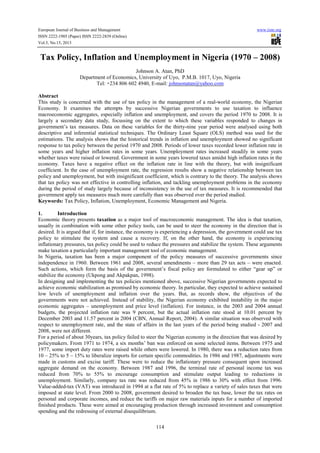
INF = Inflation Rate

Vol.5, No.15, 2013
125
ED = External Debt
BOP = Balance of Payments
ATR = Average Tax Rate
MSG = Money Supply Growth Rate
NFO = Net Foreign Operation
OPN = Openness of the Economy
IMP = Imports
EXP = Exports
UN = Unemployment Rate
CEXP = House Consumption Expenditure
Sources:
(1) National Bureau of Statistics, General household Survey Report 1995 – 2005
(2) Federal Office of Statistics, annual Abstract of Statistics (various issues)
(3) CBN Statistical Bulletin (various issues)
(4) CBN Annual Reports and Statement of Accounts (various issues)
(5) World Development Report (2007)
APPENDIX II
Figure (a): Trend Graph of Inflation and Average Tax Rates
Source: Captured by the researcher from Appendix 1
0
100
200
300
400
500
1970 1975 1980 1985 1990 1995 2000 2005
ATR*100 INF

Vol.5, No.15, 2013
126
Figure (b): Trend graph of Unemployment and Average Tax Rate (ATR)
Source: Captured by the researcher from Appendix 1
APPENDIX III
Unit Root Test: augmented dickey-fuller test result
ADF Test Statistic 5% Critical
Variables
Variable Level 1st
Difference Level 1st
Difference Decision
INF -3.747207 - -2.941145 - 1 (0)*
ATR -3.678830 - -2.954021 - 1 (0)*
EXCH 0.382891 -2.941145 -2.943427 -5.298530 1 (1)**
MSG 4.756677 - -2.954021 - 1 (0)*
OPN 3.473765 - -2.960411 - 1 (0)*
UN -1.3740776 -2.94445 -2.943427 -6.179655 1 (1)**
* = Stationary at levels
** = Stationary at first difference
Source: Researcher’s computation (2011)
0
4
8
12
16
20
1970 1975 1980 1985 1990 1995 2000 2005
ATR UN

Vol.5, No.15, 2013
127
APPENDIX IV
Cointegration test results based on Johansen Maximum Likelihood Procedure
(a) Inflation Equation
Unrestricted Cointegration Rank Test (Trace)
Hypothesized Trace 0.05
No. of CE(s) Eigenvalue Statistic Critical Value Prob.**
None * 0.772402 115.9119 69.81889 0.0000
At most 1 * 0.551965 61.14543 47.85613 0.0018
At most 2 * 0.318984 31.43873 29.79707 0.0321
At most 3 * 0.218187 17.22446 15.49471 0.0272
At most 4 * 0.196989 8.117292 3.841466 0.0044
Trace test indicates 5 cointegrating eqn(s) at the 0.05 level
* denotes rejection of the hypothesis at the 0.05 level
**MacKinnon-Haug-Michelis (1999) p-values
Unrestricted Cointegration Rank Test (Maximum Eigenvalue)
Hypothesized Max-Eigen 0.05
None * 0.772402 54.76649 33.87687 0.0001
At most 1 * 0.551965 29.70670 27.58434 0.0263
At most 2 0.318984 14.21427 21.13162 0.3477
At most 3 0.218187 9.107164 14.26460 0.2773
At most 4 * 0.196989 8.117292 3.841466 0.0044
Max-eigenvalue test indicates 2 cointegrating eqn(s) at the 0.05 level

Vol.5, No.15, 2013
128
(b) Unemployment Equation
Unrestricted Cointegration Rank Test (Trace)
Hypothesized Trace 0.05
None * 0.824525 153.7848 95.75366 0.0000
At most 1 * 0.636933 89.39527 69.81889 0.0006
At most 2 * 0.457286 51.90801 47.85613 0.0198
At most 3 0.386447 29.29464 29.79707 0.0570
At most 4 0.245897 11.22056 15.49471 0.1983
At most 5 0.020812 0.778176 3.841466 0.3777
Trace test indicates 3 cointegrating eqn(s) at the 0.05 level
Unrestricted Cointegration Rank Test (Maximum Eigenvalue)
Hypothesized Max-Eigen 0.05
None * 0.824525 64.38954 40.07757 0.0000
At most 1 * 0.636933 37.48726 33.87687 0.0177
At most 2 0.457286 22.61337 27.58434 0.1906
At most 3 0.386447 18.07408 21.13162 0.1271
At most 4 0.245897 10.44238 14.26460 0.1845
At most 5 0.020812 0.778176 3.841466 0.3777
Max-eigenvalue test indicates 2 cointegrating eqn(s) at the 0.05 level
APPENDIX V
(a) Equation 3.1: Inflation Equation Result
Variable Coefficient Std. Error t-Statistic Prob.
C 15.60713 5.774232 2.702893 0.0109
ATR -4.397694 4.226856 -1.040417 0.3059
EXCH 0.191264 0.163919 1.166817 0.2519
MSG -0.005661 0.191233 -0.029603 0.9766
OPN -1.413920 1.073756 -1.316798 0.1973
INF(-1) 0.395624 0.177996 2.222662 0.0334
R-squared 0.275893 Mean dependent var 21.01737
Adjusted R-squared 0.162751 S.D. dependent var 18.79753
S.E. of regression 17.19999 Akaike info criterion 8.671634
Sum squared resid 9466.870 Schwarz criterion 8.930200
Log likelihood -158.7610 F-statistic 2.438467
Durbin-Watson stat 1.954215 Prob(F-statistic) 0.055645

Vol.5, No.15, 2013
129
(b) Equation 3.2: Unemployment Equation
C 4.289731 0.845151 5.075700 0.0000
ATR -1.108544 0.568191 -1.951007 0.0599
EXCH 0.137307 0.022079 6.219015 0.0000
MSG -0.006023 0.022359 -0.269388 0.7894
OPN -0.297386 0.146331 -2.032283 0.0505
INF -0.016918 0.021841 -0.774592 0.4443
(c) Regression results of the first difference form (unemployment equation)
C -0.456598 0.359094 -1.271527 0.2130
D(ATR) -0.453087 0.423133 -1.070791 0.2925
D(EXCH) 0.177802 0.028214 6.301959 0.0000
D(MSG) 0.004377 0.017335 0.252504 0.8023
D(OPN) 0.203886 0.225601 0.903750 0.3731
D(INF) 0.015947 0.017049 0.935403 0.3568
Source: Researcher’s computation (2011)
APPENDIX VI
Correlation results
UNEMPLOYMENT EQUATION
UN ATR EXCH M2GDP OPN INF
UN 1.000000 0.655133 0.885981 0.758881 0.753973 -0.175565
ATR 0.655133 1.000000 0.812374 0.580775 0.692739 -0.244556
EXCH 0.885981 0.812374 1.000000 0.887940 0.907230 -0.192228
MGS 0.758881 0.580775 0.887940 1.000000 0.969847 -0.223479
OPN 0.753973 0.692739 0.907230 0.969847 1.000000 -0.261547
INF -0.175565 -0.244556 -0.192228 -0.223479 -0.261547 1.000000

This academic article was published by The International Institute for Science,
Technology and Education (IISTE). The IISTE is a pioneer in the Open Access
Publishing service based in the U.S. and Europe. The aim of the institute is
Accelerating Global Knowledge Sharing.
More information about the publisher can be found in the IISTE’s homepage:
http://www.iiste.org
CALL FOR PAPERS
The IISTE is currently hosting more than 30 peer-reviewed academic journals and
collaborating with academic institutions around the world. There’s no deadline for
submission. Prospective authors of IISTE journals can find the submission
instruction on the following page: http://www.iiste.org/Journals/
The IISTE editorial team promises to the review and publish all the qualified
submissions in a fast manner. All the journals articles are available online to the
readers all over the world without financial, legal, or technical barriers other than
those inseparable from gaining access to the internet itself. Printed version of the
journals is also available upon request of readers and authors.
IISTE Knowledge Sharing Partners
EBSCO, Index Copernicus, Ulrich's Periodicals Directory, JournalTOCS, PKP Open
Archives Harvester, Bielefeld Academic Search Engine, Elektronische
Zeitschriftenbibliothek EZB, Open J-Gate, OCLC WorldCat, Universe Digtial
Library , NewJour, Google Scholar

Tax policy, inflation and unemployment in nigeria (1970 – 2008)

Recomendados

Recomendados

Más contenido relacionado

La actualidad más candente

La actualidad más candente (18)

Similar a Tax policy, inflation and unemployment in nigeria (1970 – 2008)

Similar a Tax policy, inflation and unemployment in nigeria (1970 – 2008) (20)

Más de Alexander Decker

Más de Alexander Decker (20)

Último

Último (20)

Tax policy, inflation and unemployment in nigeria (1970 – 2008)