
Recomendados
Más contenido relacionado
La actualidad más candente
Destacado
Destacado (20)
Similar a Charting in excel
Similar a Charting in excel (20)
Charting in excel
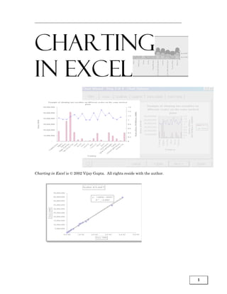
- 1. Charting in Excel Charting in Excel is 2002 Vijay Gupta. All rights reside with the author. 1
- 2. Charting in Excel Charting in Excel Charting in Excel Volume 2 in the series Excell for Professiionalls Exce for Profess ona s Volume 1: Excel For Beginners Volume 2: Charting in Excel Volume 3: Excel-- Beyond The Basics Volume 4: Managing & Tabulating Data in Excel Volume 5: Statistical Analysis with Excel Volume 6: Financial Analysis using Excel Published by VJ Books Inc All rights reserved. No part of this book may be used or reproduced in any form or by any means, or stored in a database or retrieval system, without prior written permission of the publisher except in the case of brief quotations embodied in reviews, articles, and research papers. Making copies of any part of this book for any purpose other than personal use is a violation of United States and international copyright laws. First year of printing: 2002 Date of this copy: Monday, December 16, 2002 This book is sold as is, without warranty of any kind, either express or implied, respecting the contents of this book, including but not limited to implied warranties for the book's quality, performance, merchantability, or fitness for any particular purpose. Neither the author, the publisher and its dealers, nor distributors shall be liable to the purchaser or any other person or entity with respect to any liability, loss, or damage caused or alleged to be caused directly or indirectly by the book. This book is based on Excel versions 97 to XP. Excel, Microsoft Office, Microsoft Word, and Microsoft Access are registered trademarks of Microsoft Corporation. Publisher: VJ Books Inc, Canada Author: Vijay Gupta 2
- 3. ABOUT THE AUTHOR Vijay Gupta has taught statistic, econometrics, and finance to institutions in the US and abroad, specializing in teaching technical material to professionals. He has organized and held training workshops in the Middle East, Africa, India, and the US. The clients include government agencies, financial regulatory bodies, non-profit and private sector companies. A Georgetown University graduate with a Masters degree in economics, he has a vision of making the tools of econometrics and statistics easily accessible to professionals and graduate students. His books on SPSS and Regression Analysis have received rave reviews for making statistics and SPSS so easy and “non-mathematical.” The books are in use by over 150,000 users in more than 140 nations. He is a member of the American Statistics Association and the Society for Risk Analysis. In addition, he has assisted the World Bank and other organizations with econometric analysis, survey design, design of international investments, cost-benefit, and sensitivity analysis, development of risk management strategies, database development, information system design and implementation, and training and troubleshooting in several areas. Vijay has worked on capital markets, labor policy design, oil research, trade, currency markets, and other topics. 3
- 4. Charting in Excel VISION Vijay has a vision for software tools for Office Productivity and Statistics. The current book is one of the first tools in stage one of his vision. We now list the stages in his vision. Stage one: Books to Teach Existing Software He is currently working on books on word-processing, and report production using Microsoft Word, and a booklet on Professional Presentations. The writing of the books is the first stage envisaged by Vijay for improving efficiency and productivity across the world. This directly leads to the second stage of his vision for productivity improvement in offices worldwide. Stage two: Improving on Existing Software The next stage is the construction of software that will radically improve the usability of current Office software. Vijay’s first software is undergoing testing prior to its release in Jan 2003. The software — titled “Word Usability Enhancer” — will revolutionize the way users interact with Microsoft Word, providing users with a more intuitive interface, readily accessible tutorials, and numerous timesaving and annoyance-removing macros and utilities. He plans to create a similar tool for Microsoft Excel, and, depending on resource constraints and demand, for PowerPoint, Star Office, etc. 4
- 5. Stage 3: Construction of the first “feedback-designed” Office and Statistics software Vijay’s eventual goal is the construction of productivity software that will provide stiff competition to Microsoft Office. His hope is that the success of the software tools and the books will convince financiers to provide enough capital so that a successful software development and marketing endeavor can take a chunk of the multi- billion dollar Office Suite market. Prior to the construction of the Office software, Vijay plans to construct the “Definitive” statistics software. Years of working on and teaching the current statistical software has made Vijay a master at picking out the weaknesses, limitations, annoyances, and, sometimes, pure inaccessibility of existing software. This 1.5 billion dollar market needs a new visionary tool, one that is appealing and inviting to users, and not forbidding, as are several of the current software. Mr. Gupta wants to create integrated software that will encompass the features of SPSS, STATA, LIMDEP, EViews, STATISTICA, MINITAB, etc. Other He has plans for writing books on the “learning process.” The books will teach how to understand one’s approach to problem solving and learning and provide methods for learning new techniques for self- learning. 5
- 6. CONTENTS CHAPTER 1 UNDERSTANDING CHART TYPES 21 1.1 Chart categories – deciding what chart type to use 22 1.1.a The “base” trends / levels comparison charts 23 1.1.b Stacked comparison charts 24 1.1.c “100% Stacked“ comparison of percent shares chart 25 1.1.d Scatter charts 25 1.1.e Charts that depict the “% share of each category within a series” – Pie and Doughnut charts 26 1.1.f The “2-Y axis” charts for comparing trends in two series that have widely different scales of measurement 27 1.2 The three “Columns” of sub-types 27 CHAPTER 2 A “BASE” CHART (COLUMNS, BARS, LINES OR AREAS) 30 2.1 Step one– choosing the chart type and sub-type 31 2.1.a Choosing a chart sub-type 33 2.1.b The “rows” in the grid 34 2.1.c The Columns in the grid 35 2.2 Understanding the sub-types using the grid method 36 Tips on the rows and Columns within the grid 36 “If I make a mistake in choosing a chart type, then do I have to remake the chart from scratch?” 37 “I want to change the chart type for many charts I made earlier. Is there a quick method for achieving this change? 37 2.3 Step two– Editing / choosing the data used in the chart 44 2.3.a Solution to the problem of Excel choosing the cell references (the data for the chart) incorrectly 44 2.3.b Other commonly encountered problems with defining series 47 2.4 Step three– setting detailed options in a chart – Titles, axis, Legend, Gridlines, data labels and more 49 2.4.a Titles 50 Differences in the “Titles” dialog across chart types and sub-types 51 The Titles option in other chart types 52 2.4.b Axes 52 Differences in the “Axes” dialog across chart types and sub-types 53 The “axis” option in other chart types 53 6
- 7. Contents 2.4.c Gridlines 54 Differences in the “Gridlines” dialog across chart types and sub-types 55 The “Gridlines“ option in other chart types 55 2.4.d Legend 55 Differences in the “Legend” dialog across chart types and sub-types 56 2.4.e Data labels 56 Differences in the “Data labels” dialog across chart types and sub-types 58 The “Data labels” option in other chart types 58 2.4.f Data Table 59 Differences in the “Data table” dialog across chart types and sub-types 59 2.5 Step four: choosing the location where the chart should be placed 60 2.6 ‘Step 5’– introducing new features specific to each data series 62 CHAPTER 3 “STACKED“ & “100% STACKED“ CHARTS 64 3.1 Stacked Charts 64 3.2 “100% Stacked“ charts 66 CHAPTER 4 SCATTER CHARTS 69 4.1 Step one: Selecting Chat Type & Sub-TYPE 69 4.2 Step two: Selecting the Source Data 70 4.2.a Comparing the procedural steps for this chart type to the analogous steps for making a Column chart 70 4.3 Step three: Setting Options 71 4.3.a Legend 71 4.3.b Titles 72 4.4 Step four: LocAtion 73 4.5 An extra step– adding a trend Line 74 CHAPTER 5 PIE AND DOUGHNUT CHARTS 79 5.1 Step one—selecting the data series 79 5.1.a Digression: Selecting data from non-adjacent rows / Columns 79 5.2 Step two: Data Source 81 5.3 Step three- the limited options for a Pie chart 82 5.4 Data labels: showing the percent share of each Slice 83 5.5 Step four 84 7
- 8. Charting in Excel 5.6 Converting a 2-Dimensional Pie into a 3-Dimensional Pie 85 5.7 Changing the 3-Dimensional view 87 CHAPTER 6 “2 Y-AXES“ CHARTS – CHARTING VARIABLES MEASURED ON DIFFERENT SCALES 90 6.1 Step one: choosing the data 90 6.2 Step two: setting the cell/data references for each Y-axis 92 6.2.a Solving a common problem – “Excel has failed to pick any series or the correct series for defining the X axis categories on the chart” 93 6.3 Step three: The options for the “Secondary Y-axis” 95 6.3.a Titles 96 6.4 The “2 Y Axes“ Line chart 98 CHAPTER 7 CHANGING A CHART 100 7.1 Changing the chart type 101 7.2 Changing the source data 103 7.3 Changing chart options 103 7.4 Changing chart location 104 7.5 Formatting the chart 105 7.6 How each step in chart creation creates and / or defines “objects” 105 Step one: choosing chart type 107 Step two: choosing the data series 107 Step three: Setting options 107 Step four: choosing the chart location 108 CHAPTER 8 FORMATTING CHARTS USING THE “OBJECT” MODEL APPROACH 110 8.1 The “Object Model” of a chart — the best way to understand a chart 110 Pie chart 117 8.2 When did you make all of these objects? 118 8.3 Objects created when formatting a data series 118 8.4 Objects created after the chart is made: “Trend Line“ 119 8
- 9. Contents 8.5 Data series specific objects created after the chart is made: Error Bars 120 CHAPTER 9 RESIZING, MOVING AND DELETING OBJECTS 123 9.1 Changing the size of an object 123 9.2 Moving objects 126 9.3 Deleting objects 128 C H A P T E R 1 0 “DRILL DOWN” FORMATTING APPROACH –LARGER TO SMALLER OBJECTS 130 10.1 The broad “area” objects (“Chart” and “Plot” area) 130 10.1.a Chart Area Object 130 10.1.a Plot Area object 135 10.1 The background objects – “Wall,” “Floor” and “Gridlines” 137 10.1.a Wall Object 137 Tips for formatting the “Wall“ object 139 10.1.b Floor Object 139 10.1.c Gridlines Object 140 10.1 The “Title” objects (text boxes) 142 10.1.a Chart Title Object 142 10.1.a Axis Title Object 147 10.2 Using the F4 key to save time and replicate formats 148 10.3 The “Legend“ objects 149 10.3.a Legend Object 149 Tips 150 10.3.b Legend Entry Object 151 10.1 Trend Line Object (within a Scatter, Line, Bar or Column chart) 152 10.2 Table option: (Data) Table Object 153 C H A P T E R 1 1 THE “AXIS” OBJECTS ATTACHED TO EACH AXES 157 11.1 Axis Object (Y-Axis or Value-Axis) 157 11.1.a Patterns 158 11.1.b Scale 159 11.2 Axis Object (X-Axis or Category-Axis) 161 11.2.a Patterns 161 9
- 10. Charting in Excel 11.2.b Scale 161 C H A P T E R 1 2 FORMATTING THE DATA SERIES AND DATA POINT OBJECTS 165 12.1 Labeling the data points: the “Data Points” and “Data Point” labels and Leader Lines 165 Data Labels Object for a data series (using the example of a Pie) 165 Data Label Object for each data point (using the example of a Pie) 168 Leader Lines and Leader Line object 170 C H A P T E R 1 3 DATA SERIES SPECIFICS ACROSS CHART TYPES AND SUB- TYPES 172 13.1 3-Dimensional Column charts 172 13.1.a Shape (only for 3-Dimensional Column / Bar) 173 13.1.b Chart Depth 174 13.1 2-Dimensional Column chart 175 13.2 2-Dimensional Line chart 176 Line pattern 177 13.2.a Drop Lines: available in all Line and area charts (but not in other chart types) 182 13.2.b High-low Lines and up-down Bars (only in a 2-Dimensional Line chart) 183 13.3 Stacked charts: options to stagger the ‘blocks’ and to have a “Series Line“ 183 13.3.a Staggering the blocks 185 13.3.b Adding a “Series line“ object to a data series in a Stacked Chart 185 13.4 Varying colors by data point 188 13.5 Doughnut hole size 189 13.6 3-Dimensional Pie chart 190 13.7 The ultimate drill-down object: Data Point Object 190 13.8 Y-Error Bars 192 13.9 X-Error Bars (unique to Scatter charts) 194 C H A P T E R 1 4 TIME SAVERS 197 14.1 The shortcut menu (using a right click on the mouse) 197 14.2 Customizing the short-cut “buttons” or “icons” in the Toolbar 199 10
- 11. Contents 14.2.a What is a Toolbar? 199 14.2.b Choosing a collection of icons that perform similar functions (for example, formatting) 200 14.2.c Understanding “Dynamic” Toolbars 201 Chart 201 Drawing and INSERT / PICTURE 201 14.2.d Placing / removing individual icons on / from the Toolbar 201 14.2.e Finding and selecting an icon 202 14.2.f Adding the selected icon onto the Toolbar 202 14.2.g Individual icons for broad charting features 203 Chart options icons 204 Individual icons for creating a new chart 204 C H A P T E R 1 5 FORMAT ONE CHART AND MAKE EXCEL APPLY THIS FORMAT TO OTHER CHARTS 207 15.1 Choosing the range whose format is desired as the “model” 207 15.2 Activating the format painter 207 C H A P T E R 1 6 SUMMARY TABLES 212 Mapping of menu options with sections of the book and in the series of books You may be looking for a section that pertains to a particular menu option in Excel. I now briefly lay out where to find (in the series) a discussion of a specific menu option of Excel. Table 1: Mapping of the options in the “FILE“ menu Menu Option Section that discusses the option OPEN Volume 1: Excel For Beginners SAVE SAVE AS SAVE AS WEB PAGE Volume 3: Excel– Beyond The Basics SAVE WORKSPACE Volume 3: Excel– Beyond The Basics 11
- 12. Charting in Excel Menu Option Section that discusses the option SEARCH Volume 1: Excel For Beginners PAGE SETUP Volume 1: Excel For Beginners This Book PRINT AREA Volume 1: Excel For Beginners PRINT PREVIEW Volume 1: Excel For Beginners PRINT Volume 1: Excel For Beginners PROPERTIES Volume 1: Excel For Beginners Table 2: Mapping of the options in the “EDIT“ menu Menu Option Section that discusses the option UNDO Volume 1: Excel For Beginners REDO Volume 1: Excel For Beginners CUT Volume 1: Excel For Beginners COPY PASTE OFFICE CLIPBOARD Volume 1: Excel For Beginners PASTE SPECIAL Volume 3: Excel– Beyond The Basics FILL Volume 4: Managing & Tabulating Data in Excel CLEAR Volume 1: Excel For Beginners DELETE SHEET Volume 1: Excel For Beginners MOVE OR COPY SHEET Volume 1: Excel For Beginners FIND Volume 1: Excel For Beginners REPLACE Volume 1: Excel For Beginners GO TO Volume 3: Excel– Beyond The Basics LINKS Volume 3: Excel– Beyond The Basics 12
- 13. Contents Menu Option Section that discusses the option OBJECT Volume 3: Excel– Beyond The Basics Volume 2: Charting in Excel Table 3: Mapping of the options in the “VIEW“ menu Menu Option Section that discusses the option NORMAL Volume 1: Excel For Beginners PAGE BREAK PREVIEW Volume 1: Excel For Beginners TASK PANE Volume 1: Excel For Beginners TOOLBARS Volume 1: Excel For Beginners Volume 3: Excel– Beyond The Basics FORMULA BAR Leave it on (checked) STATUS BAR Leave it on (checked) HEADER AND FOOTER Volume 1: Excel For Beginners COMMENTS Volume 3: Excel– Beyond The Basics FULL SCREEN Volume 1: Excel For Beginners ZOOM Volume 1: Excel For Beginners Table 4: Mapping of the options in the “INSERT“ menu Menu Option Section that discusses the option CELLS Volume 1: Excel For Beginners ROWS Volume 1: Excel For Beginners COLUMNS Volume 1: Excel For Beginners WORKSHEETS Volume 1: Excel For Beginners CHARTS This Book PAGE BREAK Volume 1: Excel For Beginners FUNCTION Volume 1: Excel For Beginners 13
- 14. Charting in Excel Menu Option Section that discusses the option FUNCTION/FINANCIAL Volume 6: Financial Analysis using Excel FUNCTION/STATISTICAL Volume 5: Statistical Analysis with Excel FUNCTION/LOGICAL Volume 3: Excel– Beyond The Basics FUNCTION/TEXT Volume 3: Excel– Beyond The Basics FUNCTION/INFORMATION Volume 3: Excel– Beyond The Basics FUNCTION/LOOKUP Volume 3: Excel– Beyond The Basics FUNCTION/MATH & TRIG Volume 3: Excel– Beyond The Basics FUNCTION/ENGINEERING Volume 3: Excel– Beyond The Basics FUNCTION/DATABASE Volume 3: Excel– Beyond The Basics FUNCTION/DATE & TIME Volume 3: Excel– Beyond The Basics NAME Volume 1: Excel For Beginners COMMENT Volume 3: Excel– Beyond The Basics PICTURE Volume 2: Charting in Excel DIAGRAM Volume 2: Charting in Excel OBJECT Volume 3: Excel– Beyond The Basics HYPERLINK Volume 3: Excel– Beyond The Basics Table 5: Mapping of the options inside the “FORMAT“ menu Menu Option Section that discusses the option CELLS Volume 1: Excel For Beginners ROW Volume 1: Excel For Beginners COLUMN Volume 1: Excel For Beginners SHEET Volume 1: Excel For Beginners AUTOFORMAT Volume 1: Excel For Beginners CONDITIONAL FORMATTING Volume 3: Excel– Beyond The Basics 14
- 15. Contents Menu Option Section that discusses the option STYLE Volume 1: Excel For Beginners Table 6: Mapping of the options inside the “TOOLS“ menu Menu Option Section that discusses the option SPELLING Volume 1: Excel For Beginners ERROR CHECKING Volume 3: Excel– Beyond The Basics SPEECH Volume 4: Managing & Tabulating Data in Excel SHARE WORKBOOK Volume 3: Excel– Beyond The Basics TRACK CHANGES Volume 3: Excel– Beyond The Basics PROTECTION Volume 3: Excel– Beyond The Basics ONLINE Volume 3: Excel– Beyond The Basics COLLABORATION GOAL SEEK Volume 6: Financial Analysis using Excel SCENARIOS Volume 6: Financial Analysis using Excel AUDITING Volume 3: Excel– Beyond The Basics TOOLS ON THE WEB The option will take you to a Microsoft site that provides access to resources for Excel MACROS In upcoming book on “Macros for Microsoft Office” ADD-INS Volume 6: Financial Analysis using Excel AUTOCORRECT Volume 1: Excel For Beginners Volume 4: Managing & Tabulating Data in Excel CUSTOMIZE Volume 3: Excel– Beyond The Basics OPTIONS Volume 1: Excel For Beginners Table 7: Mapping of the options inside the “DATA” menu Menu Option Section that discusses the option SORT Volume 4: Managing & Tabulating Data in Excel 15
- 16. Charting in Excel Menu Option Section that discusses the option FILTER Volume 4: Managing & Tabulating Data in Excel FORM Volume 4: Managing & Tabulating Data in Excel SUBTOTALS Volume 4: Managing & Tabulating Data in Excel VALIDATION Volume 4: Managing & Tabulating Data in Excel TABLE Volume 6: Financial Analysis using Excel CONSOLIDATION Volume 6: Financial Analysis using Excel GROUP AND OUTLINE Volume 1: Excel For Beginners PIVOT REPORT Volume 4: Managing & Tabulating Data in Excel EXTERNAL DATA Volume 4: Managing & Tabulating Data in Excel Table 8: Mapping of the options inside the “WINDOW“ menu Menu Option Section that discusses the option HIDE Volume 3: Excel– Beyond The Basics SPLIT Volume 1: Excel For Beginners FREEZE PANES Volume 1: Excel For Beginners Table 9: Mapping of the options inside the “HELP“ menu Menu Option Section that discusses the option OFFICE ASSISTANT Volume 1: Excel For Beginners HELP Volume 1: Excel For Beginners WHAT’S THIS Volume 1: Excel For Beginners 16
- 17. Contents INTRODUCTION Making charts • Chapter 1 on page 21 provides a framework for categorizing chart types and sub-types, teaches how to make different types of charts and introduces the concept of the “parts of a chart“ and the “object model.” These concepts are essential to understanding how to edit and format charts. • Chapter 2 on page 30 teaches demonstrates the four steps involved in making any chart, irrespective of the chart type. It uses the example of a Column chart. • Chapter 3 on 64 teaches how to make a “Stacked” chart -- in which each column/bar represents “shares” of data series • Chapter 4 on page 69 teaches how to make a Scatter chart. You also learn how to add a trend Line (Regression or other trend). • Chapter 6 on page 90 teaches the most difficult chart type – “2 Y- Axis charts.” In this chart type, one Y-axis represents one series and the other Y-axis another series that may use a different scale. Such charts are useful if, say, you want to show “Income Level (in dollars)” and “Income Growth Rate (in percentage),” both on the same chart. • Chapter 7 on page 100 teaches the quick modification of an existing chart. Formatting charts • Chapter 8 on page 110 lays the basis for learning how to format charts using the “object approach.” 17
- 18. Charting in Excel • Chapter 9 on page 123 shows how to resize, move, and edit charting objects. • Chapter 10 on page 130 is the first chapter in a sequence of “top to bottom” (or “largest to smallest”) object-based “drill down” process of formatting a chart1. • Chapter 11 on page 157 teaches the formatting and scaling of an extremely important set of objects – the Axes. It is placed in its own chapter because of its “more than cosmetic” role in a chart. • Chapter 12 on page 165 shows how to format the “Data Series” (for example, a line in a Line chart) object and a “Data Point” object. These objects need special emphasis because: (a) These are the ultimate “drilled down” objects. They represent the ultimate depiction of the data. (b) These objects differ across chart types. (c) When formatting these objects, you can create new “objects” – essentially, you can add very specific features that cannot be created any other way. (For example, “Error Bars“ or “Leader Lines to connect a Pie slice to the label for the slice.”) • Chapter 13 on page 172 dwells further on the difference in the Data Series and Data Point objects across different chart types. 1 The “drill down” starts from the largest object in a chart (the “Chart Area“) to the smallest (each “Data Point” on the plot.) This approach will make you a master in learning any other object based graphical software like PowerPoint. 18
- 19. Contents Time saving tools • Chapter 14 on page 197 shows how to use customization and short cut menus to save time when working on charts. • Chapter 15 on page 207 shows the use of two great tools for saving time in formatting charts – the Redo feature and the “Format Painter.” • Chapter 16 on 212 provides summary tables that you can use as quick reference guides. Sample data All the data files are included in the zipped file. 19
- 20. 20
- 21. Chapter 1: Understanding chart types CHAPTER 1 UNDERSTANDING CHART TYPES This book presents a radically different perspective on understanding the charting facility in Excel. You will learn to see a chart as an “object” made up of several “Sub-objects.” The trick to making, editing, and formatting charts is to be able to identify and work on each object within the chart. Open the sample file “Charts File1.xls.” This chapter provides a framework for categorizing chart types and sub- types, teaches how to make different types of charts and introduces the concept of the “parts of a chart“ and the “object model.” These concepts are essential to understanding how to edit and format charts. Section 1.1 on page 22 provides a framework for categorizing the many chart types2 into four main categories. Once you learn how to make a chart within one category, it will be easy to make other charts that are part of the same category. (For example, once you learn how to make a Column chart you will find it easy to make Bar, Cylinder, Cone, and Area charts.) If you look at the left half of the dialog shown in the next figure, you will view many different chart types. I will reclassify them within a few categories. 2A chart “type” identifies the way data is shown by the chart and the markers used for showing the data. An Excel chart shows data in four main ways. Different markers may be used to show data in one way. For example, the Pie and Doughnut chart types use different markers – Pie Slices and Doughnut Slices – to show the “percent share of each value of the sum of values of the series.” 21
- 22. Charting in Excel Within this Chapter, you will learn how to resolve some often-encountered problems with defining the correct data series for a chart. Section 2.3.a on page 44 shows the way around an exasperating problem– when Excel does not pick up the X-axis series (or any other series) while making a chart. Figure 1: The “Chart Wizard“ 1.1 CHART CATEGORIES – DECIDING WHAT CHART TYPE TO USE In Excel, you can make several types of charts. In terms of functionality, these charts can be broken down into four basic groups3. Within each 3 Strictly speaking, one may argue that there are more than six main categories. I concentrate on the six categories that are used often. 22
- 23. Chapter 1: Understanding chart types group, the different chart types depict information using different markers and formats. Once you learn how to make charts of one type within a group, you can easily make other chart types within that group. I now define each of these six basic groups, show an example of a chart from each group, and list the chart types that correspond to each group. 1.1.A THE “BASE” TRENDS / LEVELS COMPARISON CHARTS These chart types depict and compare the differences in values across series and trends in series. One can further divide this category into two– 1. The “Bar-type” charts for comparing individual data points. These include chart types like Column, Bar, Cylinder, Cone, Pyramid, Tubes, etc. The next figure shows this type of a chart. 2. The “Line-type” charts for comparing trends in different series. These include charts like Line, Area, etc. Open the sample file –”Charts File1.xls.” You will view examples of several of basic charts– • Chart “Basic Column” • Chart “Basic Bar“ • Chart “Basic Line“ • Chart “Basic Area” A column chart is reproduced in the next figure -- Chapter 2 teaches how to make this type of a chart. 23
- 24. Charting in Excel Figure 2: A Column chart 45000000 40000000 35000000 30000000 25000000 20000000 15000000 10000000 5000000 0 Iran, Islamic Rep. United Arab Emirates Syrian Arab Republic Algeria Morocco Egypt, Arab Rep. Country Name Kuwait Libya Saudi Arabia Tunisia Bahrain Israel Yemen, Rep. Jordan Qatar Oman Lebanon Country 1.1.B STACKED COMPARISON CHARTS Charts showing data for each values of a series “Stacked“ in a single Column – a “Stacked” Column, Bar, Line or Area chart –Chapter 3 on page 64 teaches how to make this type of a chart. Figure 3: A “Stacked“ Column chart 35,00 0,00 0 30,00 0,00 0 25,00 0,00 0 20,00 0,00 0 15,00 0,00 0 10,00 0,00 0 5,00 0,00 0 - 19 95 20 00 20 10 A lgeria Morocco Tunisia 24
- 25. Chapter 1: Understanding chart types 1.1.C “100% STACKED“ COMPARISON OF PERCENT SHARES CHART Section 3.2 teaches how to make this type of a chart. Figure 4: A “100% Stacked“ Column chart. Each of the columns has a height of 100%. 1.1.D SCATTER CHARTS These charts capture the relation between variables. The charts under this category include XY (Scatter), Bubble, and Surface. The next figure shows this type of a chart-- Chapter 4 on page 69 discusses how to make this type of chart. 25
- 26. Charting in Excel Figure 5: A Scatter Chart The dots represent the scatter plot. The line is an estimated regression line 1.1.E CHARTS THAT DEPICT THE “% SHARE OF EACH CATEGORY WITHIN A SERIES” – PIE AND DOUGHNUT CHARTS The charts under this category include Pie and Doughnut charts. The next figure shows an example of a chart under this category-- Chapter 5 on page 79 discusses how to make this type of chart. Figure 6: A Pie Chart Each Slice of a Pie measures the percent share of that category in the sum of all categories 26
- 27. Chapter 1: Understanding chart types 1.1.F THE “2-Y AXIS” CHARTS FOR COMPARING TRENDS IN TWO SERIES THAT HAVE WIDELY DIFFERENT SCALES OF MEASUREMENT These include “Lines on 2-axis” and “Line-Column on 2-axis.” Section on page 90 discusses how to make this type of charts. The next figure shows this type of a chart. If you decide to change the chart type after making the chart, you can do it quickly. This feature is taught in Chapter 7 on page 100. Figure 7: A 2 Y-axis chart Example of showing two variables on different scales on the same vertical plane 60,000,000 1.6 1.4 50,000,000 Ratio (Data 2010/Data 2000) 1.2 40,000,000 1 Data 2010 30,000,000 0.8 0.6 20,000,000 0.4 10,000,000 0.2 - 0 ria Jo l co ar a an n, rab in an Le ait Em sia e n . R bia ic . . Tu c s e ep la Rep ep by li m ate am no ra Ira , A hra at ub oc w ge m rd ni ab Ara R ,R Li Is ba Sa Q Ku O ir N or ep Al yp Ba en ry M m n udi nt ab ou Ye Is t Ar Ar C Eg d ria te ni Sy U 1.2 THE THREE “COLUMNS” OF SUB-TYPES 1. Basic 2. Stacked 27
- 28. Charting in Excel 3. 100% Stacked Figure 8: Understanding the sub-types of a Column chart Column 3: “100% Column 2: Stacked” column chart Stacked or cumulative column chart Column 1: Basic column chart 28
- 29. Page for notes 29
- 30. Charting in Excel CHAPTER 2 A “BASE” CHART (COLUMNS, BARS, LINES OR AREAS) Open the sample file “Charts File1.xls.” Assume you want a chart that captures the levels and trends across countries and years for the data in cells B1 to D19. To make this type of a chart, select the data cells B1 to D19 – Figure 9 shows this range. (Column B has the labels for the X-axis; Columns C and D have the data for the two sets of Columns.) Figure 9: The sample data Then choose the menu option INSERT / CHART (as shown in the next figure) or click on the chart icon shown in Figure 11. 30
- 31. Chapter 2: A “Base” Chart (Columns, Bars, Lines or Areas) Figure 10: The “Chart” menu option Figure 11: The INSERT / CHART icon Excel launches the “Chart Wizard.” (Figure 12 shows the first dialog within the wizard.) This wizard has four steps / dialogs. A “Wizard,” within the context of software, is a series of dialogs used for processes that need multiple dialogs. A wizard typically has the buttons “Next,” “Back,” and “Finish.” These buttons allow you to move to the next dialog, the previous dialog and to finish the process, respectively. You should be able to separate out the four steps in the chart wizard by the end of this Chapter. 2.1 STEP ONE– CHOOSING THE CHART TYPE AND SUB-TYPE In the first step (shown in Figure 12 to Figure 13), you select the type and sub-type of chart4. The left half of the dialog lists the chart types (as “Column,” “Bar,” “Line,” etc). Within each type of chart, you can select from one of the sub-types shown in the right half of the dialog. To choose a chart type and sub-type, first click on the name of a chart type on the left hand side of the dialog shown in Figure 12. Then, click on the picture of a chart sub-type on the right half of the same dialog. I chose 4 Note: "Custom Types" charts do not have any sub-types. 31
- 32. Charting in Excel the type “Column” as shown in the next figure5. I then moved my mouse over the area “Chart sub-type” and chose the sub-type highlighted in Figure 13. Figure 12: The two steps to choosing a chart type and sub-type Then, choose the chart sub-type by clicking on its picture in the right half. First, choose the chart type by clicking on its name in the left half. 5 In Chapter 7, I show how to quickly change the chart type and / or sub-type even after the chart has been made. 32
- 33. Chapter 2: A “Base” Chart (Columns, Bars, Lines or Areas) Figure 13: Selecting a sub-type. Note that Excel displays a short description of the currently selected sub-type. 2.1.A CHOOSING A CHART SUB-TYPE Let us dwell a bit further on the sub-types of a “Column” chart. Imagine the sub-types as cells in a table with each row and Column constituting one property. See Figure 13 and mentally partition the sub-types into three “rows” and three “Columns” as shown in the next figure. Figure 14: Categorizing the sub-types by using the grid method Row 1 Row 2 Row 3 Column 1 Column 2 Column 3 33
- 34. Charting in Excel View the sub-types. You should see similarities across all the sub-types in one row or Column. I briefly list the similarities below. 2.1.B THE “ROWS” IN THE GRID Row 1 sub-types (shown in the next figure) are all 2-Dimensional. Such charts are shown in Figure 21, Figure 23, and Figure 25. Figure 15: 2-Dimensional sub-types Row 2 sub-types (shown in the next figure) are all 3-Dimensional but they all show the data series next to each other unlike in row 3 sub-type. Such charts are shown in Figure 22 and Figure 24, Figure 16: 3-Dimensional sub-types with data series placed next to each other Row 3 sub-type (shown in the next figure) is 3-Dimensional with the different data series plotted in 3-dimensions (the series are placed one behind the other). Such a chart is shown in Figure 26. Figure 17: 3-Dimensional sub-type with data series placed one behind the other 34
- 35. Chapter 2: A “Base” Chart (Columns, Bars, Lines or Areas) 2.1.C THE COLUMNS IN THE GRID Column 1 sub-types (shown in the next figure) show the raw data for series next to each other (or one behind the other for row 3). Such charts are shown in Figure 21, Figure 22, and Figure 26. Figure 18: The column for “basic” charts Data Series “A” (light shade) Data Series “B” (darker shade) Column 2 sub-types (shown in the next figure) are “Stacked.” For any one case (in this specific example, any country) the different values are Stacked up, one over the other. Such a depiction is important when you want to [a] compare the sum of all the series at an X category, and [b] compare the relative shares of each series in the “total” value of the “stack” of Columns for each X category. Such charts are shown in Figure 23, Figure 24, and Chapter 3. Figure 19: The column for “Stacked“ chart sub-type. The height of each column is the Sum of data Series “A” and “B” . Data Series “A” (thick lines) Data Series “B” (thin dotted line) 35
- 36. Charting in Excel Column 3 sub-types (shown in the next figure) show the percentage shares of each series6 to the aggregate [sum] of the cases in a row. Such charts are shown in Figure 24 and Chapter 3. Figure 20: The column for “100% Stacked“ chart sub-type Share of data series “A” within the The height total for the observation (thick lines) sums to 100% for each observation Share of data series “B” within the sum for each observation (thin non-dotted line) 2.2 UNDERSTANDING THE SUB-TYPES USING THE GRID METHOD Tips on the rows and Columns within the grid For most chart types, the rows differ mainly in the visual marker used to show each data point and the visual 3-Dimensional effect. Essentially, the differences across the rows allow for a different look, but not a different way of depicting the data For most chart types– 6 A Pie chart shows the percentage break-up only for only one series. If you want to show the percentage break-up separately for several series, then use this sub-type of a column-type chart instead of a Pie chart. 36
- 37. Chapter 2: A “Base” Chart (Columns, Bars, Lines or Areas) • The first row shows the data using 2-Dimensional markers while the second and third rows use three-Dimensional markers. • The Columns differ mainly in the way in which the chart compares across data series. • The first Column shows the data “as it is.” • The second Column shows the data for the different series “Stacked“ on top of each other for each X-axis observation. • The third Column shows the percentage share, for each data series, of each data point's value of the number obtained if the data for one X-axis observation were added across all series. Understand the sub-types by using this grid method. Then choose which type suits your needs the best. If after you have made a chart, you want to change the type / subtype, it is very easy (as shown Chapter 7 on page 100). “If I make a mistake in choosing a chart type, then do I have to remake the chart from scratch?” No. (See Chapter 7 on page 100.) “I want to change the chart type for many charts I made earlier. Is there a quick method for achieving this change? Yes. You can change the chart type and sub-type using the CHART / CHART TYPE menu option. (See Chapter 7 on page 100.) The charts of the different sub-types are shown in sample file “Charts File1b Chart Sub Categories.xls.” 37
- 38. Charting in Excel Using the “grid” • Row 1 implies 2-dimensional chart • Column 1 implies a simple trend comparison Figure 21: The grid – example of a chart of sub-type (Row 1, Column 1) 5.E+07 Basic column chart 4.E+07 Data 1995 Data 2000 3.E+07 Number 2.E+07 1.E+07 0.E+00 ar el a an t ia an ria Em ia n co n a Al . p. p. ai en s ic ep by ai no bi ra r s at te m rd w Re Re oc bl ge ge ni hr ra ,R Li Is Q Y e ir a ba Ku O pu Jo Tu or Al Ba iA b ic Le ra Re M m ud Country m A la ab ab Sa t, Is yp Ar Ar n, Eg I ra n d r ia it e Un Sy Using the “grid” • Row 2 implies a 3-dimensional chart • Column 1 implies simple trend comparison 38
- 39. Chapter 2: A “Base” Chart (Columns, Bars, Lines or Areas) Figure 22: The grid – example of a chart of sub-type Row 2, Column 1 3D Columns -- Frontal View 5.E+07 4.E+07 Data 1995 Data 2000 3.E+07 Number 2.E+07 1.E+07 0.E+00 Algeria Egypt, Israel Kuwait Libya Oman Saudi Tunisia Yemen, Arab Arabia Rep. Rep. Country Using the “grid” • Row 1 implies a 2-dimensional chart • Column 2 implies a “Stacked“ chart 39
- 40. Charting in Excel Figure 23: The grid – example of a chart of sub-type Row 1, Column 2 Stacked column 9.E+07 8.E+07 7.E+07 Data 1995 Data 2000 6.E+07 Number 5.E+07 4.E+07 3.E+07 2.E+07 1.E+07 0.E+00 a r Jo l an an it Ba a r ia a n n co e ta a Al . by ri si wa ai ep m p. ra p. no bi ic m tes Om rd Qa ge ge oc ni hr Re Li Re Is ,R ra bl Ku ba Tu Al or ira pu iA Le en b ic M Em Ira Ara Re ud la Ye Sa Country ab ab t, Is yp Ar Ar n, Eg n d ria ite Un Sy Using the “grid” • Row 2 implies a 3-dimensional chart • Column 2 implies a “Stacked“ chart 40
- 41. Chapter 2: A “Base” Chart (Columns, Bars, Lines or Areas) Figure 24: The grid – example of a chart of sub-type Row 2, Column 2 3D Stacked Columns Data 1995 Data 2000 Yemen, Rep. 9.E+07 Tunisia 8.E+07 Saudi Arabia 7.E+07 6.E+07 Oman Number 5.E+07 Libya Country 4.E+07 Kuwait 3.E+07 Israel 2.E+07 Egypt, Arab Rep. 1.E+07 Algeria 0.E+00 41
- 42. Charting in Excel Figure 25: The grid – example of a chart of sub-type Row 1, Column 3 Distribution of Labor Force in North Africa 100% 90% Tunisia Tunisia Tunisia 80% 70% Morocco Morocco Morocco 60% 50% 40% 30% Algeria Algeria Algeria 20% 10% 0% 1995 2000 2010 42
- 43. Chapter 2: A “Base” Chart (Columns, Bars, Lines or Areas) Figure 26: The grid – example of a chart of sub-type Row 3, Column 1 Data 1995 Data 2000 Yemen, Rep. Tunisia Saudi Arabia Oman Libya Country 5.E+07 Kuwait 4.E+07 Number 3.E+07 Israel 2.E+07 Egypt, Arab Rep. 1.E+07 Algeria 0.E+00 Data 2000 Data 1995 Using the “grid” • Row 3 implies a 3-dimensional “building block” chart • Column 1 implies simple trend comparison Let me leave this digression and continue where I left off (refer to Figure 13 on page 33) After choosing the type of chart “Column” and the sub-type (“Row 2, Column 1” or “3-Dimensional Clustered“), click on “Next” (refer to Figure 12 and Figure 13 on page 33). 43
- 44. Charting in Excel 2.3 STEP TWO– EDITING / CHOOSING THE DATA USED IN THE CHART The second dialog of the “Chart Wizard“ will open. The dialog contains a sample preview of the chart. The “Data range” box has a reference to the data you selected for this chart. (This is shown in the next figure.) 2.3.A SOLUTION TO THE PROBLEM OF EXCEL CHOOSING THE CELL REFERENCES (THE DATA FOR THE CHART) INCORRECTLY In the area “Series in,” Excel has automatically “sensed” that the series is in rows. That is, the first row has the X-axis labels and the other rows have the data for each series. Each Bar in the chart represents one of the series in the rows “Data 1995” or “Data 2000.” However, we want the country names on the X-axis. Figure 27: Excel may incorrectly “sense” that the series are in rows when they might actually be in columns COMPARE THIS FIGURE WITH THE NEXT ONE. THE ONLY DIFFERENCE IN CHART CONSTRUCTION IS IN THE AREA “SERIES IN.” NOTE THE EFFECT OF CHOOSING “ROWS” INSTEAD OF “COLUMNS” --THE COUNTRY NAMES, WHICH ARE ON THE 44
- 45. Chapter 2: A “Base” Chart (Columns, Bars, Lines or Areas) To make this change- that is, to show that each Bar representing one of the Columns and not one of the rows, simply change the selection of “Series in” to “Columns” as shown in the next figure. Figure 28: The corrected definition of the sequence in which the data is to be broken into data series for charting This "preview" shows how the chart will look if you clicked on "Finish" at this stage. As you read this Chapter and practice, see how the sample preview changes to reflect the choices you make. Click on the tab “Series” at the top of the dialog. The options in here (the dialog is reproduced in the next figure) are the source of major problems in making charts. Therefore, I will go through them carefully. Focus on the area within the superimposed dark rectangle. Each name in the box “Series” defines one of the data series in the chart; furthermore, the data series is defined itself by the entries in the boxes “Name“ and “Values.” Click on the name “Series17“ in the box “Series.” 7 Excel should have picked up the names automatically but it failed; this happens often. In this Chapter, I try to mimic some of the common problems encountered in making charts in Excel. 45
- 46. Charting in Excel You can click on the “Name“ box, go back to the data, and click on the cell that has the series name, write in the name into the box “name,” or ignore the issue. Repeat this process for each data series. Figure 29: Understanding the “Chart Source Data” dialog of the chart wizard Each data series that will be represented in the chart is listed here. When you click on the name of a series, the cell references are the data series is shown in the box to the right of “Value.” If Excel has picked the name of the data series correctly from the first data point in each series, then the series name will be referenced in the box to the right of “Name.” Note that this box is empty. Excel frequently misses picking the series names, especially if the names are numbers (as they are in this example). If Excel has not picked up the name of a series from the first cell of the series (or if your series does not have labels in the first cell) then you can type the names manually. (These names provide the labels for the Legend that identifies each data series on the chart.) On the right side, type in a name for the series - say “1995 Data.” Leave the “Values” box as it is. The name of the data series will change from “Series1” to “1995 data” as shown in the next figure. 46
- 47. Chapter 2: A “Base” Chart (Columns, Bars, Lines or Areas) Figure 30: Manually typing in the label for a data series Following a similar process, define the name for “Series2.” Figure 31: Manually typing in the label for another data series 2.3.B OTHER COMMONLY ENCOUNTERED PROBLEMS WITH DEFINING SERIES Excel may not understand that the first Column in the data range for the chart is the series for the X-axis labels. Instead, Excel may pick up the X- axis series as a data series (that is, a Y-axis series) and not have any references for the X-axis. In this example, “Series3” is not a data series. However, Excel has mistakenly “sensed” that it is a data series. Instead of being in the “Series” box, “Series3” should define the X-axis category labels. The cell references for “Series3” should be in the box “Category (X) axis labels.” 47
- 48. Charting in Excel Figure 32: Removing a series from the “Chart Data Source” dialog Let us correct this frequently encountered mistake by Excel. “Series3” first has to be removed from the list of data series. To do this, click on the series name “Series3” and then click on the button “Remove.” Now, manually define the cell references for “Series3” as the list that will fill the X-axis. Click on the right edge of the box “Category (X) axis labels.” Figure 33: Adding a reference to the cells that have the title and labels for the X-axes Enter the range for the X-axis labels. You can type the range, or, after clicking on the edge of the box, go to the sheet with the data series and highlight the data. The “Category(X) axis labels” box will contain the cell references for the X series. (An example is shown in the next figure.) Click on the right edge of the box and Excel will return you to the main dialog for step two of the charting process. Figure 34: Example of the reference for the title and labels for the X-axis 48
- 49. Chapter 2: A “Base” Chart (Columns, Bars, Lines or Areas) Now the chart reads the X-axis and Y-axis series correctly as shown in the next figure. Let us get back from this digression. The series definitions are correct (as shown in the next figure). Click on the button “Next.” Figure 35: The “Chart Source Data” dialog has been filled correctly 2.4 STEP THREE– SETTING DETAILED OPTIONS IN A CHART – TITLES, AXIS, LEGEND, GRIDLINES, DATA LABELS AND MORE The third dialog of the chart wizard opens. .This is a multi-tabbed dialog (as is shown in the next figure) and permits the writing of Titles (for the chart and each axis), choosing to place / remove / position Legends and data labels, Gridline options, etc. 49
- 50. Charting in Excel The options differ widely depending upon the type of chart you are making. This will become apparent when I teach how to make Scatter, Pie and 2-axis charts. Figure 36: The third step in the chart wizard – the “Chart Options” dialog 2.4.A TITLES Click on the tab “Titles.” If you desire8, type in the text for “Chart Title“ and / or a Title for the “Category (X) Axis” and / or one for the “Value (Z) Axis.” The next figure provides an illustration. Note that once you have entered the text for the Titles, the sample preview of the chart will change on the right half of the dialog. (Look at the next figure-- notice that the Titles have been added in the sample 8 All the options in step 3 of the wizard are at your discretion. Excel will create some defaults for some of the options, but for many other options, like the titles, Excel will not create the object (in this case, each object is an axis title or the chart title) until you type some text into the relevant text boxes. 50
- 51. Chapter 2: A “Base” Chart (Columns, Bars, Lines or Areas) preview.) The thick arrows trace the Title text you enter into the preview of the chart.) Figure 37: Adding the Chart & Axes titles Differences in the “Titles” dialog across chart types and sub-types • Chart Title is available for all chart types and sub-types • Category (X) axis Title is not available for Pie and related chart types • Series (Y) axis Title is available for most chart types (except Pie and related chart types) if the chart sub-type is two- Dimensional • Value (Z) axis Title is only available for three-dimensional sub-types (except for 3-Dimensional Pie and related chart types) 51
- 52. Charting in Excel The Titles option in other chart types • Scatter chart “Titles“ options are shown in Figure 54 on page 73. • Pie chart “Titles“ options are shown in Chapter 5. • 2-Y axis chart “Titles“ options are shown in Chapter 6. The options include a “Secondary” Category (X) axis Title and a “Secondary” Value (Y) axis Title. 2.4.B AXES Click on the tab “Axes.” Figure 32 shows the dialog that opens. (Depending on the type of chart you are making, the options shown may differ, or there may not even be a tab “Axes” as in the case of a Pie chart – a Pie chart depicts only one series, and, hence, does not need an “Axes.”) Excel chooses the default axis; usually, you do not need to make any changes. The recommended choices are shown in Figure 38. You may want to play around with the options just to see what happens when you choose other options. (The sample preview will show the impact of each such change you make.) 52
- 53. Chapter 2: A “Base” Chart (Columns, Bars, Lines or Areas) Figure 38: Choosing the axes to display on the chart Differences in the “Axes” dialog across chart types and sub-types • Category (X) axis is not available for Pie and related chart types • Series (Y) axis is available for most chart types (except Pie and related chart types) if the chart sub-type is two- Dimensional • Value (Z) axis is only available for three-dimensional sub- types (except for 3-Dimensional Pie and related chart types) The “axis” option in other chart types • In Scatter charts, each axis is a value axis. Therefore, both the axis have formatting options that are equivalent to Y- axis in a Column chart. 53
- 54. Charting in Excel • Pie charts do not have an “Axes“ option • 2-Y axis chart “Axes“ options include a “Secondary” Category (X) axis and a “Secondary” Value (Y) axis. 2.4.C GRIDLINES Click on the tab “Gridlines.“ The dialog shown in Figure 39 will open. (Depending on the type of chart you are making, the “Gridlines” tab may not exist.) In this example, the default settings include only the “Value (Z) axis Major Gridlines.” (Depending on the chart type and sub-type, the default Gridlines may differ.) Experiment with the other options and see what happens. Usually too many Gridlines can make a chart difficult to read. Therefore, I advise minimizing on using Gridlines. Figure 39: Choosing gridlines 54
- 55. Chapter 2: A “Base” Chart (Columns, Bars, Lines or Areas) Differences in the “Gridlines” dialog across chart types and sub-types • Series (Y) Gridlines are available for most chart types (except Pie and related chart types) if the chart sub-type is two- Dimensional • Value (Z) Gridlines are only available for three-dimensional sub-types (except for 3-Dimensional Pie and related chart types) The “Gridlines“ option in other chart types • Pie charts do not have a “Gridlines“ option • 2-Y axis chart “Gridlines“ – the options include a “Secondary” Category (X) axis and a “Secondary” Value (Y) axis. 2.4.D LEGEND Click on the tab “Legend.” The dialog shown in the next figure opens. You have two options– selecting or deselecting the box next to “Show Legend.” Legends are essential in Column, Line, and similar charts (if the chart depicts more than one series on the Y and / or Z-axis). In (two variable) Scatters, Pie and some other chart types, Legends are superfluous. If you want to keep the Legend, then choose the placement (within the chart) of the box that contains the Legend keys. In the area “Placement,” choose one of the options. I show the result from choosing the placement option “Bottom.” Compare the sample previews– notice that the Legend is placed in different parts of the chart. 55
- 56. Charting in Excel Once the chart is completed, you can use the mouse to click-and-drag the Legend to any place on the chart. One good option is to click-and-drag to an empty area within the plot itself. This saves on space Figure 40: The best place to show the legend is the “Bottom” of the chart Differences in the “Legend” dialog across chart types and sub-types The Legend option is available for all chart types and sub-types • The dialog is the same for all chart types and sub-types • As mentioned earlier, in Pie, two-variable Scatters, and some other chart types, Legends are redundant. 2.4.E DATA LABELS Click on the tab “Data Labels.” Depending on the chart type, you will see different options of what kinds of labels can be chosen. If you choose 56
- 57. Chapter 2: A “Base” Chart (Columns, Bars, Lines or Areas) “Show Value,“ the chart will display the value of each Column in the chart! There are 38 Columns in this chart. Therefore, choosing “Show Values” may make the chart very cluttered as is shown in the sample preview (see the right half of the dialog shown in the next figure. Typically, you will not want any labels in this type of a chart. (As you will see later, such labels are essential for chart types like Pie.) “Show Label“ places the X-axis label (the country name in this example) on each Column. Try it out. Figure 41: Choosing to see labels and/or values for each data point 57
- 58. Charting in Excel Figure 42: The problem in choosing to see data labels if the chart has more than a few data points Unless you have very few data points, choose the option “None.” Differences in the “Data labels” dialog across chart types and sub-types Data labels are available for all chart types and sub-types but are of use in only certain chart types (like the Pie) or only when the number of data points and series is small. The “Data labels” option in other chart types Click on the right edge of the box and Excel will return you to the main dialog for chart types. Pie charts have the maximum options within the “Data labels” dialog. They provide the option of placing percentage values in the data labels – an extremely useful option because Pie and related chart types are typically used to compare the percent shares from a total. 58
- 59. Chapter 2: A “Base” Chart (Columns, Bars, Lines or Areas) 2.4.F DATA TABLE Click on the tab “Show Data Table.” If you choose “Show data table” then the data used in the chart will be placed in table format below the chart (as is shown the next figure). This can be an excellent way to make the charts more informative and to remove the need for making a table and a chart separately in your report. Figure 43: Choosing whether to include a table with the data used in the chart Usually you will not want the show the data table. So, deselect it (as shown in the next figure) and Execute this part of the wizard and move to the next step by clicking on the button “Next.” Differences in the “Data table” dialog across chart types and sub-types The data table option is not available for Pie, Scatter, and related chart types 59
- 60. Charting in Excel Figure 44: The third step in the chart making process is complete 2.5 STEP FOUR: CHOOSING THE LOCATION WHERE THE CHART SHOULD BE PLACED At this point, you are at the last step / dialog of the chart wizard. You have to choose where to place the chart you are making. I prefer to place it on its own sheet9 and therefore recommend choosing the option “as New Sheet” as shown in the next figure. All the steps in the wizard have been completed. 9 This has at least four advantages compared to the option "As object in”: (a) formatting is easier; (b) you see the chart as it will look when printed, (c) other drawing tools can be added with ease. (d) After formatting and refining the chart, you can always copy and paste the chart from its own sheet on to another sheet. 60