IOSR Journal of Electronics and Communication Engineering(IOSR-JECE) is an open access international journal that provides rapid publication (within a month) of articles in all areas of electronics and communication engineering and its applications. The journal welcomes publications of high quality papers on theoretical developments and practical applications in electronics and communication engineering. Original research papers, state-of-the-art reviews, and high quality technical notes are invited for publications.

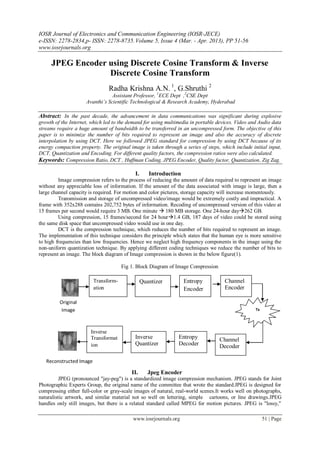
1. IOSR Journal of Electronics and Communication Engineering (IOSR-JECE)
e-ISSN: 2278-2834,p- ISSN: 2278-8735. Volume 5, Issue 4 (Mar. - Apr. 2013), PP 51-56
www.iosrjournals.org
JPEG Encoder using Discrete Cosine Transform & Inverse
Discrete Cosine Transform
Radha Krishna A.N. 1, G.Shruthi 2
Assistant Professor, 1ECE Dept ,2CSE Dept
Avanthi’s Scientific Technological & Research Academy, Hyderabad
Abstract: In the past decade, the advancement in data communications was significant during explosive
growth of the Internet, which led to the demand for using multimedia in portable devices. Video and Audio data
streams require a huge amount of bandwidth to be transferred in an uncompressed form. The objective of this
paper is to minimize the number of bits required to represent an image and also the accuracy of discrete
interpolation by using DCT. Here we followed JPEG standard for compression by using DCT because of its
energy compaction property. The original image is taken through a series of steps, which include initial input,
DCT, Quantization and Encoding. For different quality factors, the compression ratios were also calculated.
Keywords: Compression Ratio, DCT , Huffman Coding, JPEG Encoder, Quality factor, Quantization, Zig Zag.
I. Introduction
Image compression refers to the process of reducing the amount of data required to represent an image
without any appreciable loss of information. If the amount of the data associated with image is large, then a
large channel capacity is required. For motion and color pictures, storage capacity will increase momentously.
Transmission and storage of uncompressed video/image would be extremely costly and impractical. A
frame with 352x288 contains 202,752 bytes of information. Recoding of uncompressed version of this video at
15 frames per second would require 3 MB. One minute  180 MB storage. One 24-hour day262 GB.
Using compression, 15 frames/second for 24 hour1.4 GB, 187 days of video could be stored using
the same disk space that uncompressed video would use in one day.
DCT is the compression technique, which reduces the number of bits required to represent an image.
The implementation of this technique considers the principle which states that the human eye is more sensitive
to high frequencies than low frequencies. Hence we neglect high frequency components in the image using the
non-uniform quantization technique. By applying different coding techniques we reduce the number of bits to
represent an image. The block diagram of Image compression is shown in the below figure(1).
Fig 1. Block Diagram of Image Compression
Transform- Quantizer Entropy Channel
ation Encoder Encoder
Original
Image Tx
Channel
Inverse
Transformat Inverse Entropy Channel
ion Quantizer Decoder Decoder
Reconstructed Image
II. Jpeg Encoder
JPEG (pronounced "jay-peg") is a standardized image compression mechanism. JPEG stands for Joint
Photographic Experts Group, the original name of the committee that wrote the standard.JPEG is designed for
compressing either full-color or gray-scale images of natural, real-world scenes.It works well on photographs,
naturalistic artwork, and similar material not so well on lettering, simple cartoons, or line drawings.JPEG
handles only still images, but there is a related standard called MPEG for motion pictures. JPEG is "lossy,"
www.iosrjournals.org 51 | Page

2. JPEG Encoder using Discrete Cosine Transform & Inverse Discrete Cosine Transform
meaning that the decompressed image isn't quite the same as the one that started with. A useful property of
JPEG is that the degree of lossiness can be varied by adjusting compression parameters.
Figure 2.1 describes the JPEG process. JPEG divides the image into 8X8 pixel blocks and then
calculates the DCT of each block. A quantizer rounds off the DCT coefficients according to the quantization
matrix. This step produces the ―lossy‖ nature of JPEG, but allows for large compression ratios.
JPEG’s compression technique uses a variable length code on these coefficients, and then writes the
compressed data stream to an output file (*.jpg). For decompression JPEG recovers the quantized DCT
coefficients from the compressed data stream, takes the inverse transforms and displays the image.
Quantization Coding
Tables Tables
Headers
Spatial to DCT Discard Lossless
Tables
domain Unimportant coding
Input Transformation DCT domain of DCT
samples domain
Quantization samples Data
Fig 2.1 Block Diagram of JPEG Encoder
Entropy
III. D Dct/Idct Architecture AndencoderJpeg
The key to the JPEG compression is a mathematical transformation known as the Discrete Cosine
Transform (DCT). It also includes the well-known Fast Fourier Transform (FFT). Its basic operation is to take a
signal and transform it from one type of representation to another.
In this case the signal is a graphical image. The concept of this transformation is to transform a set of
points from the spatial domain into an identical representation in frequency domain. It identifies pieces of
information that can be effectively —thrown away without seriously reducing the image’s quality.
The mathematical function for a two-dimensional DCT is:
1 N 1 N 1
 (2 x  1)i   (2 y  1) j 
DCT (i, j )  C (i)C ( j )  pixol ( x, y)Cos  Cos   3.1
2N x 0 y 0  2N   2N 
1
C ( x)  If x is 0, else 1 if x > 0 3.2
2
The DCT operation is shown in the below example:
The input 8 x 8 matrix (Fig 3.1) from a gray-scale image consists of pixel values which are randomly
spread around 140 to 175 range. These values are fed to the DCT algorithm, creating the output matrix (Fig 3.2).
The output matrix consists of DCT Coefficients, which is ordered in a way that coefficients containing
useful and important data for representation of the image are in the upper left of the matrix and in the lower right
coefficients containing less useful information.
The DC coefficient (represented in bold as shown in fig 3.2) is at position (0, 0) in the upper left-hand
corner of the matrix and it represents the average of the other 63 values in the matrix. This step prepares the
image for the next step, namely quantization.
www.iosrjournals.org 52 | Page

3. JPEG Encoder using Discrete Cosine Transform & Inverse Discrete Cosine Transform
For decoding purpose there is an Inverse DCT (IDCT):
1 N 1 N 1
 (2 x  1)i   (2 y  1) j 
pixol ( x, y) 
2N
  C(i)C ( j)DCT (i, j)Cos 
i 0 j 0 
Cos
2N   2N 
  
3.4
1
C ( x)  if x is 0, else 1 if > 0 3.5
2
IV. Quantization & Entropy Coding
4.1 Quantization
Till now, in the JPEG compression, partial image compression has occurred. Of all the steps
quantization is the essence of lossy compression.
Quantization is a process of reducing the number of bits needed to store an integer value by reducing
the precision of the integer. For every element in the DCT matrix, a corresponding value in the quantization
matrix gives a quantum value. The quantum value is that which is stored in the compressed image.
The formula for quantization is:
DCT (i, j )
QuantizedValue (i, j )  , (Rounded to the nearest integer) 4.1
Quantum(i, j )
Selecting a quantization matrix must be done carefully. Although JPEG allows for the use of any
quantization matrix, ISO has done extensive testing and developed a standard set of quantization values that
cause impressive degrees of compression.
To calculate the quantization matrix we use this formula:
Quantization matrix Q (i, j) is: Q (i, j) = 1 + (1+i+j). (Quality Factor) 4.2
The next step in the JPEG process is coding the quantized images. This is done through following
steps: 1. Convert the DC coefficient to a relative value.
2. Reorder the DCT block in a zig-zag sequence as shown in fig 4.1.
Because so many coefficients in the DCT image are truncated to zero values during the coefficient
quantization stage, the zeros are handled differently than non-zero coefficients. They are coded using a Run-
Length Encoding (RLE) algorithm.
Fig 4.1: Zig-Zag sequence for Binary Encoding
4.2 Entropy Coding
Finally, the JPEG algorithm outputs the DCT block’s elements using an entropy encoding mechanism
that combines the principles of RLE and Huffman encoding. The output of the entropy encoder consists of a
sequence of three tokens, repeated until the block is complete.
The three tokens are:
(1) The run length, the number of consecutive zeros that precede the current zero element in the DCT output
matrix;
(2) The bit count, the number of bits used to encode the amplitude value that follows, as determined by the
Huffman encoding scheme; and
(3)The amplitude, the amplitude of the DCT coefficient
4.2.1 Coding the DC Coefficients
Firstly, we change the absolute value of the DC Coefficient at (0,0) to a relative value. Since adjacent
blocks in an image display a high degree of correlation, coding the DC element as the difference from the
previous DC element typically produces a very small number. This value is called the "DPCM difference" or the
"DIFF" DC coefficients are sent with differential coding and is given by Zi = DCi –DCi-1
www.iosrjournals.org 53 | Page

4. JPEG Encoder using Discrete Cosine Transform & Inverse Discrete Cosine Transform
4.2.2 Coding the AC Coefficients
AC coefficients are coded in Zigzag (called in ZZ in standard) order to maximize possible runs of
zeros. Code unit consist of run length followed by coefficient size. Baseline coding of size category is the same
as for DC differences.
The following two algorithms are used for Huffman coding:
I–Algorithm
1. JPEG DC Coefficient Code Word Finding (DPCM)
(1). DC Coefficient = - 9., (2).Cat=4 [10], (3).Base Code =101 and Length of code word=7[10]
(4) –9’s, Binary Code=0110 ------> it is called as LSB. (i.e., 9’s Binary Code=1001 and it is 1’s
compliment=0110 and Add 1 ==>0111 ==> again sub 1=0110). i.e. Binary Code =>1’s Comp+1=>sub
1==>LSB (if DC Coefficient –ve only other wise, we can take directly binary equavalent of DC Coefficeint
is LSB )
(5).Concatenate BC & LSB=CW from step 3 and 4
DC Code Word= 101 0110
II–Algorithm
2. JPEG AC Coefficient Code Word finding
(1). AC Coefficient = - 4, (2).Cat=3 [10], (3).run=0 from AC Coefficients Array; ==>run/Cat=0/3 ,(4).Base
Code for 0/3 is =100 [10], (5) –4’s, Binary Code=011 ------> it is called as LSB (4’s Binary Code=100 and its
1’s compliment=011and add 1=>100 again sub 1=011).i.e. Binary Code =>1’s Comp+1=>sub 1==>LSB (if AC
Coefficient –ve only other wise, we can take directly binary equavalent of AC Coefficeint is LSB ).
(6).Concatenate BC & LSB=CW from step 4 and 5
AC Code Word= 100 011
V. Software Implementation & Compression Ratio
This application is developed in "MATLAB" on windows run PC. The input image file was taken as a
BMP file of size 256x256 the output reconstructed image file also has the same size, but not the same quality,
i.e. with a little visible distortion. The input image and reconstructed image files are shown in the next section.
The Compression Ratio and Data Redundancy have been calculated for the compressed image data. As the
compression ratio is increased, the quality of the image decreases. This is the limitation of JPEG.
The following details are the results of JPEG Compression: Input image file, output compressed image
data, Reconstructed image, compression Ratio, Relative Data Redundancy are given below.
5.1 Input Image File Details
For implementation purpose, an image is considered, for which the source code has been written in
Matlab. The input image is taj.bmp. All input files are in bit map format (BMP). Images can be taken in any
format like bmp or JPEG.
5.1.1 Details of Image Space
Name of image : a1.bmp
Color type : color (24-bit color image)
Compression : no compression
Resolution : 96 pixels/inch
Size : 256 X 256 X 24
Units : pixels
Input image data : n1=1572864
Output compressed
Image data : n2=373601
Compression ratio : Cr = n1/n2=1572864/373601=4.21 i.e.
approximatey 4:1
5.2 Relative Data Redundancy
Now calculating relative data redundancy
Rd=1-1/cr, For image, Rd=1-1/cr, Rd=1-1/4=.75=75%.
Therefore, JPEG data now, 75% reduction i.e a compression ratio 4:1 means that the first data set has 4
information carrying units (say, bits) for every 1 unit in the second or compressed data set. The corresponding
redundancy of 0.75 implies that the 75% of the data in the first data sent is redundant.
www.iosrjournals.org 54 | Page

5. JPEG Encoder using Discrete Cosine Transform & Inverse Discrete Cosine Transform
VI. Result Analysis
In general, image compression means, by using less number of bits (compressing the bits) to
reconstruct the original image with little visible distortion. Due to this distortion, various parameters of original
image has changed Analysis of these parameters are shown in Table 1. The output result of reconstructed image
files are shown below which have the final result. The output image is same as input image, but with little
visible distortion as shown in the figures. The images of output files and input files have been enclosed. The
data redundencies for different compression ratios are shown in Table 6.1
Fig 6.1 Original Image Fig 6.2 Compressed Image with QF=6.5 Fig 6.3 Compressed Image with
QF=9
Fig 6.4 Compressed Image ,QF=14 Fig 6.5 Compressed Image, QF=19 Fig 6.6 Compressed Image,
QF=25
Fig 6.7 Compressed Image with QF=35 Fig 6.8 Compressed Image with QF=45
TABLE 1. Comparison of different parameters of the output results
S.No Fig Quality Actual Compressed Compression Data
Name Factor Length Length Ratio Redundancy(%)
1 Fig 6.1 --- 192 KB --- --- -
2 Fig 6.2 6.5 192 KB 14.626 KB 13.13 92.3
3 Fig 6.3 9.0 192 KB 11.589 KB 16.57 93.9
4 Fig 6.4 14 192 KB 8.573 KB 22.40 95.5
5 Fig 6.5 19 192 KB 7.075 KB 27.51 96.3
6 Fig 6.6 25 192 KB 6.018 KB 31.91 96.8
7 Fig 6.7 35 192 KB 5.065 KB 37.90 97.3
8 Fig 6.8 45 192 KB 4.486 KB 42.80 97.6
www.iosrjournals.org 55 | Page

6. JPEG Encoder using Discrete Cosine Transform & Inverse Discrete Cosine Transform
VII. Conclusion And Future Scope
Image compression is an extremely important part of modern computing. By having the ability to
compress images to a fraction of their original size, valuable (and expensive) disk space can be saved. In
addition, transportation of images from one computer to another becomes easier and less time consuming
(which is why image compression has played such an important role in development of the internet). The JPEG
image compression algorithm proves as a very effective way to compress images with minimal loss in quality.
This work can be extended to compress the images by using the JPEG encoder for FPGA implementation by
using suitable hardware. Using the Verilog HDL coding, the results may be compared with the above outputs
which are implemented by using MATLAB. The accurate results may be noticed in terms of cost and power
consumption.
References
[1] W. B. Pennebaker and J. L. Mitchell, ―JPEG – Still Image Data Compression Standard,‖ Newyork: International Thomsan
Publishing, 1993.
[2] G. Strang, ―The Discrete Cosine Transform,‖ SIAM Review, Volume 41, Number 1, pp. 135-147, 1999.
[3] R. J. Clark, ―Transform Coding of Images,‖ New York: Academic Press, 1985.
[4] A. K. Jain, ―Fundamentals of Digital Image Processing,‖ New Jersey: Prentice Hall Inc., 1989.
[5] A. C. Hung and TH-Y Meng, ―A Comparison of fast DCT algorithms,‖ Multimedia Systems, No. 5 Vol. 2, Dec 1994.
[6] G. Aggarwal and D. D. Gajski, ―Exploring DCT Implementations,‖ UC Irvine, Technical Report ICS-TR-98-10, March 1998.
[7] J. F. Blinn, ―What's the Deal with the DCT,‖ IEEE Computer Graphics and Applications, July 1993, pp.78-83.
[8] Spiliotopoulos V, Zervas N.D, Androulidakis C.E, Anagnostopoulos G, and Theoharis S, ―Quantizing the 9/7 Daubechies Filter
Coefficients for 2D-DCT VLSI Implementations," in 14th International Conference on Digital Signal Processing, 2002, vol. 1,
pp. 227-231.
[9] Larry Rowe, ―Image Quality Computation," Available Online: http://bmrc. berkeley. Edu / courseware/cs294 / fall97 /
assignment/ psnr.html.
[10] Rafael C. Gonzalez and Richard E. Woods, ― Digital Image Processing‖ Addison-Wesley, Fifth Indian Reprint – 2000.
www.iosrjournals.org 56 | Page