
Recomendados
Recomendados
Más contenido relacionado
La actualidad más candente
La actualidad más candente (14)
Similar a ROOTS OF EQUATION GRAPHICAL ANALYSIS
Similar a ROOTS OF EQUATION GRAPHICAL ANALYSIS (20)
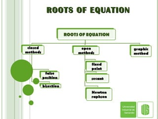
ROOTS OF EQUATION GRAPHICAL ANALYSIS
- 2. Graphical analysis is the simplest method for obtaining results in both life data and accelerated life testing analyses. Although they have limitations in general graphical methods are easily implemented and easy to interpret. The graphical method for estimating the parameters of accelerated life data involves generating two types of plots. First, the life data at each individual stress level are plotted on a probability paper appropriate to the assumed life distribution. GRAPHIC METHOD this method is very simple and is well known to better illustrate , i will make an example.
- 4. The bisection method is a root-finding algorithm which repeatedly bisects an interval then selects a subinterval in which a root must lie for further processing. It is a very simple and robust method, but it is also relatively slow. The method is applicable when we wish to solve the equation for the scalar variable x , where f is a continuous function. The bisection method requires two initial points a and b such that f ( a ) and f ( b ) have opposite signs. This is called a bracket of a root, for by the intermediate value theorem the continuous function f must have at least one root in the interval ( a , b ). The method now divides the interval in two by computing the midpoint c = ( a + b ) / 2 of the interval. Unless c is itself a root--which is very unlikely, but possible--there are now two possibilities: either f ( a ) and f ( c ) have opposite signs and bracket a root, or f ( c ) and f ( b ) have opposite signs and bracket a root. BISECTION METHOD
- 7. EXAMPLE n = 3 xi = 14, xs = 15 , , xr = 14.5 f(xi) = f(14) = 1.5687 f(xi) =f(14.5)= 0.5523 f(xi) f(xi) > 0, xi = xr Ea = {14.5-15/14.5} x 100 = 3.448 % n = 4 xi = 14.5, xs = 15 , , xr = 14.75 f(xi) = f(14.5) = 0.5523 f(xi) =f(14.75)= 0.05896 f(xi) f(xi) > 0, xi = xr Ea = {14.75-14.5/14.75} x 100 = 1.695 % n = 5 xi = 14.75, xs = 15 , , xr = 14.875 f(xi) = f(14.75) = 0.5896 f(xi) =f(14.87)= -0.1841 f(xi) f(xi) < 0, xs= xr Ea = {14.875-14.75/14.875} x 100= 0.840 % n = 6 xi = 14.75, xs = 14.875 , , xr = 14.8125 Ea = {14.8125-14.875/14.8126} x 100= 0.4219 % Ea < 0.422% < 0.5 % xr = 14.8125
- 8. EXAMPLE iteración Xi Xs Xr Ea % 1 12 16 14 6.667 2 14 16 12 3.448 3 14 15 14.5 1.695 4 14.5 15 14.75 0.480 5 14.75 15 14.875 0.422 6 14.75 14.875 14.8125 0.032
- 9. BISECTION METHOD CODE IN JAVA import java.io.*; class pruebaBisecc { public static void impResult(double a,double b, Biseccion bisecc , Evaluar e) { bisecc.asignarDatos(a,b); System.out.println("Evaluacion de intervalo : [ " + a + " , " + b + " ]"); System.out.println("f(" + a + ") : " + e.f(a)); System.out.println("f(" + b + ") : " + e.f(b)); System.out.println("raiz : " + bisecc.raiz(e)); System.out.println("Numero de iteraciones : " + bisecc.numIteraciones()); } public static void main(String arg[]) { Biseccion b = new Biseccion(); /* polinomio : (x-3)(x+2)(x-1) = 6 - 5x - 2x^2 + x^3 */ double coef[] = { 6.0 , -5.0 , -2.0 , 1.0 }; EvalPolinomio ep = new EvalPolinomio(coef); System.out.println("Polinomio : " + ep.toString("x")); impResult(1.8 , 3.9 , b , ep); impResult(-3.3 , -1.0 , b , ep); impResult(-0.2 , 1.6 , b , ep); System.out.println(); } } class Polinomio { private double arr[]; public Polinomio(int grado) { arr = new double[grado + 1]; }
- 10. BISECTION METHOD CODE IN JAVA public Polinomio(double coef[]) { this(coef.length - 1); for(int i = 0; i < coef.length; i++) arr[i] = coef[i]; } public void asignarCoeficientes(double coef[]) { for(int i = 0; i < coef.length; i++) arr[i] = coef[i]; } public double []obtenerCoeficientes() { return arr; } public double obtenerCoef(int posicion) { return arr[posicion]; } public void asignarCoef(int posicion, double valor) { arr[posicion] = valor; } public double evaluar(double t) { double s = 0.0; for(int i = 0; i < arr.length; i++) s += arr[i] * Math.pow(t,i); return s; } public int obtenerGrado() { return arr.length - 1; } public static Polinomio integrar(Polinomio c, double cte) { Polinomio tmp = new Polinomio(c.obtenerGrado() + 1);
- 11. BISECTION METHOD CODE IN JAVA tmp.asignarCoef(0,cte); for(int i = 1; i <= tmp.obtenerGrado() ; i++) tmp.asignarCoef(i , c.obtenerCoef(i-1) / i ); private int cont; public void asignarDatos(double a,double b) { this.a = a; this.b = b; this.cont = 0; } public int numIteraciones() { return cont; } public double raiz(Evaluar e) { while(true) { c = (a + b) / 2; if(b - c <= EPSILON) break; if (e.f(a) * e.f(c) <= 0.0) b = c; else a = c; cont++; if (cont > MAX_ITER ) break; } return c; } }
- 12. THE FALSE POSITION METHOD Like the bisection method, the false position method starts with two points a 0 and b 0 such that f ( a 0 ) and f ( b 0 ) are of opposite signs, which implies by the intermediate value theorem that the function f has a root in the interval [ a 0 , b 0 ], assuming continuity of the function f . The method proceeds by producing a sequence of shrinking intervals [ a k , b k ] that all contain a root of f . In point-slope form, it can be defined as: From Wikipedia, the free encyclopedia
- 14. THE FALSE POSITION METHOD n = 3 xi = 12 f(xi) = 6.067 xs = 14.7942 f(xs) = -0.02726 xr = 14.7942 - (-0.02726) (12 -14.7942) = 14.7816 6.067 - (-0.02726) xr = 14.7816 Ea = {(14.7816-14.7942)/14.7816} x 100% = 0.087 % Ea < 0.087 < 0.5 %
- 15. THE FALSE POSITION METHOD Like the bisection method, the false position method starts with two points a 0 and b 0 such that f ( a 0 ) and f ( b 0 ) are of opposite signs, which implies by the intermediate value theorem that the function f has a root in the interval [ a 0 , b 0 ], assuming continuity of the function f . The method proceeds by producing a sequence of shrinking intervals [ a k , b k ] that all contain a root of f . In point-slope form, it can be defined as: From Wikipedia, the free encyclopedia
- 16. THE FALSE POSITION METHOD Like the bisection method, the false position method starts with two points a 0 and b 0 such that f ( a 0 ) and f ( b 0 ) are of opposite signs, which implies by the intermediate value theorem that the function f has a root in the interval [ a 0 , b 0 ], assuming continuity of the function f . The method proceeds by producing a sequence of shrinking intervals [ a k , b k ] that all contain a root of f . In point-slope form, it can be defined as: From Wikipedia, the free encyclopedia