Alpha Index Options Explained. These can be used to efficiently convert concentrated employee stock or options positions to a diversified portfolio by Jacob Sagi and Robert Whaley John Olagues www.truthinoptions.net olagues@gmail.com 504-875-4825 http://www.wiley.com/WileyCDA/WileyTitle/productCd-0470471921.html

1. JACOB S. SAGI
ROBERT E. WHALEY*
Trading Relative Performance with Alpha Indexes
Abstract
Relative performance is at the heart of investment management. Stock-picking refers to
the practice of attempting to profit from buying stocks that are under- or over-priced
relative to the market. Market-timing refers to the practice of attempting to profit from
the performance of one asset category versus another. While relative performance is
central to investment management, however, complex trading strategies must be devised
to capture potential gains because relative performance cannot be traded directly. The
purpose of this paper is to introduce a platform for trading the relative performance of
various securities. Specifically, we describe a class of relative performance indexes that
offer an attractive payoff structures. We then provide a valuation framework for futures
and option contracts written on such indexes, and illustrate a variety of ways in which
relative performance index products can be a more efficient and cost-effective means of
realizing investment objectives than are traditional futures and options markets.
Current draft: February 7, 2011
*Corresponding author. The Owen Graduate School of Management, Vanderbilt University, 401 21st
Avenue South, Nashville, TN 37203, Telephone: 615-343-7747, Email: whaley@vanderbilt.edu. The
authors are grateful for the financial support from NASDAQ OMX and for comments by Dan Carrigan,
Paul Jiganti, Eric Noll, Mark Rubinstein, and Walt Smith.
Electronic copy available at: http://ssrn.com/abstract=1692738

2. Trading Relative Performance with Alpha Indexes
Relative performance is at the heart of investment management. Many stock
portfolio managers, for example, focus on identifying under- and over-priced stocks with
the hope of “beating the market.” Commonly referred to as “stock-pickers,” these
individuals take long and short positions in stocks based on their firm-specific analyses
and price predictions. Other stock portfolio managers operate globally and focus on
identifying under- and over-priced stock markets. These managers are also stock pickers,
but of country-specific rather than firm-specific performance. Large institutional
investors, such as pension fund managers and university endowments, spread fund wealth
across many asset categories like stocks, bonds, and real estate. They constantly monitor
the relative performance of the different asset categories in the ongoing decision-making
regarding the allocation of fund wealth.
As these examples illustrate, investment management pits the performance of
individual securities and security portfolios both domestically and internationally against
one another or some benchmark. Relative performance is the overarching theme.
Consequently, it is surprising that relative performance has yet to be actively traded
directly. If a stock-picker believes that a particular stock will outperform the market,
he/she will buy the stock and sell the market using index products such as exchange-
traded funds or index futures. But, long stock/short market is only one payoff structure
and such a position can entail unlimited downside. Suppose, for instance, that the stock-
picker prefers a call-like payoff structure on the relative performance or otherwise wishes
to limit the downside. In this case, the investor could buy a call on the stock and a put on
the market, however, this entails paying unnecessarily for the market volatility embedded
in the call and put option premiums. To avoid this, the investor would have to take
dynamically shifting positions in the stock and a market ETF (or in their respective
derivative products). For the typical institutional or retail investor, constantly migrating
funds from one asset category to another in response to a change in expected performance
is cumbersome and costly. Exchange-traded products on relative performance would
seem to provide a simple and cost-effective means not only of handling existing
1
Electronic copy available at: http://ssrn.com/abstract=1692738

3. return/risk management strategies but also of introducing new return/risk management
strategies to the investment management arsenal.
Currently, the NASDAQ OMX computes and disseminates on a real-time basis
nineteen indexes that measure the relative total return of a single stock (“Target
Component”) against the SPDR ETF (“Benchmark Component”).1 Pending Securities
and Exchange Commission approval, options on these nineteen alpha indexes will be
listed on the NASDAQ OMX PHLXSM within the next few months. The purpose of this
paper is to provide an academic analysis of a complex of relative performance indexes
and associated derivatives (futures and options) which includes the new NASDAQ OMX
Alpha Indexes™. The paper has four main sections. In the first, we supply the mechanics
for calculating the underlying “relative performance index” of a target security versus a
benchmark security. In the second, we describe how futures and option contracts written
on relative performance indexes might be structured and how these contracts can be
valued. The third section provides a set of scenarios in which relative performance index
derivatives are shown to be a more cost effective means for trading relative performance
than are traditional futures and options markets. The fourth section summarizes the key
results of the paper.
I. Relative Performance Indexes
A relative performance index is defined as an index that measures the total return
performance of a target security relative to the adjusted total return performance of a
benchmark like the S&P 500. The total daily security return includes both price
St +1 − St + DS ,t +1
appreciation and dividends and is defined as RS ,t +1 ≡ , where St is the
St
target security price at the end of day t, and DS ,t is the dividend (or other distribution)
paid by the security during day t. The total daily benchmark return is defined in a similar
1
See http://www.nasdaqtrader.com/TraderNews.aspx?id=fpnews2010-044 and
http://www.nasdaqtrader.com/Micro.aspx?id=Alpha.
2

4. M t +1 − M t + DM ,t +1
fashion, RM ,t +1 ≡ , where M t is the benchmark price level at the end of
Mt
day t, and DM ,t is the dividend paid by the benchmark during day t. A family of relative
performance indexes is defined by the updating rule:
I b ,t +1 = I b ,t ×
(1 + R )
S ,t +1
(1)
(1 + R )
b
M ,t +1
where b is a relative risk-adjustment coefficient and can be set equal to any value to
reflect the security’s systematic variation with the benchmark.2 Where b = 0 , the relative
performance index is a total return index. Where b = 1 , the right hand side of (1)
corresponds to the ratio of the target and benchmark returns, and the relative performance
index is an outperformance index.3
The family of relative performance indexes (1) has several noteworthy features.
First, the performance measure is based on dividends as well as price appreciation in
order to put all stocks on an equal footing. AAPL, for example, does not pay dividends.
Comparing its price appreciation to that of, say, IBM (which often distributes a dividend
yield of 2% or more) unfairly handicaps IBM in a performance comparison. Second, the
index, like the value of an actual portfolio, is always positive. Technically, the index
represents the value of a portfolio that is continuously rebalanced such that, for every
dollar long in security S, the portfolio is short b dollars in security M. Such a portfolio
cannot be synthesized by a buy-and-hold strategy and most of the investment community
would avoid mimicking the index due to excessive trading costs and/or tracking error.
Futures and option contracts on relative performance indexes would create buy-and-hold
2
The value of b can be set to the security’s price elasticity or beta with respect to the benchmark. The daily
updating rule is used for illustration purposes only. In practice the index will be updated continually
throughout the trading day.
3
Note that this measure of outperformance is relative performance. The more usual definition of
outperformance is the degree to which the price on the target exceeds the price of the benchmark, or
absolute performance (see, for example, Margrabe (1978) or Fischer (1978)). Rubinstein (1991) also
focuses on the valuation of absolute performance options. More closely related is the work Reiner (1992)
who values foreign equity options struck in a domestic currency. This is a special case of (1) where the risk
adjustment coefficient is set equal to one (i.e., the exchange rate is acting like 1/benchmark) and only price
appreciation is considered.
3

5. strategy opportunities, and these may be appealing to some segment of the investment
community. We explore these first two issues more deeply in Section III. Third, the ratio
of the levels of the index at two different points in time is easily interpreted, particularly
in the case where b = 1 . If the current level of the index is 150 and its level three months
ago was 120, the target security outperformed the benchmark by 25%. Finally, relative
performance indexes can readily be extended to multi-asset benchmarks. An asset pricing
purist, for example, may want to benchmark target security performance to a benchmark
that includes a number of asset classes such as stocks, bonds, real estate, and
commodities. In this case, the returns of asset categories would be included in the
denominator of (1), effectively assigning each category its own relative risk adjustment
coefficient. Appendix A provides the multi-factor version of (1).
II. Futures and Options on Relative Performance Indexes
Valuation equations for futures and option contracts on relative performance
indexes can be derived analytically under the Black-Scholes (1973)/Merton (1973)
(hereafter, “BSM”) valuation assumptions. Specifically, we assume that markets are
frictionless (e.g., no trading costs or different tax rates on different forms of income) and
that market participants can borrow or lend risklessly at a constant annualized interest
rate r. We also assume now that the total return on the target security and the benchmark
security evolve as multivariate geometric Brownian motion with constant drifts,
μS and μM , volatilities, σ S and σ M , and instantaneous return correlation, ρSM . Under
these assumptions, a relative performance index with constant relative risk-adjustment
coefficient b will evolve as
⎛⎛ bσ 2 − σ s2 ⎞ ⎞
I b ,t = I b ,0 exp ⎜ ⎜ μ S − bμ M + m ⎟ t + σ S BS ,t − bσ M BM ,t ⎟ , (2)
⎝⎝ 2 ⎠ ⎠
where BS,t and BS,t are the Brownian motion variables associated with securities S and M,
respectively. Calculating the present value of payoff derivatives on I b,t requires
discounting for risk. To do so and avoid arbitrage in the BSM framework, we replace the
4

6. drift terms in (2) by the risk-free interest rate. This results in the following “risk-
adjusted” evolution of the relative performance index:
⎛⎛ bσ m − σ s2 ⎞
2
⎞
I b ,t = I b ,0 exp ⎜ ⎜ (1 − b ) r + ⎟ t + σ S BS ,t − bσ M BM ,t ⎟ . (3)
⎝⎝ 2 ⎠ ⎠
With the relative performance index dynamics in hand, we now turn to the
valuation of futures and option contracts. We assume that futures and options on the
index expire at the same point in time and are settled in cash. To avoid the complications
of early exercise, we consider only European-style index options.
A. The relative performance index as a dynamically rebalanced portfolio
Earlier we mentioned that the relative performance index represents the value of a
portfolio that is continuously rebalanced such that, for every dollar long in security S, the
portfolio is short b dollars in security M. While most of the investment community would
avoid mimicking the index because of excessive trading costs and tracking error, it is
useful to see the mechanics of such a trading strategy in order to develop a better intuition
for how relative performance indexes help to complete the market.
Table 1 contains a simple example of the dynamic rebalancing rule in the case b =
1. In the illustration, the total return indexes for the security and the benchmark as well as
the relative performance index start at a level of 100 on day 0. The subsequent levels for
the security and the benchmark are set arbitrarily. Note that, at any point in time, the
relative performance index equals 100 times the total return index of the security divided
by the total return index of the benchmark. Over the first day, both the security and the
benchmark advanced—the security by 4.17% and the benchmark by 7.16%. Because the
benchmark return was larger, the relative performance index fell. The objective of the
mimicking portfolio is to match the dollar gain of the relative performance index. On day
1, the dollar gain on the index is –2.79.
The mimicking portfolio has three constituent securities. On day 0, the portfolio is
long 100 dollars of the security, short 100 dollars of the benchmark, and long 100 dollars
in risk-free bonds. Because the sales proceeds from the benchmark exactly offset the
5

7. purchase price of the security, the value of the mimicking portfolio equals the value of
the risk-free bonds or 100. Over the first day, the bond position produces 0.070 in interest
income,4 the security position produces a gain (i.e., price appreciation and dividends) of
4.170, and the benchmark position produces a loss of 7.160. The net gain across the three
positions is –2.920. To bring the mimicking portfolio value to the level of the relative
performance index, an additional investment of 0.130 is made in risk-free bonds (i.e., the
mimicking portfolio has a negative payout or dividend). The mimicking portfolio is then
rebalanced. The long position in the security is reduced from 104.17 to 97.21, generating
a gain of 6.96. The short position in the benchmark is, likewise, reduced to the same
dollar value, producing a loss of 9.95. Subtracting the difference, 2.99, from the available
risk-free funds, 100.20, the value of the risk-free bonds in the mimicking portfolio
becomes 97.21, exactly the level of the relative performance index.
On day 2, the interest income from the investment of 97.21 in risk-free bonds is
0.068, bringing the balance to 97.278. The long position in the security rises in value
from 97.21 to 97.21(108.61/104.17 ) = 101.353 for a gain of 4.143, and the short position
in the benchmark rises in value from 97.21 to 97.21(111.53 /107.16 ) = 101.174 for a loss
of 3.964. To bring the value of the mimicking portfolio into line with the relative
performance index level, 0.075 is paid out, bringing the risk-free bond balance to 97.203.
The mimicking portfolio is then rebalanced. The long position in the security goes from
101.353 to the new index level 97.38, and the short position in the benchmark goes from
101.174 to 97.38. Adding the difference, 0.179, to the value of the risk-free bonds,
97.203, the new risk-free bond balance settles, and not coincidently, at the level of the
relative performance index, 97.38.
Under the BSM assumptions and continuous (instead of daily) rebalancing, it can
be shown that the payout is a constant proportion of the index level,
δ = r − (σ M − ρ SM σ Sσ M ) . In other words, the relative performance index is the value of a
2
4
For illustrative purposes only, the interest income is based on a simple rate of 7 basis points per day.
6

8. portfolio that has a constant proportional payout rate or “dividend yield.”5 Note that, in
some cases such as when the risk-free interest rate is low or the correlation is low, the
dividend yield can be negative. In most cases, however, it will be positive. Suppose, for
example, that the total return volatilities of AAPL and SPY are 26.7% and 17.9%
respectively, and that the correlation between the two is 71.1%.6 If the risk-free interest
rate is 2% the portfolio that mimics the b = 1 AAPL vs. SPY index would pay a constant
continuous dividend yield of 2.19%.
B. Valuation of relative performance index futures
The value of a futures contract written on a relative performance index can be
derived from calculating the risk-adjusted expected value of the index at the futures
expiration, that is,
Fb = Ib e( r −δ )T , (4)
where T is the time remaining to expiration of the futures and
bσ M
δ = br −
2
( (1 + b ) σ M − 2 ρ SM σ S ) . The term δ can be viewed as the generalization of
the payout rate in the previous subsection to the case where b can be different from 1.
Note that (4) is the usual cost of carry relation for a stock with a payout yield of δ .7 The
payout rate δ depends on the correlation between the stock and the benchmark. This
feature of the underlying relative performance index would allow one to infer from index
futures prices information about the correlation between the target and benchmark
returns.
C. Valuation of relative performance index options
Under the valuation assumptions listed at the beginning of this section, the
simplest way to value European-style options on relative performance indexes is to first
apply Black’s (1976) futures option formula. Because the futures price and relative
performance index level are the same at futures/option expiration, the value of a
5
Merton (1973) was the first to value securities using the constant proportional dividend yield assumption.
6
The figures correspond to daily returns for the calendar year 2010 used in generating Table 2.
7
For a development of the cost of carry relation, see Whaley (2006, pp. 125-127).
7

9. European-style option on the relative performance index equals the value of a European-
style option on the futures.8 The value of a European-style call option on a relative
performance index futures is
Cb = e − rT ⎡ Fb N ( d1 ) − XN ( d 2 ) ⎤
⎣ ⎦ (5)
where X is the exercise price of the option, N ( d ) is the cumulative normal density
function with upper integral limit d, and the upper integral limits are
ln ( Fb / X ) + .5σ 2T
d1 = and d 2 = d1 − σ T .
σ T
Because the underlying source of uncertainty is the ratio of two lognormally distributed
prices, the volatility rate in the expressions for d1 and d2 is
σ = σ S + b2σ M − 2bρSM σ Sσ M .
2 2
(6)
Then, to value a European-style call option on a relative performance index, substitute (4)
into (5) as well as into the expressions for the upper integral limits d1 and d2 that
accompany (5) to get
Cb = Ibe−δ T N ( d1 ) − Xe− rT N ( d2 ) , (7)
where
ln ( Ib / X ) + (r − δ + .5σ 2 )T
d1 = , and d 2 = d1 − σ T .
σ T
The value of a European-style put option on a relative performance index follows
straightforwardly from put-call parity. More specifically, the payoff resulting from
purchasing a call option and selling a put option (with the same exercise price and time
remaining to expiration) equals the value of the index at expiration less the exercise price.
The present value of these payoffs yields the put-call parity relation for European-style
options:
8
For a proof, see Whaley (2006, p. 198).
8

10. Cb − Pb = Ib e−δ T − Xe− rT . (8)
Substituting (7) into (8) and isolating the put value, we get
Pb = e− rT XN ( −d2 ) − Ibe−δ T N ( −d1 ) . (9)
D. Hedging relative performance index futures and options
The valuation equations for the futures on relative performance indexes (4) and
for the options on relative performance indexes (7) and (9) allow us to develop analytical
expressions for the metrics used in risk management (i.e., delta, gamma and vega).
Appendix B contains these expressions. Several results are noteworthy. First, because the
underlying payoffs depend on changes in two distinct securities, delta-risk management
will necessarily require a simultaneous position in both the security S and its
corresponding benchmark M. As one might suspect from the links between portfolio
formation and relative performance indexes, for every dollar of security S used to hedge a
relative performance index derivative, one must take a position of –b dollars in the
benchmark security M. Thus, although a relative performance index derivative might at
first blush seem twice as complicated to hedge as a derivative product on a single
underlying, in practice the hedging position in M is completely determined by the
hedging position in S.
A second noteworthy result is that, because the futures price depends on the
volatilities of S and M (as well as on the correlation between them), the futures vega is
not zero. Indeed, we must consider a new type of vega here, corresponding to price-
sensitivity to changes in the correlation between S and M. This is apparent from the
expression for the futures price (4). Finally the gamma with respect to the benchmark and
the cross-gamma (i.e., the sensitivity of the benchmark delta with respect to the
benchmark and its sensitivity with respect to the stock) of the futures price are not zero.
The intuition for this is as follows. The current value of the index is inversely
proportional to the cumulative performance of the benchmark. Such inverse dependence
is necessarily a convex function, which implies that the gamma of the index with respect
9

11. to the benchmark will not be zero. Among other things, this means that extra care should
be taken when delta-hedging index derivatives against large benchmark movements.
III. Using Relative Performance Index Products
With the relative performance index product valuation mechanics in hand, we
now turn to providing a series of illustrations that show the potential benefits of these
products. To keep matters simple and realistic, we focus again on the case where the risk-
adjustment coefficient equals one, that is, b = 1 . This case is germane because such
indexes are computed on a real-time basis and are disseminated as NASDAQ OMX
Alpha Indexes™.9 Pending Securities and Exchange Commission approval, options on
nineteen alpha indexes pitting the total return of an individual stock against the total
return performance of the SPDR ETF will listed on the NASDAQ OMX PHLXSM within
the next few months. A list of the individual companies, together with the ticker symbols
of the stock and the alpha index, are shown in Table 2. Option products on relative
performance indexes where b ≠ 1 are planned, as are futures contracts on alpha indexes.
To begin, it is worthwhile to note that, under the assumption that b = 1, the
dividend yield term in the various valuation equations is δ = r − σ M (σ M − ρ SM σ S ) . The
futures price, therefore, can be rewritten as
σ M (σ M − ρSM σ S )T
F = Ie , (10)
which implies that, depending upon whether σ M is greater than or less than ρ SM σ S , the
futures may trade at a premium or a discount relative to the underlying relative
performance index. It is also worthwhile to note that, if a relative performance index
futures is actively traded, its price implies the level of correlation between the stock and
the benchmark returns via
9
Most of the discussion in this section also applies qualitatively to other cases in which b > 0 .
10

12. ln ( F / I )
σM −
Tσ M
ρ SM = . (11)
σS
Because the level of the relative performance index and the time remaining to the
expiration of the futures are known, and σ S and σ M can be estimated using stock option
and index option prices, the correlation is uniquely determined and, by definition, is
forward-looking.
Likewise, the implied beta of a security can also be inferred from alpha index
derivative prices because its definition is
σS
β SM ≡ ρ SM . (12)
σM
Such an estimation approach may be particularly useful given that current approaches to
estimating beta involve using a long time-series of past return data and assuming the beta
is constant over the entire time-series history. In other words, typical beta estimates are
inherently backward-looking and stable through time. At the same time, finance theory
has long recognized that the beta of a stock changes with the nature of a firm’s business,
financial and operating leverage, the macro-economy, and other factors—an obvious
conundrum.
To demonstrate the potential value of alpha index options as a source of
information about correlations, consider the example of CSCO (Cisco Systems, Inc.) vs.
SPY. The realized correlation between the daily returns of these assets was 66% in
2010Q3 and 34% in 2010Q4. This suggests that realized correlation in one quarter may
be a poor forecast correlation in the subsequent quarter and underscores the need for
forward-looking estimates of correlations. One obvious concern is whether the Alpha-
option bid-ask spreads will be too large to allow for useful inference of option-implied
correlations. To examine this, assume it is October 1, 2010 and that the true correlation
between CSCO and SPY over the next quarter is 34%. Suppose further that the
volatilities of CSCO and SPY are well-estimated from standard options to be 11% and
11

13. 39% over 2010Q4.10 With the index level at 100 and absent a bid/ask spread, an at-the-
money alpha-option should sell for $7.25. If bid/ask spreads provided a price range of
$7.14 to $7.36 (a 3% difference), then the corresponding range in implied correlation
would be 30% to 38%.11 This is significantly more accurate than the 66% correlation
estimate from the previous quarter’s realized correlation. Moreover, even if the previous
quarter’s realized correlation happened to be 34%, estimation error would lead to a 90%-
confidence interval of 15% to 52% for the historical correlation forecast, which is nearly
four times larger than the interval implied by the alpha-option price.12 In summary, under
reasonable assumptions for option bid/ask spreads, we expect that option-implied
correlations will be both forward-looking and more accurate than estimates based on
historical time-series.13
A. Efficiency gains to trading relative performance using index derivatives
Absent a specific view on individual stock performance, an equities investor
should hold a well-diversified stock portfolio. With a strong view that a particular stock
will outperform the market, on the other hand, an investor may want to devote a large
portion of portfolio wealth to the individual stock rather than the market. Buying the
stock directly, however, is not a “clean” way to implement the view that the stock will
outperform the market. To illustrate, consider an investor who, on April 21, 2010,
believed that AAPL’s shares would outperform the market over the remaining part of the
second quarter of the year. Buying AAPL’s shares on April 21 and holding until June 30
would have produced a disappointing return of –3.0%. Does that mean the investor was
wrong? The answer is no. The price of SPY ETF shares (a proxy for the stock market)
fell by 14.0% over the same period. While AAPL outperformed the market as the
investor expected, it also declined with the rest of the market. Over the same period,
10
We are using the actual realized volatilities in 2010Q4.
11
Standard options on CSCO and SPY feature a bid/ask spread of roughly 1.5%, half of the spread we
assume in the example.
12
To arrive at this confidence interval we employ a Fisher transformation and the fact that there were 64
days in 2010Q3.
13
Implied correlations and betas, by definition, apply to the life of the alpha option. Thus one can deduce a
term structure of implied correlations/betas from alpha index options of varying maturities, corresponding
to the market’s forecast of how a firm’s systematic risk is forecasted to change over time.
12

14. AVSPY (i.e., the NASDAQ OMX Alpha Indexes™ that pits the performance of AAPL
against SPY) rose by 12.9%.14 By construction, the relative performance index is less
exposed to events that move the entire market.
We now turn to comparing how alpha index futures and option values change in
reaction to changes in relative performance with those of alternative buy-and-hold
strategies that use existing exchange-traded products. Our aim is to highlight the
differences, thereby helping to point out how these new instruments help to “complete the
market” for investors interested in relative performance.
Long stock/short benchmark: Consider an investor who has 100 dollars to
invest and wants to speculate that the price of a particular stock will rise relative to a
benchmark. One possible trading strategy that uses currently traded securities is to buy
$100-worth of stock, financing its purchase by selling an equal dollar amount of the
benchmark ETF.15 Assuming the 100 dollars is invested in risk-free bonds, the overall
value of this three-security, passive position is 100. If alpha index futures (hereafter,
“alpha-futures”) were also traded, the investor could also form a similarly-purposed,
passive strategy by buying 100 dollars of risk-free bonds and buying an equal dollar
amount of alpha-futures.16 Over a very short horizon, the benefits of both of these
strategies are the same. Over longer periods of time, however, the passive long
stock/short ETF position can become unbalanced, exposing the investor to more
downside risk. Suppose, for example, that the stock, the benchmark ETF, and the alpha
index are priced at 100 at the beginning of the investment horizon. The long stock/short
benchmark-ETF position has a value of 100 (i.e., the risk-free bonds), as does the fully
collateralized alpha-futures position. Now, suppose that, over the investment horizon, the
stock falls to 50, and the benchmark rises to 200. The gain on the long stock/short
benchmark-ETF position is –150, while the gain on the alpha-futures is –75. The total
value of the long/short strategy is negative because the loss exceeds the value of the risk-
14
Neither AAPL nor SPY paid dividends during the period.
15
This assumes, of course, that the investor can short the benchmark ETF at low cost and largely maintain
full use of the cash proceeds.
16
This type of position involving an exact dollar futures overlaid on risk-free bonds is called a fully-
collateralized futures position.
13

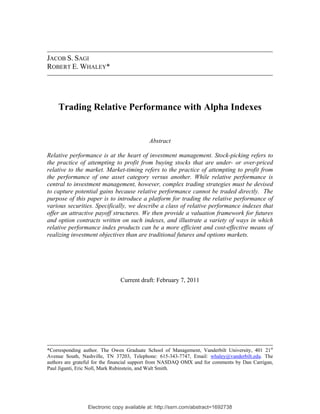
15. free bonds, illustrating that there is no limit to the loss that can be incurred from the short
benchmark-ETF position. On the other hand, the value of the fully collateralized alpha-
futures position is 25, well above its minimum level of 0.
Long stock-call, short benchmark-call: Oftentimes investors prefer to use
option-like structures in their trading strategies. To capture relative performance, an
investor could buy an at-the-money call option on the stock and sell an at-the-money call
option on the benchmark. Using the illustration above, the long stock-call would expire
worthless at the end of the investment horizon since the stock price, 50, sank below the
exercise price, 100. On other hand, the benchmark call is 100 dollars in the money at
expiration. Since the investor is short the call, he loses 100. As an alternative strategy, the
investor could choose to buy an at-the-money call on the alpha index (hereafter, “alpha-
call”). In the example, at the end of the call option’s life the index is at 25 and the call
expires worthless. Obviously, the alpha-call has less potential downside exposure.
To examine the potential upside of the alpha-call, we reverse the price movements
by letting the stock price go from 100 to 200 and the benchmark to go from 100 to 33.33.
The long stock-call/short benchmark-call strategy would have a payoff of 100 at
expiration because the stock-call is 100 in the money and the benchmark call is
worthless. On the other hand, the alpha index rises to a level of 600 leaving the alpha-call
500 in the money. Obviously, the alpha-call has greater upside potential.
Naturally, the decision about which strategy to use must be based on investor
preferences and other portfolio considerations. Our purpose is to illustrate how a static
position in an alpha-call differs from a position in existing instruments. To this end,
Figure 1 shows the value of the alpha-call as a function of the stock price and the
benchmark price at expiration. The call option has an exercise price of 100 and three
months remaining to expiration. The volatility rates of the stock (AAPL) and the
benchmark (SPY) are 26.7% and 17.9%, respectively. The correlation between the
returns is 0.711. The risk-free interest rate is 2%. Note that, as the stock price falls and
the benchmark price rises, the call goes to its lowest possible value of 0. On the other
hand, as the stock price rises, the call value rises, however, as the benchmark price falls,
14

16. the call value rises at an increasing rate. This is because the benchmark price is in the
denominator of the alpha index.
Figure 2 shows the value surface of the long stock-call/short benchmark-call
portfolio. The value of this portfolio position is scaled to match the value of the at-the-
money alpha-call option to ensure equal dollar investment. In general, the scale factor is
greater than one because the proceeds from the sale of the benchmark-call are used to
offset the purchase price of the stock-call. Like the alpha-call, the value of the long stock-
call/short benchmark-call portfolio falls in value as the stock price falls and/or the
benchmark price rises. Unlike the alpha-call, however, the portfolio value may become
negative. Moreover, as the stock price rises and the benchmark price falls, the portfolio
value rises, albeit not to the same levels as the alpha-call.
Long stock-call/long benchmark-put: Another option strategy that is designed
to capture relative performance is to buy an at-the-money stock-call and buy an at-the-
money benchmark-put. Returning to our illustration, suppose the stock price falls from
100 to 50 and the index level rises from 100 to 200. The long stock-call expires out of the
money, as does the long benchmark put. Hence, the “straddle” expires worthless, similar
to the alpha-call. If the reverse happens and the stock price rises to 200 and the
benchmark falls to 50, the stock-call is 100 in the money, the put is 50 in the money, and
the straddle value is 150. The alpha-call, on the other hand, has a value of 300.
Again, the decision about which strategy to use is based on investor preferences.
Figure 3 shows the value surface of the long stock-call/long benchmark-put portfolio at
expiration which can be compared with the corresponding alpha-call surface in Figure 1.
Here too the call-put position is scaled so that its initial value matches that of the alpha-
call. In general, the scale factor is less than one because two options are being purchased,
and the stock-call alone has a higher premium than the alpha-call. Like the alpha-call, the
value of the long stock-call/long benchmark-put portfolio falls in value as the stock price
falls and/or the benchmark price rises. And, also like the alpha-call, the call-put position
never falls below 0. On the other hand, as the stock price rises and the benchmark price
falls, the call-put position value does not rise to the same levels as the alpha-call.
15

17. To illustrate yet another important difference between the call-put strategy above
and the alpha-call, consider an unexpected change to market volatility. Roughly, the call-
put position value will be highly affected because both the call and the put are exposed to
market risk and move in the same direction in reaction to news about market volatility.
By contrast, the alpha-call value will be less affected for most stocks.17
The three strategy comparisons provided above illustrate the distinctive features
of alpha index derivatives. These products can simultaneously provide downside
protection while reducing exposure to market volatility. While existing exchange-traded
products can be combined to create a passive, directional bet on relative performance,
they cannot be combined to create a passive, directional bet on the alpha index or its
derivatives products. To do so would require dynamic trading strategies, and dynamic
strategies are prohibitively expensive, at least for retail investors.
To get a rough sense for the trading costs in replicating alpha-products, we
perform a set of simulations. In the simulations, the investor is assumed to pay a
proportional cost of $0.01 per share, a fixed cost of $1.00 for trading any quantity of the
stock, benchmark, or bond, and an additional 0.20% net fee for a short sale.18 The trading
strategy aims to replicate a $1,000 investment in a three-month, at-the-money alpha-call
option on the b = 1 AAPL vs. SPY index using standard delta-hedging techniques.19 The
volatility and correlation parameters are drawn from Table 2.
The simulation results are quite striking. In order to achieve a tracking standard
error no larger than about 5%, the average trading costs are around 110% of the value of
the position! The reason is that hedging an at-the-money call requires frequent
rebalancing (about 300 times during the three months to achieve the 5% standard tracking
error). Each time the portfolio is rebalanced the investor must pay $1 per trade, or $3 in
total to trade in risk-free bonds, AAPL, and SPY, amounting to about $900 over the life
of the option. The remaining $200 in average costs is generated by the proportional
17
In particular, if the stock’s beta is fixed at one then the alpha-call value only depends on the stock’s
idiosyncratic volatility.
18
We assume that the proportional costs for trading the short-term bond are negligible. Our cost
assumptions are conservative and understate the true trading costs currently faced by retail investors.
19
Specific details regarding the delta-hedge simulation are available from the authors upon request.
16

18. transaction costs and is still staggeringly large. In other words, even a $1M position in at-
the-money calls would require an expenditure of roughly 20% of the portfolio value in
trading costs if the standard tracking error is to be kept below 5%.
Table 3 documents simulation results of tracking errors and trading costs for
various three-month AAPL vs. SPY alpha-call options. The initial investment is assumed
to be $10,000, and the replicating portfolio is assumed to be rebalanced daily (90 trading
periods after the initial portfolio setup) over the life of the option. Note that the at-the-
money alpha-call now has a tracking error of 9% as opposed to the 5% in the earlier
illustration. This is because the replicating portfolio is rebalanced only 90 times as
opposed to 300. Out-of-the-money calls are the most difficult and costly to replicate. The
reason is that the high leverage implicit in such options requires large positions in the
stock and benchmark relative to the option value. Even small fluctuations in the
underlying prices can greatly unbalance the portfolio. In addition, the large trades
required for rebalancing entail higher costs. The 10% out-of-the-money alpha-call has an
average tracking error of 34% and an average total trading cost of 36% of the option’s
value. Overall, the lesson from this exercise is that, while forward/futures positions on an
alpha index might be relatively inexpensive to implement through dynamic trading,
replicating alpha-options is not.
B. Relative performance index options are generally less expensive
The fact that relative performance index products are less exposed to market risk
means that relative performance index options are less expensive than standard options.
The reason is simple. Stock options are based on the total risk of the stock (i.e., the sum
of market risk and idiosyncratic risk), while relative performance index options are
essentially based on the difference in risk between the stock and the benchmark. Because
option value varies directly with volatility, relative performance index options are
cheaper.
To illustrate, return once more to the AAPL vs. SPY example. Suppose an
investor decides to buy an at-the-money call option with an exercise price of 100 and
three months remaining to expiration. The investor estimates that the expected future
17

19. return volatility of AAPL is 26.7% and SPY is 17.9%, and that the expected correlation
between AAPL and SPY returns is 0.711. The risk-free interest is 2%. Under the BSM
assumptions, the value of an at-the-money call option on AAPL is $11.53. At the same
time, the value of an at-the-money call option on AVSPY is $7.24, corresponding to a
discount of 37%. The volatility used in the valuation of the relative performance index
option, given by equation (6), is 18.8%. As long as the correlation between the assets is
positive and σ S > σ M , the volatility of the index (i.e., σ ) is guaranteed to be smaller than
the volatility of the stock (i.e., σ S ), and the price an alpha-call will likewise be
guaranteed to be cheaper than the price on a target-call.
C. Relative performance index products are based on total return
Earlier, we argued that in order to make a fair comparison between the
performances of two securities, one should consider their total return, which includes
income distribution as well as price appreciation. There are other advantages to using
total returns in measuring performance. Standard exchange-traded stock futures and
option contracts are based only on the price appreciation of the underlying stock. Because
a relative performance index futures incorporates dividends into the performance
calculation, its payoffs implicitly include the automatic reinvestment of security income
without incurring transaction costs. It also means that relative performance index options
are not susceptible to the trading games played in the stock option market when deep in-
the-money options remain unexercised.20
D. Trading correlation
According to the valuation equations derived in Section II, the values of relative
performance index futures and options depend on the correlation between the security S
and the benchmark M. A higher correlation implies lower index futures and call options
prices. A trader who believes correlations will increase (decrease) can sell (buy) index
futures or sell (buy) index call options to benefit from his or her insights. With the earlier
20
Pool, Stoll, and Whaley (2008), for example, show that many long call option holders unwittingly fail to
exercise outstanding call option positions on stocks when it is optimal to do so (just prior to the ex-dividend
day) and, as a result, forfeit the ex-dividend call option price drop to market makers and proprietary firms.
18

20. example of AAPL vs. SPY, an increase in the correlation from 0.711 to 0.8 corresponds
to a decline in the value of a one-year at-the-money call option from $7.24 to $6.08. The
trader could sell the option and hope that the new information would be reflected in
prices soon after (at which point he or she would close out the position for a profit). The
risk here is that the index will simultaneously move higher, cancelling the decline in the
option value. To make a cleaner investment, the trader can hedge the written option using
the deltas calculated in Appendix B and using a correlation value of 0.711 to calculate the
hedging positions. The net position will be insensitive to changes in the index itself, but
once the new correlation value of 0.8 is absorbed by the market, the option value will
sink below that of the hedging portfolio and the trader can close out the portfolio at a
profit.21 The opposite strategy can be employed if the trader believes correlations will
decline. This illustrates how investors can trade on their views concerning correlations
between the index components.
In general, the construction of a portfolio that moves only with the correlation
between two assets requires model-calculated positions in relative performance index
derivatives and the index constituents (and potentially their derivatives). What is
important to emphasize is that such trades could not be contemplated without traded
index derivatives (just as one could not trade volatility without traded stock derivatives).
Thus, just as stock options have enabled markets to trade stock volatility, relative
performance index products have the potential of opening up an entirely new market for
trading correlations.
IV. Summary
The purpose of this paper is to introduce a new complex of relative performance
indexes, tracking the performance of a target security versus that of a benchmark
security. In particular, we assess how derivatives (options and futures) on these indexes
might provide investors with new opportunities to trade relative performance. We provide
21
This assumes that volatilities are constant. If this is not the case, then the trader would have to account
for changing volatility in constructing the hedging portfolio.
19

21. valuation formulae for futures and option contracts on the family of relative performance
indexes. In addition, we illustrate a variety of ways in which the new index products
could be a more efficient and cost-effective means of realizing certain investment
objectives than are traditional futures and options markets.
The new indexes essentially track a portfolio that is long on a target stock and
short on a benchmark asset, such that the ratio of the two dollar positions is constant. As
the target asset outperforms its benchmark, the equivalent long-short position increases.
Likewise, if the target asset underperforms its benchmark over a period, then the
equivalent portfolio long-short position is decreased. This behavior ensures downside
protection which could only otherwise be implemented through dynamic trading – an
exercise typically beyond the reach of most investors.
The introduction of options on the new indexes poses several additional benefits.
We show that such options are generally cheaper than options on the target security. We
also show that they offer a different payoff structure than related positions using standard
calls and puts on the underlying target and benchmark securities. In particular, the new
index call options simultaneously have downside protection and an accelerated upside
relative to static positions in existing instruments. At the same time, such options would
be creating investment opportunities otherwise only available to typical investors at great
costs. Finally, an exciting aspect of the new index options is that they present investors
with the ability to trade the correlation between the target and benchmark securities.
Indeed, we show that option implied correlations (which could be used to calculate option
implied target CAPM betas if the benchmark is a market index) are both forward-looking
and potentially more informative about future correlations than historical estimates.
20

22. References
Black, Fischer. 1976. The pricing of commodity contracts, Journal of Financial
Economics 3, 167-179.
Black, Fischer and Myron Scholes. 1973. The pricing of options and corporate liabilities,
Journal of Political Economy 81, 637-659.
Fischer, Stanley. 1978. Call option pricing when the exercise price is uncertain and the
valuation of index bonds, Journal of Finance 33, 169-176.
Margrabe, William. 1978. The value of an option to exchange one asset for another,
Journal of Finance 33, 177-186.
Merton, Robert C. 1973. Theory of rational option pricing, Bell Journal of Economics
and Management Science 1, 141-183.
Pool, Veronika, Hans R. Stoll, and Robert E. Whaley. 2008. Failure to exercise call
options: An anomaly and a trading game, Journal of Financial Markets 11, 1-35.
Reiner, Eric. 1992. Quanto mechanics, RISK 5, 59-63.
Rubinstein, Mark. 1991. One for another, RISK 4, 30-32.
Whaley, Robert E. 2006. Derivatives: Markets, Valuation, and Risk Management, John
Wiley & Sons, Inc.: Hoboken, New Jersey.
21

23. Appendix A: Multi-asset relative performance indexes
The benchmark used in the definition of the complex of relative performance
indexes in (1) can be extended to include multiple-asset benchmarks. Suppose, for
example, the desired benchmark has n different asset classes (i.e., stocks, bonds, real
estate, and commodities) and each asset class constitutes w% of the overall benchmark
n
portfolio, where, of course, ∑ w = 1 . Under these assumptions, the updating rule for the
i =1
i
multi-asset relative performance index is
I b , w,t +1 = I b , w,t ×
(1 + R )
S ,t +1
.
n
∏ (1 + R )
wi b
i ,t +1
i =1
where b is as before and w is a vector of benchmark asset allocation weights (i.e.,
wi , i = 1,..., n ) . With a relative performance so defined, a change in the log-index
corresponds to the difference between the instantaneous performance of security S versus
the weighted and scaled instantaneous performances of the benchmark assets, that is,
n
ln I b , w ,t +1 − ln I b , w ,t = ln (1 + RS ,t +1 ) − b ∑ wi ln (1 + Ri ,t +1 )
i =1
The futures and option valuation equations on these multi-factor benchmarks are also
analytically tractable and available from the authors upon request.
22

24. Appendix B: Risk metrics for derivatives on relative performance indexes
Under the BSM option valuation assumptions, we showed that the value of a
futures contract written on a relative performance index with a constant relative risk-
adjustment coefficient of b is
Fb = Ib e( r −δ )T , (B-1)
where Fb and Ib are the futures price and the relative performance index level, r is the
annualized risk-free interest rate, T is the futures time remaining to expiration in years,
bσ M
δ = br −
2
( (1 + b ) σ M − 2 ρ SM σ S ) , σ S and σ M are the volatility rates of the security
and the benchmark, and ρSM is the correlation between the returns of the security and the
benchmark. We also showed that the values of the European-style call and put options on
the relative performance index are
Cb = Ibe−δ T N ( d1 ) − Xe− rT N ( d2 ) , (B-2)
and
Pb = e− rT XN ( −d2 ) − Ibe−δ T N ( −d1 ) . (B-3)
where X is the exercise price of the option, T is the time remaining to option expiration
(i.e., same time as futures), N ( d ) is the cumulative normal density function with upper
integral limit d, σ = σ S + b2σ M − 2bρSM σ Sσ M , and the upper integral limits are
2 2
ln ( Ib / X ) + (r − δ + .5σ 2 )T
d1 = , and d 2 = d1 − σ T .
σ T
The put-call parity relation for European-style options is
Cb − Pb = Ib e−δ T − Xe− rT . (B-4)
Based on these equations, the risk metrics (i.e., delta, gamma and vega) of the futures and
options are as follows.
23

25. Delta: Based on the futures pricing relation (B-1), the delta of the futures with respect to
the underlying relative performance index is
Δ F , I = e( r −δ )T .
The deltas with respect to the prices of the security and the benchmark are
I b ( r −δ )T I r −δ T
Δ F ,S = e and Δ F , M = − b e( ) .
S M
Based upon the valuation equations (B-2) and (B-3), the deltas of the European-
style call and put options with respect to a change in the underlying relative performance
index are
Δc, I = e−δ T N ( d1 ) and Δ p, I = −e−δ T N ( −d1 ) .
Since the alpha options may be hedged using shares of the security or the benchmark, the
deltas with respect to the per share security price, S, are
Ib I
Δc,S = Δ c , I and Δ p , S = − b Δ p , I
S S
and the deltas with respect to the per share benchmark price, M, are
Ib I
Δc,M = − Δ c , I and Δ p , M = b Δ p , I .
M M
Gamma:
(B-5) shows that the delta is not a function of the relative performance index level, so the
gamma of a futures with respect to the index is 0. This is also true of the gamma with
respect to the security, S. The gamma with respect to the benchmark price is not zero,
however, and is given by
I b ( r −δ )T
Γ F , MM = 2 e .
M2
The cross gammas are
24

26. Ib
Γ F , SM = Γ F , MS = − Δ F ,I .
SM
The gamma of a call option with respect to the underlying index is the same as that for
the put option:
n ( d1 )
Γ I = Γ c , I = Γ p , I = e −δ T ,
I bσ T
1 − d12 / 2
where n ( d1 ) = e is the normal density function evaluated at d1 . The gammas of
2π
the call option with respect to the underlying security and benchmark prices are given by
I b2 I ( I Γ + 2Δ I ) I ( I Γ + ΔI )
Γ c,S = 2
Γ I , Γc,M = b b I 2 and Γ c , SM = Γ c , MS = − b b I .
S M SM
By virtue of the put-call parity relation (B-4), the gammas of the European-style put
options are related through the gamma of the futures price:
Γ p ,S = Γc ,S , Γ p,M = Γc,M − e− rT ΓF ,M and Γ p ,SM = Γ p,MS = Γc,MS − e− rT Γ F ,MS .
Vega:
Unlike the usual cost of carry model, the futures pricing equation for a relative
performance index is a function of volatility. The vegas with respect to σ S , σ M , and ρSM
are:
VegaF ,σ S = −b ρ SM σ M TFb ,
VegaF ,σ M = b ⎡(1 + b ) σ M − ρ SM σ S ⎤ TFb ,
⎣ ⎦
and
VegaF , ρSM = −bσ Sσ M TFb .
The vegas of the European-style call option with respect to σ S , σ M , and ρSM are
25

27. ⎛ σ − bρ SM σ M ⎞ − rT
Vegac ,σ S = I b e−δ T n ( d1 ) T ⎜ S ⎟ + e N ( d1 ) VegaF ,σ S
⎝ σ T ⎠
⎛ b ( bσ M − ρ SM σ S ) ⎞ − rT
Vegac ,σ M = I b e −δ T n ( d1 ) T ⎜ ⎟ + e N ( d1 ) VegaF ,σ M
⎝ σ T ⎠
and
⎛ bσ σ ⎞ − rT
Vegac , ρSM = − Ib e−δ T n ( d1 ) T ⎜ S M ⎟ + e N ( d1 ) VegaF , ρSM .
⎝ σ T ⎠
Note that, by the put-call parity relation (B-4), the vegas of the call, put and futures are
related by Vegac,i − Vega p,i = e− VegaF ,i , where i = σ S , σ M , ρSM . Hence, the vegas of the
rT
European-style put option with respect to σ S , σ M , and ρSM are
Vega p ,σ S = Vegac,σ S − e− rTVegaF ,σ S ,
Vega p ,σ M = Vegac,σ M − e− rTVegaF ,σ M ,
and
Vega p, ρSM = Vegac, ρSM − e− rTVegaF , ρSM .
26

28. Table 1: Simulation of replicating portfolio for the b = 1 relative performance index. At the beginning of each day, the
portfolio is rebalanced so that the position in cash and the target security is set equal to the level of the index, while the
portfolio position in the benchmark is short an amount equal to the level of the index. The table documents the daily income
from these positions, as well as the payout that results from rebalancing.
Relative Hedge portfolio Mimicking
Total return indexes performance index Interest Dollar income Net portfolio
Day Security Benchmark Level Gain income Security Benchmark gain Payout value
0 100 100 100 100
1 104.17 107.16 97.21 -2.79 0.070 4.170 7.160 -2.920 -0.130 97.21
2 108.61 111.53 97.38 0.17 0.068 4.143 3.964 0.247 0.075 97.38
3 110.68 110.36 100.29 2.91 0.068 1.856 -1.022 2.946 0.038 100.29
4 111.01 113.83 97.52 -2.77 0.070 0.299 3.153 -2.784 -0.017 97.52
5 112.62 110.70 101.73 4.21 0.068 1.414 -2.682 4.164 -0.048 101.73
27

29. Table 2: List of NASDAQ OMX Alpha Indexes™ with option contracts pending approval of the SEC. All of the indexes listed are
outperformance indexes with the benchmark being the SPDR ETF (ticker symbol SPY). The annualized volatility of each stock and
correlation with SPY are calculated using daily return data for the calendar year 2010. The data were collected from Datastream. Over the
sample period, SPY daily returns had a realized annualized volatility of 17.9%.
Alpha Stock return
Stock index Correlation
Stock name ticker ticker Volatility with SPY return
Amazon.com, Inc. AMZN ZVSPY 32.6% 60.4%
Apple Inc. AAPL AVSPY 26.7% 71.1%
Cisco Systems, Inc. CSCO CVSPY 31.9% 61.7%
Ford Motor Company F FVSPY 38.1% 70.6%
General Electric Company GE LVSPY 27.4% 82.3%
Google Inc. GOOG UVSPY 27.8% 65.1%
Hewlett Packard Company HPQ HVSPY 24.9% 68.0%
International Business Machines IBM IVSPY 17.8% 78.3%
Intel Corporation INTC JVSPY 25.3% 77.3%
Coca-Cola Company KO KVSPY 15.5% 63.7%
Merck & Company, Inc. MRK NVSPY 20.6% 65.7%
Microsoft Corporation MSFT MVSPY 22.0% 73.0%
Oracle Corporation ORCL OVSPY 24.4% 67.5%
Pfizer Inc. PFE PVSPY 21.3% 66.2%
Research in Motion Limited RIMM RVSPY 38.5% 44.9%
AT&T Inc. T YVSPY 15.1% 70.7%
Target Corporation TGT XVSPY 20.2% 66.0%
Verizon Communications Inc. VZ VVSPY 16.0% 60.3%
Wal-Mart Stores, Inc. WMT WVSPY 14.0% 50.3%
28

30. Table 3: Transaction costs and tracking error for delta-hedging portfolios of positions in three-month futures and options positions
written on the AVSPY alpha index. Following the initial setup, the hedging portfolio is rebalanced 90 times in equal intervals (“days”)
subsequent to the initial investment of $10,000. Fixed costs are set at $1 per asset per trade. Proportional costs are set to $0.01 per share, with
initial share values for AAPL and SPY taken to be $340 and $130, respectively. Short selling costs are assumed to be 0.20% of the amount
borrowed. The AAPL volatility rate is assumed to be 26.7%, the SPY volatility rate is 17.9%, and the correlation between the two returns is
71.1%. The index is set to 100 when the derivative positions are initiated. The table reports the standard deviation of the tracking error,
defined as the difference between the option value and the value of the tracking portfolio at expiry in the absence of transaction costs. The
table also reports a breakdown of the accrued trading costs at the option’s expiration. The fixed costs can accrue to more than $273 because
costs are capitalized. They can also be below that value for deep out-of-the-money options because certain price paths lead to essentially zero
option value well before the option’s expiration.
Tracking Average fixed Average proportional Average total
Derivative standard error (%) costs ($) costs ($) costs (%)
Futures 0.1% $274 $30 3%
Call option
X=80 0.5% $274 $160 4%
X=90 2% $274 $400 7%
X=100 9% $272 $1,300 16%
X=110 34% $268 $3,300 36%
29

31. F
Figure 1: Simul lated expiration value of call op ption on AVSPY index. The ca option has an exercise price o 100 and three months
Y all of
r
remaining to exppiration. The vol
latility rates of th security (AAPL) and the ben
he nchmark (SPY) a 26.7% and 1
are 17.9%, respective The
ely.
c
correlation betwe the returns is 0.711. The risk-fr interest rate is 2%.
een 0 free s
200
150
100
Option value
50
0
-50
-100
50
50
70
60
70
90
80
90
100
110
110
120
130
130
140
Benchmark price
B 150 Security price
30

32. F
Figure 2: Simulaated expiration value of portfolio consisting of lo call option o AAPL and sho call option on SPY. Both call options
v o ong on ort l
h
have an exercise price of 100 and three months rem
maining to expiraation. The volatili rates of the se
ity ecurity (AAPL) a the benchmar (SPY)
and rk
a 26.7% and 17
are 7.9%, respectivel The correlatio between the re
ly. on eturns is 0.711. T risk-free inte
The erest rate is 2%. P
Portfolio value o at-the-
of
m
money options at origination is sca to match the value of the at-th
aled he-money alpha c option.
call
200
150
100
Option value
50
0
-50
-100
50
50
70
60
70
-150
90
80
90
100
110
110
120
130
130
140
150
Be
enchmark price Security price
31

33. F
Figure 3: Simulaated expiration value of portfolio consisting of lo call option o AAPL and lo put option on SPY. Both call and put
v ong on ong n l
o onths remaining to expiration. The volatility rates o the security (AA
options have an exercise price of 100 and three mo
e 1 o of APL) and the ben
nchmark
(
(SPY) are 26.7% and 17.9%, respectively. The cor rrelation between the returns is 0.7
711. The risk-free interest rate is 2 Portfolio valu of at-
e 2%. ue
t
the-money option at origination is scaled to match the value of the at-the-money alp call option.
ns h pha
200
150
100
Option value
50
0
-50
-100
50
50
70
60
70
90
80
90
100
110
110
120
130
130
140
150
Be
enchmark price Security price
32