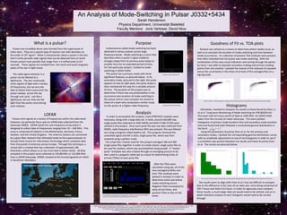
1. An Analysis of Mode-Switching in Pulsar J0332+5434
Sarah Henderson
Physics Department, Universität Bielefeld
Faculty Mentors: Joris Verbiest, David Nice
Pulsars are incredibly dense stars formed from the supernovae of
other stars. They are a special type of neutron star with densities on
the order of 1017 kg/m3. What is characteristic about a pulsar is the fact
that it emits periodic radio signals that can be detected here on Earth.
Known pulsars have periods that range from 1.4 milliseconds to 8.5
seconds. These signals are emitted from the north and south magnetic
poles of the star in light cones.
The radio signal emission in a
pulsar can be likened to a
lighthouse. The star continually
emits signals of light with a variety
of frequencies, but we are only
able to detect them every time the
pulsar sweeps across the sky
through one cycle. Just like a
lighthouse, we can only see the
light from the pulsar once during
each rotation.
“Long-term Monitoring of Mode Switching for PSR B0329+54.” Chen, J. L. et al. The Astrophysical Journal, Volume 741, Issue 1. Nov. 2011. IOP. <http://adsabs.harvard.edu/abs/2011ApJ...741...48C>.
“Pulsar Properties.” National Radio Astronomy Observatory. Associated Universities Inc., 12 Nov. 2009. Web. 7 Sept. 2015. <http://www.cv.nrao.edu/course/astr534/Pulsars.html>.
“The LOFAR Telescope.” ASTRON: Netherlands Institute for Radio Astronomy. 2015. Web. 7 Sept. 2015. <https://www.astron.nl/lofar-telescope/lofar-telescope>.
“The PSRCHIVE Project.” PSRCHIVE. Willem van Straten, 2006-2013. Web. 7 Sept. 2015. <http://psrchive.sourceforge.net/>.
van Straten, W; Demorest, P & Oslowski, S. 2012. Astronomical Research and Technology 9: 237.
http://www.jamiewieck.com/wp-content/uploads/2010/01/pulsar.jpg
LOFAR
Pulsars emit signals at a variety of frequencies within the radio band.
However, my particular focus was on LOFAR data collected from the
telescope DE605. LOFAR stands for Low Frequency Array which is
designed to collect data at frequencies ranging from 10 – 240 MHz. This
array is comprised of stations in the Netherlands, Germany, France,
Sweden, and the United Kingdom. The antenna stations are connected
by a glass fiber network that ultimately leads to the supercomputer at
Donald Smits Centre for Information Technology which combines data
from thousands of antennas across Europe. Through this technique, a
virtual dish is created that has a diameter of approximately 100
kilometers, which allows us to see more data in better detail. All data
analyzed in this project were collected at 139.88 MHz or 153.809 MHz
from a LOFAR telescope, DE605, located at the Forschungszentrum Jülich
in Nordrhein Westfalen.
A phenomena called mode-switching has been
observed in various pulsars across large
frequency bands. Mode-switching is a term that
describes when a pulsar’s signal suddenly
changes shape from its primary pulse shape to
another form for an extended period of time.
For this particular project, I looked at mode-
switching in J0332+5434.
This pulsar has a primary mode with three
significant features, as pictured above. In its
secondary mode, pictured to the right, the pulse
appears to lose its right peak; the pulse shape is
then maintained this way for a variable amount
of time. The purpose of this project was to
determine if there was any predictability in the
occurrence and duration of mode-switching in
this pulsar and to cross compare my results to
those of a team who conducted a similar study
on this pulsar at a higher radio frequency.
Primary mode for J0332+5434
Purpose
Secondary mode for J0332+5434
In order to accomplish this analysis, many PSRCHIVE modules were
necessary, along with a large data set. In total, around 540,000 raw,
single-pulse files collected on MJD 56550 and MJD 57160-57164 were
utilized in this project. Since each pulse file was raw data collected from
DE605, radio frequency interference (RFI) was present; this was filtered
out using a program called Zapthis.csh. This program removed the
unwanted signal and left a clear, single-pulse file, which was then
analyzed using a python script.
The script that I mainly used for this project averaged 100 and 300
single-pulse files together in order to create clearer, single-pulse files to
be used for analysis, which was accomplished using psradd. A “master
pulse” template was also created through an averaging process to be
later used in a program called pat as a basis for determining times of
arrivals (TOAs) of each pulse file.
https://www.astron.nl/sites/astron.nl/files/cms/PDF/LOFAR%20international%20stations%20on%20map%20Europe.jpg
Analysis
After the TOAs were
calculated using pat, all of the
new averaged profiles and
their TOA residuals were
plotted in tempo2 in order to
determine when and where
mode-switching occurs.
Negative TOAs correspond to
early arrival times, and
positive TOAs to late arrival
times.An example of a tempo2 plot for 100 pulse files. Modes can be seen on this tempo2
plot as the columns of points corresponding to late arrival times.
Goodness of Fit vs. TOA plots
Tempo2 was utilized as a means to determine where modes occur, as
well as to calculate the duration of mode-switching and time between
mode occurrences. If a collection of positive TOA residuals were present,
that often indicated that the pulsar was mode-switching. With the
combination of this easy visual indication and sorting through the points
by hand, I was able to separate secondary moding and primary moding
points from one another. I plotted the inverse of the reduced chi squared
versus the uncertainty in the times of arrivals of the averaged files on a
log-log scale.
Plots of 1/GOF vs. TOA uncertainty on a log-log scale for all 100 pulse files analyzed (left) and 300 pulse files analyzed (right).
Histograms
Ultimately, I wanted to compare my results to those found by Chen J.L.
et al in “Long-term Monitoring of Mode Switching for PSR B0329+54.”
This team had 521 hours worth of data at 1540 MHz for J0332+5434
taken from the Urumqi 25 meter telescope. This team plotted
histograms of primary mode duration time and secondary mode duration
time and found that both followed a constrained gamma distribution in
the form:
Using the parameters found by Chen et al. for the primary and
secondary modes, I plotted the corresponding gamma distribution curves
with an amplitude adjustment on top of my histograms in order to see if
a correlation was present between my results and those found by Chen
et al. The results are pictured below.
My results seem to align with Chen et al.’s but are difficult to compare
due to the difference in the sizes of our data sets, mine being comprised of
105.7 hours and theirs 512 hours. In order to rigorously cross compare
these results, a much larger data set would need to be utilized, and an in-
depth statistical analysis of each histogram would need to be carried
through.
Primary mode durations (green) and secondary mode durations (blue) plotted with corresponding constrained gamma distributions.
What is a pulsar?