SlideShare una empresa de Scribd logo
1 de 33
Chapter 1
Copulas, Sklar’s Theorem, and Distributional
Transform


In this chapter we introduce some useful tools in order to construct and analyse
multivariate distributions. The distributional transform and its inverse the quantile
transform allow to deal with general one-dimensional distributions in a similar
way as with continuous distributions. A nice and simple application is a short
proof of the general Sklar Theorem. We also introduce multivariate extensions,
the multivariate distributional transform, and its inverse, the multivariate quantile
transform. These extensions are a useful tool for the construction of a random vector
with given distribution function respectively allow to build functional models of
classes of processes. They are also a basic tool for the simulation of multivariate
distributions. We also describe some applications to stochastic ordering, to goodness
of fit tests and to a general version of the empirical copula process. We introduce
to some common classes of copula models and explain the pair copula construction
method as well as a construction method based on projections. In the final part
extensions to generalized Fr´ chet classes with given overlapping multivariate
                               e
marginals are discussed. The construction of dependence models by projections is
extended to the generalized Fr´ chet class where some higher dimensional marginals
                               e
are specified.


1.1 Sklar’s Theorem and the Distributional Transform

The notion of copula was introduced in Sklar (1959) to decompose an n-dimensional
distribution function F into two parts, the marginal distribution functions Fi and the
copula C , describing the dependence part of the distribution.
Definition 1.1 (Copula). Let X D .X1 ; : : : ; Xn / be a random vector with distribu-
tion function F and with marginal distribution functions Fi , Xi Fi , 1 Ä i Ä n. A
distribution function C with uniform marginals on Œ0; 1 is called a “copula” of X if

                                   F D C.F1 ; : : : ; Fn /:                           (1.1)

L. R¨ schendorf, Mathematical Risk Analysis, Springer Series in Operations Research
    u                                                                                    3
and Financial Engineering, DOI 10.1007/978-3-642-33590-7 1,
© Springer-Verlag Berlin Heidelberg 2013
4                                       1 Copulas, Sklar’s Theorem, and Distributional Transform


  By definition the set of copulas is identical to the Fr´ chet class F .U; : : : ; U/ of all
                                                        e
distribution functions C with uniform marginals distribution functions

                                      U.t/ D t;      t 2 Œ0; 1:                          (1.2)

For the case that the marginal distribution functions of F are continuous it is easy
to describe a corresponding copula. Define C to be the distribution function of
.F1 .X1 /; : : : ; Fn .Xn //. Since Fi .Xi / U.0; 1/ have uniform distribution C is a
copula and furthermore we obtain the representation

                 C.u1 ; : : : ; un / D P .F1 .X1 / Ä u1 ; : : : ; Fn .Xn / Ä un /
                                   D P .X1 Ä F1 1 .u1 /; : : : ; Xn Ä Fn 1 .un //
                                   D FX .F1 1 .u1 /; : : : ; Fn 1 .un //:                 (1.3)

          1
Here Fi        denotes the generalized inverse of Fi , the “quantile transform”, de-
fined by

                             Fi 1 .t/ D inffx 2 R1 I Fi .x/           tg:

C is a copula of F since by definition of C

              F .x1 ; : : : ; xn / D P .X1 Ä x1 ; : : : ; Xn Ä xn /
                               D P .F1 .X1 / Ä F1 .x1 /; : : : ; Fn .Xn / Ä Fn .xn //
                               D C.F1 .x1 /; : : : ; Fn .xn //:                           (1.4)

    The argument for the construction of the copula is based on the property that
for continuous distribution functions Fi , Fi .Xi / is uniformly distributed on .0; 1/:
Fi .Xi / U.0; 1/. There is a simple extension of this transformation which we call
“distributional transform.”
Definition 1.2 (Distributional transform). Let Y be a real random variable with
distribution function F and let V be a random variable independent of Y , such that
V      U.0; 1/, i.e. V is uniformly distributed on .0; 1/. The modified distribution
function F .x; λ/ is defined by

                            F .x; λ/ WD P .X < x/ C λP .Y D x/:                           (1.5)

We call

                                          U WD F .Y; V /                                  (1.6)

the (generalized) “distributional transform” of Y .
1.1 Sklar’s Theorem and the Distributional Transform                                       5


      For continuous distribution functions F , F .x; λ/ D F .x/ for all λ, and U D
          d             d
F .Y / D U.0; 1/, D denoting equality in distribution. This property is easily ex-
tended to the generalized distributional transform (see e.g. R¨ 1 (2005)).
                                                              u
Proposition 1.3 (Distributional transform). Let U D F .Y; V / be the distribu-
tional transform of Y as defined in (1.6). Then

                                       d
                                   U D U.0; 1/ and Y D F             1
                                                                         .U / a.s.      (1.7)

      An equivalent way to introduce the distributional transform is given by

                                  U D F .Y / C V .F .Y /              F .Y //;          (1.8)

where F .y / denotes the left-hand limit. Thus at any jump point of the distribution
function F one uses V to randomize the jump height.
   The distributional transform is a useful tool which allows in many respects to deal
with general (discontinuous) distributions similar as with continuous distributions.
In particular it implies a simple proof of Sklar’s Theorem in the general case (see
Moore and Spruill (1975) and R¨ (1981b, 2005)).
                                 u
Theorem 1.4 (Sklar’s Theorem). Let F 2 F .F1 ; : : : ; Fn / be an n-dimensional
distribution function with marginals F1 ; : : : ; Fn . Then there exists a copula C 2
F .U; : : : ; U/ with uniform marginals such that

                                F .x1 ; : : : ; xn / D C.F1 .x1 /; : : : ; Fn .xn //:   (1.9)

Proof. Let X D .X1 ; : : : ; Xn / be a random vector on a probability space
. ; A; P / with distribution function F and let V    U.0; 1/ be independent of X .
Considering the distributional transforms Ui WD Fi .Xi ; V /, 1 Ä i Ä n, we have by
                            d
Proposition 1.3 Ui D U.0; 1/ and Xi D Fi 1 .Ui / a.s., 1 Ä i Ä n. Thus defining C
to be the distribution function of U D .U1 ; : : : ; Un / we obtain

              F .x/ D P .X Ä x/ D P .Fi 1 .Ui / Ä xi ; 1 Ä i Ä n/
                     D P .Ui Ä Fi .xi /; 1 Ä i Ä n/ D C.F1 .x1 /; : : : ; Fn .xn //;

i.e. C is a copula of F .
Remark 1.5. (a) Copula and dependence. From the construction of the distri-
   butional transform it is clear that the distributional transform is not unique
   in the case when the distribution has discrete parts. Different choices of the


1
    Within the whole book the author’s name is abbreviated to R¨ .
                                                               u
6                                                1 Copulas, Sklar’s Theorem, and Distributional Transform

Figure 1.1 Copula of                                                    1
uniform distribution on line
segments (published in: Journal of Stat.
Planning Inf., 139: 3921–3927, 2009)


                                                                        1
                                                                        2


                                                                                        1               1
                                                                                        2


    randomizations V at the jumps or in the components, i.e. choosing Ui D
    Fi .Xi ; Vi /, may introduce artificial local dependence between the components
    of a random vector on the level of the copula. From the copula alone one does
    not see whether some local positive or negative dependence is a real one or
    just comes from the choice of the copula. For dimension n D 2 the copula in
    Figure 1.1 could mean a real switch of local positive and negative dependence
    for the original distribution, but it might also be an artefact resulting from the
    randomization in case the marginals are e.g. both two-point distributions while
    the joint distribution in this case could be even comonotone. Thus the copula
    information alone is not sufficient to decide all dependence properties.
(b) Conditional value at risk. A more recent application of the distributional trans-
    form is to risk measures. It is well known that the conditional tail expectation

                                              TCE˛ .X / WD   E.X j X Ä q˛ /;                      (1.10)

        where q˛ is the lower ˛-quantile of the risk X , does not define a coherent risk
        measure except when restricted to continuous distributions. This defect can be
        overcome by using the distributional transform U D F .X; V / and defining the
        modified version, which we call conditional value at risk (CVR˛ )

                                              CVR˛ .X / D E.X j U Ä ˛/:                           (1.11)

        By some simple calculations (see Burgert and R¨ (2006b)) one sees that
                                                      u

                                           1
              CVR˛ .X / D                    EX1.X < q˛ / C q˛ ˛       P .X < q˛ /     D ES˛ .X /:
                                           ˛
                                                                                                  (1.12)

        Thus the more natural definition of CVR˛ coincides with the well-established
        “expected shortfall risk measure” ES˛ .X / which is a coherent risk measure.
1.2 Copula Models and Copula Constructions                                             7


    As a consequence the expected shortfall is represented as conditional expec-
    tation and our definition in (1.11) of the conditional value at risk seems to be
    appropriate for this purpose.
(c) Stochastic ordering. The construction of copulas based on the distributional
    transform as in the proof of Sklar’s Theorem above has been used in early papers
    on stochastic ordering. The following typical example of this type of result is
    from R¨ (1981b, Proposition 7).
            u
    Proposition 1.6. Let Fi , Gi be one-dimensional distribution functions with
    Fi Ä Gi (or equivalently Gi Äst Fi ), 1 Ä i Ä n. Then to any F 2F .F1 ; : : : ; Fn /
    there exists an element G 2 F .G1 ; : : : ; Gn / with G Äst F . Here Äst denotes the
    multivariate stochastic ordering w.r.t. increasing functions.
    Proof. Let X D .X1 ; : : : ; Xn / F and let Ui D Fi .Xi ; V / denote the distri-
    butional transforms of the components Xi . Then U D .U1 ; : : : ; Un / is a copula
    vector of F . Define Y D .Y1 ; : : : ; Yn / as vector of the quantile transforms of
    the components of U , Yi D Gi 1 .Ui /. Then Y            G 2 F .G1 ; : : : ; Gn / and
    from the assumption Fi Ä Gi we obtain that Y Ä X pointwise. In consequence
    G Äst F .
    In particular the above argument shows that G Äst F if F and G have the same
    copula.                                                                    ˙


1.2 Copula Models and Copula Constructions

In order to construct a distributional model for a random vector X it is by Sklar’s
representation theorem sufficient to specify a copula model fitting to the normalized
data. There are a large number of suggestions and principles for the construction of
copula models. Classical books on these models for n D 2 are Mardia (1962) and
Hutchinson and Lai (1990). More recent books for n        2 are Joe (1997), Nelsen
(2006), Mari and Kotz (2001), Denuit et al. (2005), and McNeil et al. (2005b).
A lot of material on copulas can also be found in the conference volumes of the
“Probability with given marginals” conferences – i.e. the series of conferences in
Rome (1990), Seattle (1993), Prague (1996), Barcelona (2000), Qu´ bec (2004),
                                                                       e
Tartu (2007) and Sao Paulo (2010) as well as in the recent proceedings edited
by Jaworski, Durante, H¨ rdle, and Rychlik (2010). A huge basket of models has
                          a
been developed and some of its properties have been investigated, concerning in
particular the following questions:
• What is the “range of dependence” covered by these models and measured with
  some dependence index. Is the range of dependence wide and flexible enough?
• What models exhibit tail dependence and thus are able to model situations with
  strong positive dependence in tails?
• Is some parameter available describing the degree of dependence?
8                                      1 Copulas, Sklar’s Theorem, and Distributional Transform


• Is there a natural probabilistic representation respectively interpretation of these
  models describing situations when to apply them?
• Is there a closed form of the copula or a simple simulation algorithm so that
  goodness of fit test can be applied to evaluate whether they fit the data?
Several questions of this type have been discussed in the nice survey papers of
Schweizer (1991) and Durante and Sempi (2010).


1.2.1 Some Classes of Copulas

Copulas, their properties and applications are discussed in detail in the above-
mentioned literature. Copulas are not for any class of distributions the suitable
standardizations as for example for elliptical distributions. In extreme value theory
a standardization by the exponential distribution may be better adapted. For some
applications it may be more natural and simpler to model the distributions or
their densities directly without referring to copulas. Conceptually and for some
investigation of dependence properties like tail-dependence the notion of copula
is however a useful tool.
    Some classical classes of copulas are the following.
• The “Farlie–Gumbel–Morgenstern (FGM) copula”:

                      C˛ .u; v/ D uv.1 C ˛.1            u/.1        v//;   j˛j Ä 1       (1.13)

    as well as its generalized versions, “EFGM copulas” are extensions of FGM to
    the n-dimensional case and given by
                                                                                     !
                               Q
                               n                   X                Q
                   C.u/ D             ui 1 C                   ˛T   j 2T .1   uj /       (1.14)
                               i D1
                                               T   f1;:::;ng


  for suitable ˛T 2 R1 .
• The “Archimedean copulas”

                      Cˆ .u1 ; : : : ; un / D ˆ 1 .ˆ.u1 / C             C ˆ.un //        (1.15)

    for some generator ˆ W .0; 1 ! RC with ˆ.1/ D 0 such that ˆ is com-
    pletely monotone. In fact Cˆ is an n-dimensional copula if and only if ˆ is
    “n-monotone”, i.e. ˆ is .n 2/ times differentiable and

                       . 1/k ˆ.k/ .t/       0;     0ÄkÄn                2; 8t > 0        (1.16)

    and . 1/n 2 ˆ.n   2/
                           is decreasing and convex (see McNeil and Neˇlehov´ (2010)).
                                                                      s     a
1.2 Copula Models and Copula Constructions                                                    9


      In case ˆ.t/ D ˛ .t
                     1         ˛
                                   1/ one gets the “Clayton copula”

                                    X                       Á   1=˛
                      C˛ .u/ D           ui   ˛
                                                      nC1             ;   ˛ > 0:          (1.17)

   In case ˆı .t/ D   1
                      ı
                          log.1     .1    e ı /e t / one gets the “Frank copula”
                                          Â    Qn       ıui    Ã
                                     1          i D1 .e     1/
                      Cı .u/ D         log 1 C                   :                        (1.18)
                                     ı          .e ı 1/n 1

   ˆ is by Bernstein’s theorem completely monotone if and only if it is n-monotone
   for all n 2 N.
      Archimedean copulas are connected with mixing models (“frailty models”).
   Let                             Z Y n
                          FX .x/ D       .Gi .xi //ı dF‰ .ı/;
                                              i D1

   where ‰ is a positive real mixing variable. Then with L‰ , the Laplace transform
   of ‰, we obtain that the i -th marginal is given by
                           Z
              Fi .xi / D        exp.ı ln Gi .xi //dF‰ .ı/ D L‰ . ln Gi .xi //:

   As a consequence one gets
                                              ÂX
                                               n                      Ã
                               FX .x/ D L‰                  1
                                                         L‰ .Fi .xi // ;                  (1.19)
                                                  i D1

   i.e. a representation as in (1.15) holds with the generator ˆ D L‰ which by
   Bernstein’s theorem is completely monotone.
       Archimedean copulas arise from multivariate distributions that have a stochas-
   tic representation of the form
                                                  d
                                          X DR U                                          (1.20)
          U
  whereP is uniformly distributed on the unit simplex (1-sphere) in            fx 2Rn ,
                                                                                    C
           n
  Rn I
    C      i D1 xi D 1g respectively the simplex in Rn , and R is a scaling random
  variable with values in RC independent of U . Formulae for the relation between
  the distribution function FR and the generator ˆ are available (see McNeil and
  Neˇlehov´ (2010)).
     s       a
• “Elliptical distributions” arise from stochastic representations of the form

                                         XD           C RAU;                              (1.21)

   where U is uniformly distributed on the unit 2-sphere Sn 1 D fx 2 Rn ;
   Pn
     i D1 ui D 1g in R . R is a real positive random variable independent from
           2          n

   U and A is an n n-matrix. X has a density of the form
10                                1 Copulas, Sklar’s Theorem, and Distributional Transform


                f .x/ D j†j 1 ˆ..x            /> † 1 .x             // with † D AA> :

     The distribution is denoted as E. ; †; FR /. Multivariate normal distributions
  are elliptical (or elliptically contoured). The copulas of elliptical distributions are
  in general not available in closed form.
• “Extreme value copulas” are defined as possible limits of max sequences. Let
  Xi D .Xi;1 ; : : : ; Xi;d /, 1 Ä i Ä n (note that here d D dimension but n D
  sample index) be a sequence of iid random vectors with copula CF . Let Mn D
  maxfX1 ; : : : ; Xn g D .Mn;1 ; : : : ; Mn;d / be the componentwise max of the Xi ,
  then the copula Cn of Mn is given by
                                                      n     1=n      1=n
                              Cn .u/ D CF .u1 ; : : : ; ud /:

       C is called an “extreme value copula” if for any n 2 N there exist some
     copula CF such that
                                              n           1=n      1=n
                                C D CF .u1 ; : : : ; ud /:                              (1.22)

     A well-known fact is:
     C is an extreme value copula if and only if C is “max stable”, i.e. C.u/ D
       m 1=m          1=m
     C .u1 ; : : : ; ud / for all m 2 N.
        De Haan and Resnick (1977) and Pickands (1981) gave the following
     representation of extreme value copulas:
     C is an extreme value copula if and only if it has a representation of the form

                        C.u/ D exp. l. log u1 ; : : : ;                  log ud //:     (1.23)

     Here the “tail dependence function” l W .0; 1/d ! Œ0; 1 is given by
                                     Z
                            l.x/ D                    max.wj xj /dH.w/                  (1.24)
                                         Sd       1
                                                      j Äd

                                                            R
     where H is a measure on the simple Sd 1 satisfying Sd 1 wj dH.w/ D 1,
     1 Ä j Ä d . H is called the “spectral measure” of C .
        An example of copulas which are of interest in extreme value theory are
     “Gumbel copulas” given by
                                         Â                 X
                                                           n             Á1=ı Ã
                        Cı .u/ D exp                         . log ui /ı                (1.25)
                                                           i D1


     for ı 2 Œ1; 1/. Gumbel copulas are extreme value copulas. The parameter ı is a
     dependence parameter. If 1 Ä ı1 < ı2 , then Gı2 is more strongly dependent (in
     the sense of supermodular ordering) than Gı1 (see Wei and Hu (2002)).
1.2 Copula Models and Copula Constructions                                                   11


1.2.2 Copulas and L2 -Projections

A general principle for the construction of dependence models (copulas) was
introduced in R¨ (1985). It is based on the following representation result. Let
                  u
Cn .λ n / denote the set of all copulas on Œ0; 1n which are Lebesgue-continuous and
     n
thus have Lebesgue-densities f . Let Cn .λ n / be the set of all signed measures on
                                            s n
      n
Œ0; 1 with uniform marginals and which have Lebesgue-densities f .
    For any integrable f 2 L1 .Œ0; 1n ; λ n / and T
                                          n            f1; : : : ; ng we define
                                        Z
                                                 Q
                                 fT D        f       i 2T   dyi ;                         (1.26)

i.e. we integrate over the components in T . We consider fT as a real function
on Œ0; 1n being constant in the T components. The following linear operator
S W L1 .λ n / ! L1 .λ n / is of interest,
         n           n

                                     X
                      Sf D f                     fT C .n            1/ff1;:::;ng          (1.27)
                                  T f1;:::;ng
                                   jT jDn 1


since it leads to the following representation result.
Theorem 1.7 (Copulas and L2 -projections). All probability distributions on
Œ0; 1n with Lebesgue-density and uniform marginals are of the form .1 C Sf /λ n
                                                                              n
where f 2 L1 .λ n /, more precisely
                n

                              ˚                                 «
                   Cn .λ n / D Q D .1 C Sf /λ n I f 2 L1 .λ n /
                    s n                      n             n                              (1.28)

and                      ˚                                                           «
              Cn .λ n / D P D .1 C Sf /λ n I f 2 L1 .λ /; Sf
                   n                    n             n                             1 :   (1.29)
Proof. Any P 2 Cn .λ n / has by the Radon–Nikod´ m theorem a density of the
                         s n
                                                       y
form P D .1 C f /λ n where fT D 0 for jT j n 1. This implies that Sf D f ,
                           n
i.e. P D .1 C Sf /λ n . Conversely, let f 2 L1 .λ n / and P D .1 C Sf /λ n . Then for
                         n                         n                          n
T0     f1; : : : ; ng, jT0 j D n 1 and any further T    f1; : : : ; ng with jT j D n 1,
T 6D T0 we have .fT /T0 D ff1;:::;ng and, therefore,
                 Â                  X                                        Ã
        .Sf /T0 D f        fT0               fT C .n          1/ff1;:::;ng                (1.30)
                                  jT jDn 1                                     T0
                                    T 6DT0
                                   X
                 D fT0    fT0               .fT /T0 C .n             1/ff1;:::;ng D 0:    (1.31)
                                 jT jDn 1
                                   T 6DT0
12                                        1 Copulas, Sklar’s Theorem, and Distributional Transform


Therefore Q D .1 C Sf /λ n 2 Cn .λ n /. This implies (1.28). Equation (1.29) is
                        n     s n

immediate from (1.28).
   The operator S in (1.27) can be considered as an L2 -projection of a (signed)
measure Q D .1 C f /λ n , f 2 L1 .λ 1 / to a copula P D .1 C Sf /λ n if Sf
                         n             n                             n            1.
The basic idea of the construction method for dependence (copula) models in R¨     u
(1985) is to describe in a first step the relevant dependence by the density function
1 C f . In a second step this model Q D .1 C f /λ n is projected to the class of
                                                       n
copulas in the form P D .1 C Sf /λ n .n
   The resulting proposed model construction method is the following:
Construction by “projection method”: Let f# , # 2 ‚ be a parametric family
of functions in L1 .λ n / (describing the intended dependence structure) such that
                     n
Sf#      1, # 2 ‚. Then the proposed model obtained by the projection method is
given by                      ˚                          «
                        P D P# D .1 C Sf# /λ n I # 2 ‚ :
                                                n                           (1.32)
   The inherent idea in this construction is the hope that the projection on the correct
marginal structure does not change the intended dependence structure too much.
Obviously we can use the same procedure as above also for the construction of
elements in the Fr´ chet class M.P1 ; : : : ; Pn / which are continuous w.r.t. a product
                       e
measure 1 ˝ ˝ n .
   This projection idea is also underlying Sklar’s representation theorem. Let G 2
Fn .G1 ; : : : ; Gn / be a multivariate distribution function with marginals G1 ; : : : ; Gn
and with copula C . Assume that G is a good description of the dependence
structure for a model. At the same time assume that the correct marginals should
be F1 ; : : : ; Fn instead of G1 ; : : : ; Gn . Then by Sklar’s Theorem the following
“nonmetric projection” would seem natural:

                                 G ! C ! F D C.F1 ; : : : ; Fn /:                          (1.33)

By this transition the dependence structure is retained in the copula C . The difficulty
of calculation may however prevent use of this transition in examples. Typically it
will be easier to calculate (only) densities.
   The following examples illustrate the projection method, see R¨ (1985) and Mari
                                                                    u
and Kotz (2001, pp. 73–78).
                                                 ˚                        «
Example 1.8. Let f 2 L1 .λ n /, let ˛0 D inf .Sf /.x/I x 2 Œ0; 1n > 1 and
                               n

consider f# .x/ D #f .x/, # 2 Œ0; j˛0 j .
                                     1

                                                Q                   R
(1) Generalized FGM-family: If f .x/ D nD1 vi .xi / where vi .xi /dxi D 0,
                                                   i
     1 Ä i Ä n, then Sf D f and P gives a “generalized FGM-family” (see
     Johnson and Kotz (1975) and KimeldorfQ Sampson (1975a,b), and (1.13)).
                                                and
(2) Polynomial copula models: If f .x/ D nD1 ximi is a polynomial, then
                                                 i
                                                          !
                   Q
                   n               X
                                   n
                                            Q        1                       Q
                                                                             n       1
        Sf .x/ D          ximi                              ximi C .n   1/                 (1.34)
                   i D1            i D1    j 6Di   mj C 1                    i D1 mi C 1
1.2 Copula Models and Copula Constructions                                                         13


    gives a “polynomial copula model” which is the same as the FGM-model
    generated by vi .xi / D ximi mi1 . Linear combinations then yield the general
                                    C1
    form of polynomial copula models. The restrictions to the parameters are given
    in Mari and Kotz (2001, p. 74).
        This polynomial model has also been discussed in Wei, Fang, and Fang
    (1998). Several families of polynomial copulas have been suggested as local
    approximations of other copula families. So the Ali–Mikhail–Haq family is a
    polynomial approximate in the neighbourhood of the independence copula, the
    FGM is an approximation of the Plackett family (see Mari and Kotz (2001,
    p. 75)).
(3) A copula concentrated strongly near the diagonal: Let n D 2 and consider
    f .x; y/ D p 1 . The function f has singularities at the diagonal, i.e. we
                     jx yj
    expect a large density in the neighbourhood of the diagonal. Then by simple
    calculation one gets

                     1                 p  p                   p  p              Á 8
      Sf .x; y/ D p                2    xC 1             xC    yC 1            y C : (1.35)
                   jx yj                                                          3

       P describes a family of copulas which is concentrated near the diagonal. # is
    a positive dependence parameter; higher values of # yield higher order positive
    dependence.
(4) Diagonal weakly concentrated copula: For ‚ D Œ0; 1, n D 2 define

                                   f# .x; y/ D       1fjx   yj>#g ;


    so .1 C f# /λ 2 is concentrated in a neighbourhood of the diagonal but it is
                 n
    uniformly distributed on f.x; y/ 2 Œ0; 12 W jx yj Ä #g in contrast to the
    singular concentration in Example 1.8, (1.8).
       By the projection to the correct marginals we obtain

                 Sf# .x; y/ D f# .x; y/ C g# .x/ C g# .y/                .1    #/2 ;         (1.36)

    where

       g# .x/ D .2      2#/1f#ÄxÄ1     #g   C .1     x      y/1.0Äx<#/        .x   y/1.x>1    #/

                               1
                 for 0 Ä # Ä
                               2

    and g# .x/ D .x #/1.x>#/ C .# x/1.x<1 #/ , 1 < # Ä 1.
                                                     2
       The projected probability model P# D .1 C Sf# /λ 2 approaches for # ! 1
                                                        n
    the product measure while for # small (neglecting small and large x-values)
                                             (
                                                 2   2#     for jx    yj < #;
                     1 C .Sf# /.x; y/                                                        (1.37)
                                                 1   2#     for jx    yj > #:
14                                     1 Copulas, Sklar’s Theorem, and Distributional Transform


     In order to introduce a stronger dependence effect one can start with f#;a .x; y/
     D af# .x; y/ which for # small and a large centres the distribution near the
     diagonal.                                                                      ˙


1.3 Multivariate Distributional and Quantile Transform

The distributional transform F .X; V / as well as the inverse quantile transform
F 1 .V / have been generalized to the multivariate case.
Definition 1.9 (Multivariate quantile transform).               Let F be a d -dimensional
distribution function and let V1 ; : : : ; Vn be iid U.0; 1/-distributed random variables.
Then the “multivariate quantile transform” Y WD F 1 .V / is defined recursively as

                 Y1 WD F1 1 .V1 /
                                                                                          (1.38)
                 Yk WD Fkj1;:::;k 1 .Vk j Y1 ; : : : ; Yk 1 /;
                          1
                                                                   2 Ä k Ä n;

where Fkj1;:::;k 1 denote the conditional distribution functions of the k-th component
 k given the first k    1 components 1 ; : : : ; k 1 .
   The multivariate quantile transform is a basic method to construct a random vec-
tor Y with specified distribution function F from a given vector V D .V1 ; : : : ; Vn /
of iid uniformly on Œ0; 1 distributed random variables. By construction the mul-
tivariate quantile transform uses only one-dimensional conditional distribution
functions.
Theorem 1.10 (Multivariate quantile transform).         The multivariate quantile
transform Y D F 1 .V / is a random vector with distribution function F .
Proof. In case n D 2 and for any x1 ; x2 2 R we have using the independence of
.Vi /
                                   Z    x1
      P .Y1 Ä x1 ; Y2 Ä x2 / D               P .Y2 Ä x2 j Y1 D y1 /dF1 .y1 /
                                        1
                                   Z    x1
                               D             P .F2j11 .V2 j y1 / Ä x2 j Y1 D y1 /dF1 .y1 /
                                        1
                                   Z    x1
                               D             P .F2j11 .V2 j y1 / Ä x2 /dF1 .y1 /
                                        1
                                   Z    x1
                               D             F2j1 .x2 j y1 /dF1 .y1 / D F12 .x1 ; x2 /:
                                        1

   By induction this argument extends to yield P .Y1 Ä x1 ; : : : ; Yn Ä xn / D
F .x1 ; : : : ; xn /.
1.3 Multivariate Distributional and Quantile Transform                                                15


   The multivariate quantile transform was introduced in O’Brien (1975), Arjas and
Lehtonen (1978), and R¨ (1981b). The construction Y is an inductive construction
                       u
of a random vector with specified distribution function F and is called “regression
representation” since Y is of the form

                                      Y1 D h1 .V1 /;
                                      Y2 D h2 .Y1 ; V2 /;
                                      Y3 D h2 .Y1 ; Y2 ; V3 /;                                     (1.39)
                                         :
                                         :
                                         :
                                      Yn D hn .Y1 ; : : : ; Yn 1 ; Vn /

representing Yk as function of the past Y1 ; : : : ; Yk 1 and some innovation Vk . As a
consequence this implies the “standard representation”

                             Yk D fk .V1 ; : : : ; Vk /;      1 Ä k Ä n:                           (1.40)

   The multivariate quantile transform and particularly Theorem 1.10 is a basic
method for the “simulation of multivariate distributions”. In order to construct
a random vector with distribution function F one needs to simulate iid U.0; 1/-
random variables and to determine the inverses of the one-dimensional conditional
distribution functions Fi jx1 ;:::;xi 1 .xi /, which can be done in many examples either
analytically or numerically. There is a large literature on (Monte Carlo) simulation
of multivariate distributions, which uses essentially the multivariate quantile trans-
form. This transform was introduced first in the above-mentioned papers dealing
with representation of stochastic sequences and with stochastic orderings.
Definition 1.11 (Multivariate distributional transform).                     Let X be an n-
dimensional random vector and let V1 ; : : : ; Vn be iid U.0; 1/-distributed random
variables, V D .V1 ; : : : ; Vn /. For λ D .λ1 ; : : : ; λn / 2 Œ0; 1n define

   F .x; λ/   WD F1 .x1 ; λ1 /; F2 .x2 ; λ2 j x1 /; : : : ; Fd .xd ; λd j x1 ; : : : ; xd   1/   ; (1.41)

where

                          F1 .x1 ; λ1 / D P .X1 < x1 / C λ1 P .X1 D x1 /;
      Fk .xk ; λk j x1 ; : : : ; xk    1/   D P .Xk < xk j Xj D xj ; j Ä k            1/
                                                C λk P .Xk D xk j Xj D xj ; j Ä k                1/

are the distributional transforms of the one-dimensional conditional distributions.
Finally the “multivariate distributional transform”of X is defined as

                                             U WD    F .X; V /:                                    (1.42)
16                                    1 Copulas, Sklar’s Theorem, and Distributional Transform


   Rosenblatt (1952) introduced this transformation in the special case of absolutely
continuous conditional distributions allowing the application of the transformation
formula. Therefore this transformation is also called the “Rosenblatt transforma-
tion” in this case. For general distributions the multivariate distributional transform
(generalized Rosenblatt transform) was introduced in R¨ (1981b). The basic
                                                               u
property is stated in the following theorem in R¨ (1981b).
                                                  u
Theorem 1.12 (Multivariate distributional transform). Let X be a random vec-
tor and let U D F .X; V / denote its multivariate distributional transform. Then

(a)                                           U    U..0; 1/d /;                                 (1.43)
         i.e. the components Ui of U are iid U.0; 1/ distributed.
                                                           1
(b) The multivariate quantile transform                F       is inverse to the multivariate distribu-
    tional transform, i.e.

                            XD        F
                                          1
                                              .U / D       F
                                                               1
                                                                   .   F .X; V //   a.s.        (1.44)

Proof. U1 D F1 .X1 ; V1 / U.0; 1/ by Proposition 1.3. Consider next U2 D F2 .X2 ;
V2 j X1 /. Conditionally given X1 D x1 we have again from Proposition 1.3 that

                                d
                           U2 D F2 .X2 ; V2 j x1 /                      U.0; 1/:

Furthermore, P U2 jX1 Dx1 D U.0; 1/ is independent of x1 and thus U2 , X1 are
independent. Since U1 D F1 .X1 ; V1 / we get from iterated conditional expectation
that also U2 , U1 are independent. The general case then follows by induction.

Remark 1.13 (Regression and standard representation).
(a) By combining the multivariate quantile and the multivariate distributional trans-
    form one gets for any given stochastic sequence .Xk / a pointwise “standard
    (innovation) representation”

                                    Xk D fk .U1 ; : : : ; Uk / a.s.;                            (1.45)

      respectively a pointwise “regression representation”

                      Xk D fk .X1 ; : : : ; Xk 1 ; Uk / a.s.;                  1ÄkÄn            (1.46)

      with some iid sequences .Ui /, Ui      U.0; 1/. This result was proved first for
      n D 2 in Skorohod (1976). Related functional representations of classes of
      stochastic models are given in R¨ and de Valk (1993). For example in the case of
                                      u
      Markov chains the regression representation reduces to the following functional
      representation of (any) Markov chain:
      Corollary 1.14 (Regression representation of Markov chains). Any Markov
      chain .Xn / has a representation as a nonlinear regression model
1.4 Pair Copula Construction of Copula Models                                                  17


                                  Xk D fk .Xk 1 ; Uk / a.s.;                                (1.47)

    where .Uk / is an iid sequence of U.0; 1/-distributed random variables, Uk is
    independent of X1 ; : : : ; Xk 1 .
(b) The copula transformation

               X D .X1 ; : : : ; Xd / ! U D .U1 ; : : : ; Ud /; Ui D Fi .Xi ; Vi /

    which transforms a vector X to a copula vector U , where U corresponds to
    the copula of X , forgets about the marginals but retains essential information
    on the dependence structure of X . On the contrary the multivariate distribu-
    tional transform forgets also about the dependence structure. This is an interest-
    ing property, when one wants to identify a distribution. These two different
    properties of the copula transformation and the multivariate distributional
    transform lead to different kinds of applications. Some of them are described in
    Section 1.5.                                                                    ˙


1.4 Pair Copula Construction of Copula Models

Besides the multivariate quantile transform in Theorem 1.10, which is based on
the one-dimensional conditional distributions Fi jx1 ;:::;xi 1 , several further methods
to represent a distribution function F in terms of conditional distribution functions
have been proposed. Particular interest in the recent literature and in various
applications arose from the “pair copula construction (PCC)” method which is
based on a series of certain (organized) pairs of variables.
   In the original example Joe (1997) used the following pairwise construction of an
m-dimensional distribution function F . For m D 3, F D F123 can be represented as
                                     Z   x2
                        F123 .x/ D            F13jz2 .x1 ; x3 /dF2 .z2 /                    (1.48)
                                         1

where F13jz2 is the conditional distribution function of the pair X1 ; X3 given X2 D z2 .
By Sklar’s Theorem this can also be written in terms of the conditional copula C13jz2
in the form
                            Z x2
                 F123 .x/ D       C13jz2 .F1jz2 .x1 /; F3jz2 .x3 //dF2 .z2 /:     (1.49)
                                1

Similarly for general m one obtains recursively the representation
                Z x2     Z xm 1
   F1:::m .x/ D      :::        C1mjz2 ;:::;zm 1 F1jz2 ;:::;zm 1 .x1 /;
                   1        1                                                               (1.50)
                                     Fmjz2 ;:::;zm 1 .xm / dF2:::m 1 .z2 ; : : : ; zm 1 /

which is given in terms of pairwise conditional copulas.
18                                             1 Copulas, Sklar’s Theorem, and Distributional Transform


   In Bedford and Cooke (2001, 2002) and Kurowicka and Cooke (2006) some
general classes of graphical organization principles representing multivariate distri-
butions were developed. See also the survey of Czado (2010). Two basic examples
of these classes of constructions are C -vines and D-vines (C D canonical, D D
drawable).
(a) D-vines: The construction of D-vines is based on densities and uses the
    representation

                                                           Y
                                                           n
                                  f .x1 ; : : : ; xn / D          fi jx1 ;:::;xi 1 .xi /f1 .x1 /:                             (1.51)
                                                           i D2

     By Sklar’s Theorem we have

                             f12 .x1 ; x2 / D c12 .F1 .x1 /; F2 .x2 //f1 .x1 /f2 .x2 /;                                       (1.52)

     where c12 is a bivariate copula density. This implies for the conditional density

                                    f1jx2 .x1 / D c12 .F1 .x1 /; F2 .x2 //f1 .x1 /:                                           (1.53)

     Using (1.53) for the conditional density of .X1 ; Xi / given X2 ; : : : ; Xi                                              1   we
     obtain by recursion

                       fi jx1 ;:::;xi 1 .xi / D c1;i j2;:::;i       1   fi jx2 ;:::;xi 1 .xi /
                                                                                    !
                                                       Y
                                                       i 2
                                                D             cj;i jj C1;:::;i     1    ci     1;i       fi .xi /             (1.54)
                                                       j D1


     using the conditional copula densities

          cj;i jj C1;:::;i    1   D cj;i jxj C1 ;:::;xi 1 .Fj jxj C1 ;:::;xi 1 .xj /; Fi jxj C1 ;:::;xi 1 .xi //:

     As a result we obtain the “D-vine” density decomposition
                                                                                   !
                                                YY
                                                n i 2                                  Y
                                                                                       n                     Y
                                                                                                             n
                f .x1 ; : : : ; xn / D                      cj i jj C1;:::;i   1              ci       1;i         fl .xl /
                                                i D2 j D1                              i D2                  lD1

                                                n 1Y
                                                                                                   !
                                                Yn i                                                   Y
                                                                                                       n
                                         D                  cj;i Cj j.j C1;:::;j Ci           1/              fl .xl /:       (1.55)
                                                i D1 j D1                                              lD1


     The conditional copula densities in (1.55) are evaluated at the conditional
     distribution functions Fj jxj C1 ;:::;xj Ci 1 ; Fi Cj jxj C1 ;:::;xj Ci 1 .
1.4 Pair Copula Construction of Copula Models                                                                        19


     § ¤                   § ¤                  § ¤                         § ¤                      § ¤
      1                      2                    3                         4                          5        T1
     ¦ ¥  ¨¦ ¥  ¨¦ ¥  ¨¦ ¥  ¨¦ ¥
                 12                    23                    34                           45                    T2
                ©
                                  ¨ ©
                                                        ¨ ©
                                                                                  ¨ ©
                                                                                    
                          13 j 2                24 j 3                  35 j 4                                  T3
                                  ©
                                             
                                              ¨          ©
                                                                     
                                                                      ¨             ©
                                    14 j 23               25 j 34                                               T4
                                            ©                       ©
                                                         ¨
                                              15 j 234                                                          T5
                                                          ©
Figure 1.2 D-vine tree for n D 5


        The D-vine decomposition in (1.55) can be organized iteratively by pairwise
    copulas using iteratively levels T1 ; : : : ; Tn 1 . For n D 5 we obtain the represen-
    tation

          f .x1 ; : : : ; x5 /
                Y
                5
            D         fl .xl /c12 c23 c34 c45 c13j2 c24j3 c35j4 c14j23 c25j34 c15j234 :
                lD1


    This is described in the following graphical organization. Each transition step
    from level Ti to level Ti C1 involves a (conditional) pair copula (Figure 1.2).
(b) C -vines: C -vine decompositions are obtained when applying the representa-
    tion of the conditional density successively to the conditional distribution of
    Xi 1 ; Xi given X1 ; : : : ; Xi 2 . This gives

                            fi jx1 ;:::;xi 1 .xi / D ci   1;i jx1 ;:::;xi   2
                                                                                fi jx1 ;:::;xi 1 .xi /:         (1.56)

    Using (1.56) instead of (1.54) in (1.51) we obtain the C -vine decomposition

                                                          YY
                                                          n i 1
                      f .x1 ; : : : ; xn / D f1 .x1 /                 ci     k;i j1;:::;i k 1 fk .xi /
                                                          i D2 kD1
                                                                                          !
                                                  Yk 1
                                                  n Y                                          Y
                                                                                               n
                                            D                 ci   k;i j1;:::;i k 1                  fk .xk /
                                                  i D2 kD1                                     kD1
                                                                                          !
                                                  YY
                                                  n 1n j                                      Y
                                                                                              n
                                            D                 cj;j Ci j1;:::;j        1             fk .xk /:   (1.57)
                                                  j D1 i D1                                   kD1
20                                          1 Copulas, Sklar’s Theorem, and Distributional Transform


                         § ¤
                                                                                           ¨
                      ¦ ¥ 2
                  12                                                         j 1 ©
                                § ¤                                               13
                  
          § ¤ ((( 3 (( 3                                             ¨  23        ¨
               ( 1
               (                ¦ ¥                                       25 j 1
     T1 :  1 `                                                  T2 :
          ¦ ¥ ``5 ``
                   1                                                  12              15
               Z 1 `                                                  © 24 j
                                                                         b            ©
                 Z4           ``` § ¤                                     b 1  ¨
                                     ` 5                                     b
                  Z                    ¦ ¥                                      b 14
                     Z       § ¤                                                           ©
                        Z 4
                             ¦ ¥
                                     ¨
                      j12  25 j 1
                          
                ¨
                   35                 ©                                           ¨                        ¨
                                                                                   45 j 123
          23 j 1 a 34 j                                                  34 j 12                35 j 12
                 ©aaa
     T3 :                                                       T4 :
                       12                                                        ©                        ©
                         aa          ¨
                               24 j 1
                                     ©
Figure 1.3 C -vine for n D 5


      For n D 5 (1.57) gives a decomposition of the form

                                   Y
                                   5
          f .x1 ; : : : ; x5 / D         fk .xk /c12 c13 c14 c15 c23j1 c24j1 c25j1 c34j12 c35j12 c45j123 ;
                                   kD1

      which is represented by the following graph in Figure 1.3 with levels T1 ; : : : ; T4 .
      Again each transition of level Ti to Ti C1 involves (conditional) pair copulas.
Remark 1.15. (a) PCC and Markov random fields:
    More general systems to organize pairwise conditional copulas in order to
    represent uniquely an n-dimensional distribution function respectively density
    are described in Bedford and Cooke (2001, 2002) and Kurowicka and Cooke
    (2006) under the denomination “regular vine”. These decompositions are
    represented graphically as a nested tree. Edges of the tree denote the indices
    used in the conditional copula densities. The representation of the density in
    terms of these conditional distributions is an analogue of the Hammersley–
    Clifford theorem for Markov random field specifications by certain conditional
    distributions (of the components given their neighbourhoods). Depending on
    the choice of the neighbourhoods there is some strong similarity between both
    ways of constructing multivariate (spatial) models.
(b) Reduction of vine representation:
    Haff, Aas, and Frigessi (2010) consider a reduction of the (great) complexity
    of regular vine models by assuming that the conditional copula densities
    cj;i Cj jj C1;:::;j Ci 1 respectively copulas C1j j2;:::;j 1 do not depend on the var-
    iables xk in the condition but they depend only through the conditional
    distribution functions Fj jxj C1 ;:::;xj Ci 1 etc. This reduction seems to yield good
    approximations in several applications.                                             ˙
1.5 Applications of the Distributional Transform                                                                   21


1.5 Applications of the Distributional Transform

1.5.1 Application to Stochastic Ordering

Let Äst denote the usual stochastic ordering on Rn , i.e. the integral induced ordering
w.r.t. the class Fi of increasing functions which is defined by

                      X Äst Y if Ef .X / Ä Ef .Y / for all f 2 Fi                                              (1.58)

such that the expectations exist.
   The following sufficient condition for the multitivariate stochastic order is a
direct consequence of Theorem 1.10 on the multivariate quantile transform.
Proposition 1.16. Let X , Y be n-dimensional vectors with distribution functions
F , G 2 Fn and let .Vi /1Äi Än be iid, U.0; 1/-distributed, then

                            F
                                1
                                    .V / Ä   G
                                                 1
                                                     .V / implies that X Äst Y:                                (1.59)

   Condition (1.59) is stated in R¨ (1981b). It implies various sufficient conditions
                                  u
for stochastic ordering going back to classical results of Veinott (1965), Kalmykov
(1962), and Stoyan (1972). The comparison result of Veinott (1965) states
Corollary 1.17 (Comparison w.r.t. stochastic order Äst ). Let X , Y be n-dimen-
sional random vectors such that X1 Äst Y1 and for 2 Ä i Ä n

                    P Xi jX1 Dx1 ;:::;Xi     1 Dxi     1
                                                           Äst P Yi jY1 Dy1 ;:::;Yi    1 Dyi   1
                                                                                                               (1.60)

for all xj Ä yj , 1 Ä j Ä i             1, then

                                                      X Äst Y:

Proof. Condition (1.60) implies (by induction) that                          F
                                                                                 1
                                                                                     .V / Ä    G
                                                                                                   1
                                                                                                       .V / where F D
                                       d                             d
FX , G D FY . Since     F
                            1
                                .V / D X and            G
                                                            1
                                                                .V / D Y this implies X Äst Y .
   The standard construction in (1.45) respectively the regression representation
in (1.46) however are not applicable in general when P Äst Q, i.e. they do not in
general produce pointwise a.s. constructions X       P, Y      Q such that X Ä Y
a.s. The existence of such a coupling is however true under general conditions as
follows from the following theorem due to Strassen (1965).
   Let .S; Ä/ be a Polish space supplied with a closed semiorder “Ä”, i.e., the set
f.x; y/ 2 S S I x Ä yg is closed w.r.t. the product topology. The closed order Ä
induces the “stochastic order” Äst on the set M 1 .S / of probability measures on S
defined by
22                                     1 Copulas, Sklar’s Theorem, and Distributional Transform

                     Z             Z
      P Äst Q if         f dP Ä        f dQ
                                                                                                      (1.61)
          for all integrable increasing real functions f 2 Fi D Fi .S; Ä/:

Theorem 1.18 (Strassen’s ordering theorem, Strassen (1965)).
Let .S; Ä/ be a Polish space supplied with a closed partial order. Let P; Q 2
M 1 .S /, then

     P Äst Q
         , There exist random variables X                   P; Y       Q such that X Ä Y a.s.

   In Section 3.4 we will discuss extensions of this a.s. ordering theorem to the
class of “integral induced orderings ÄF ” for some function class F . These are
defined via
                        Z          Z
             P ÄF Q if     f dP Ä f dQ for all integrable f 2 F :

Early sources for integral induced orderings are Marshall and Olkin (1979), R¨    u
(1979), and Whitt (1986).
   The regression and standard constructions are used essentially in various papers
and textbooks on stochastic ordering and are closely connected with some notions
of stochastic ordering respectively dependence orderings. We state as one example
the notion of conditional increasing in sequence (CIS).
Definition 1.19 (Conditional increasing in sequence (CIS)).
A random vector X D .X1 ; : : : ; Xn / is called “conditional increasing in sequence”
(CIS)if for 2 Ä i Ä n
                              Xi st .X1 ; : : : ; Xi 1 /;                      (1.62)
i.e. the conditional distribution Pi jx1 ;:::;xi   1
                                                       D P Xi jX1 Dx1 ;:::;Xi   1 Dxi   1   is stochastically
increasing in .x1 ; : : : ; xi 1 /.
    The CIS-property of a random vector X is a positive dependence property of X .
This property is equivalent to the condition that the standard representation based
on the multivariate quantile transform Y D F 1 .V / is an increasing function in V ,
i.e.
             Yk D fk .V1 ; : : : ; Vk / are increasing in V; 2 Ä k Ä n:       (1.63)
Proposition 1.20 (CIS and multivariate quantile transform).
Let X be a random vector with distribution function F , then X is CIS if and only
if the construction by the multivariate quantile transformation Y D F 1 .V / D
.f1 .V1 /; f2 .V1 ; V2 /; : : : ; fn .V1 ; : : : ; Vn // is monotonically increasing in V .
1.5 Applications of the Distributional Transform                                                                  23


1.5.2 Optimal Couplings

The multivariate quantile transform is by Theorems 1.10 and 1.12 a basic con-
struction method for random vectors. An extension of this construction leads to
interesting connections with the construction of (optimal) couplings of distributions.
   Let h W Rn ! Rm be a measurable function and let P 2 M 1 .Rn ; Bn / have
distribution function F . Let furthermore S , V be random variables on . ; A; R/
such that the “distributional equation”

                                                   P h D RS ;

holds, i.e. h and S have the same distributions w.r.t. P respectively R.
Theorem 1.21 (Solution of stochastic equations, Ru (1985) and Rachev and Ru
                                                    ¨                            ¨
(1991)). Let S be a random variable on a probability space . ; A; R/ that satisfies
the distributional equation
                                  P h D RS :
Assume that V D .Vi /1Äi Än are further iid U.0; 1/-distributed random variables on
. ; A; R/ such that S , V are independent. Then there exists a random variable X
on . ; A; R/ such that
(a) RX D P , i.e. X has distribution function F
and
(b) X is a solution of the “stochastic equation”

                                       h ı X D S a.s. with respect to R:

Remark 1.22. The situation is described by the following diagram:
                                      S
                    . ; A; R/                      .Rm ; Bm /
                                                        
                                                       
                                         X           
                                                    
                                                    h
                                                  
                                                 
                                 .Rn ; Bn ; P / 

   If the distributional equation RS D P h holds, then there exists a solution X
with RX D P solving the stochastic equation h ı X D S a.s. and thus making the
diagram commutative.                                                           ˙
Proof. We denote by

                                                                          i j 1 Dx1 ;:::; i   1 Dxi
         Fi jx1 ;:::;xi   1 ;s
                                 D Fi . j x1 ; : : : ; xi   1 ; s/   DP                               1 ;hDs


the conditional distribution function of the i -th projection i given                                 j   D xj , j Ä
i 1 and given h D s and define inductively a random vector X by
24                                       1 Copulas, Sklar’s Theorem, and Distributional Transform


                   X1 D F1 1 .V1 j S /;           X2 D F2 1 .V2 j X1 ; S /; : : : ;
                                                                                                               (1.64)
                   Xn D Fn 1 .Vn j X1 ; : : : ; Xn 1 ; S /:

Equation (1.64) is an extension of the multivariate quantile transform. By the
independence assumptions we obtain

                RX1 jS Ds D RF1
                                      1 .V jS /jS Ds                     1 .V jS Ds/
                                                                                            1 jhDs
                                          1
                                                           D R F1            1
                                                                                       DP            :

Similarly,
                                                       1
                     RX2 jX1 Dx1 ;S Ds D RF2               .V2 jX1 ;S /jX1 Dx1 ;S Ds

                                                       1
                                                           .V2 jx1 ;s/           2 j 1 Dx1 ;hDs
                                          D R F2                         DP

implying
                                 Z
             R.X1 ;X2 /jS Ds D       RX2 jX1 Dx1 ;S Ds dRX1 jS Ds
                                 Z
                                          2 j 1 Dx1 ;hDs             1 jhDs
                           D         P                        dP              .x2 / D P .    1 ; 2 /jhDs
                                                                                                           :


By induction we find RX jS Ds D P jhDs and, therefore, RX D P .
   Since almost surely w.r.t. P h it holds that P jhDs .fxI h.x/ D sg/ D 1 we obtain
  X jS Ds
R         .fxI h.x/ D sg/ D 1ŒRS  and thus
                                      Z
             R.fh.X / D S g/ D             RX jS Ds .fxI h.x/ D sg/dRS .x/ D 1:

Remark 1.23. Using a measure isomorphism argument Theorem 1.21 on the
solutions of stochastic equations extends to Borel spaces E, F , replacing Rn , Rm
                                                                                        h                       f
(see R¨ (1985) and Rachev and R¨ (1991)), i.e. let .E; P / ! F , and . ; R/ ! F
      u                            u
be functions such that the distributional equation

                                               P h D Rf                                                        (1.65)

holds. If .E; P / is rich enough, i.e. it allows a uniformly U.0; 1/-distributed random
variable V on .E; P / independent of h, then there exists a random variable X W
E ! F with P X D R such that X solves the stochastic equation

                                           h D f ı X ŒP :                                                     (1.66)

                                                                                                                    ˙
1.5 Applications of the Distributional Transform                                           25


  An interesting application of Theorem 1.21 is to the construction of optimal
couplings. Let T W .Rn ; Bn / ! .Rm ; Bm / and for probability measures P; Q 2
M1 .Rn ; Bn / define the optimal coupling problem:
                             n                                                   o
                                                                       d      d
             cT .P; Q/ WD inf EkT .X /                    T .Y /k2 I X D P; Y D Q :     (1.67)

Equation (1.67) is the optimal coupling of T .X /, T .Y / over all possible couplings
X , Y of P , Q. Then the following result holds (see R¨ (1986)):
                                                       u
Corollary 1.24 (Optimal coupling of T ). Let P1 D P T , Q1 D QT be the distri-
butions of T under P , Q. Then
                    n                                            o
                                                       d      d
     cT .P; Q/ D inf EkT .X /             T .Y /k2 I X D P; Q D Q D `2 .P1 ; Q1 /;
                                                                     2


where `2 .P1 ; Q1 / is the “minimal `2 -metric” of P1 ; Q1 given by
                                n                                                  o
                                                                      d        d
             `2 .P1 ; Q1 / D inf .EkU                   V k2 /1=2 I U D P1 ; V D Q1 :   (1.68)

   In case m D 1 it holds that
                                          Z       1
                      `2 .P1 ; Q1 /
                       2              D               .F1 1 .u/   G1 1 .u//2 d u;       (1.69)
                                              0

where F1 ; G1 are the distribution functions of P1 ; Q1 .


1.5.3 Identification and Goodness of Fit Tests

For the construction of a goodness of fit test for the hypothesis H0 W F D F0
the multivariate distributional transform allows to construct simple test statistics by
checking whether the transformed random vectors Yi D F0 .Xi ; V i /, 1 Ä i Ä n,
are uniformly distributed on the unit cube Œ0; 1d . Standard tests for this purpose
                                                                      b
are based on Kolmogorov–Smirnov test statistics Tm D supt 2Œ0;1 jF m .t/ tj on
                                R
                                   b          2
Cram´ r–von Mises statistics .F m .t/ t/ dt or on weighted variants of them.
      e
                                        b
Here m D d n is the sample size and F m the corresponding empirical distribution
function. A detailed discussion of this principle and its practical and theoretical
properties is given in Prakasa Rao (1987). A main problem for the practical
application of this construction method is the calculation of conditional distribution
functions.
   This principle of standardization is also useful for various other kinds of
identification problems and for statistical tests as for example for the test of the
two-sample problem H0 W F D G. For this problem we use the empirical version of
26                                 1 Copulas, Sklar’s Theorem, and Distributional Transform


the distributional transform based on the pooled sample. We have to check whether
the transformed sample is a realization of a U.Œ0; 1d /-distributed variety.


1.5.4 Empirical Copula Process and Empirical Dependence
      Function

We consider the problem of testing or describing dependence properties of multi-
variate distributions based on a sequence of observations. The construction of test
statistics is typically based on some classical dependence measures like Kendall’s
or Spearman’s % (see Nelsen (2006)) or related dependence functionals. Empirical
versions of the dependence functionals can often be represented as functionals of
the reduced empirical process, the empirical copula function and the normalized
empirical copula process. The distributional transform allows to extend some limit
theorems known for the case of continuous distributions to more general distribution
classes.
   Let Xj D .Xj;1 ; : : : ; Xj;k /, 1 Ä j Ä n be k-dimensional random vectors with
distribution function F 2 F .F1 ; : : : ; Fk /. For the statistical analysis of dependence
properties of F a useful tool is the “reduced empirical process”, which is also called
“copula process”, and is defined for t 2 Œ0; 1k by

                         1 X
                               n
              Vn .t/ WD p        I Uj;1 Ä t1 ; : : : ; Uj;k Ä tk     C.t/ :          (1.70)
                          n j D1

Here Uj D .Uj;1 ; : : : ; Uj;k / are the copula vectors of Xj , Uj;i D Fi .Xj;i ; V j /, and
C is the corresponding copula C.t/ D P .Uj Ä t/.
   The construction of the distributional transforms Uj;i is based on knowing the
marginal distribution functions Fi . If Fi are not known it is natural to use empirical
versions of them. Let

                                        1X
                                            n
                            b
                            F i .xi / D        1.   1;xi  .Xj;i /                   (1.71)
                                        n j D1

denote the empirical distribution functions of the i -th components of X1 , : : : , Xn .
Then in the case of a continuous distribution function F the empirical counterparts
of the distributional transforms are
                                                                    Á
                    b        b           b      b              b
                   U j;i WD F i .Xj;i /; U j D U j;1 ; : : : ; U j;k :          (1.72)

For continuous distribution function Fi we have that

                                b        b
                               nU j;i D nF i .Xj;i / D Rj;i
                                                        n
                                                                                     (1.73)
1.5 Applications of the Distributional Transform                                                  27


are the ranks of Xj;i in the n-tuple of i -th components X1;i ; : : : ; Xn;i of X1 ; : : : ;
Xn and the ranks R1;i ; : : : ; Rn;i are a.s. a permutation of 1; : : : ; n. The “empirical
copula function” is then given by

                                 1X
                                           n    Á
                       b
                       C n .t/ D          b
                                        I Uj Ä t ;             t 2 Œ0; 1k :                   (1.74)
                                 n j D1

b                                              b
C n is an estimator of the copula function C . C n induces the “normalized empirical
copula process”
             p                         Á
 Ln .t/ WD      b
              n C n .t/         C.t/

           1 Xn                                                       o                        (1.75)
                   n
         Dp        I.Rj;1 Ä nt1 ; : : : ; Rj;k Ä ntk /
                      n                    n
                                                                  C.t/ ;       t 2 Œ0; 1k :
            n j D1

This normalized empirical copula process was introduced in R¨ (1974, 1976)
                                                                u
under the name multivariate rank order process. In that paper more generally the
sequential version of the process

                   1 Xn b                            o
                         Œns
      Ln .s; t/ D p        I Uj Ä t              C.t/ ;       s 2 Œ0; 1; t 2 Œ0; 1k          (1.76)
                    n j D1

was introduced and analysed for nonstationary and mixing random variables.
                                   b
   The empirical copula function C n was also introduced in Deheuvels (1979) and
called “empirical dependence function”. Based on limit theory for the reduced
empirical process it is shown in R¨ (1974, 1976) and also in a series of papers
                                     u
of Deheuvels starting with Deheuvels (1979) that the normalized empirical copula
process converges to a Gaussian process. Several nonparametric measures of
dependence like Spearman’s % or Kendall’s have corresponding empirical versions
which can be represented as functionals of Ln . As a consequence one obtains
asymptotic distributions for these test statistics for testing dependence properties.
   The distributional transform suggests to consider an extension of the empirical
copula process to the case of general distribution functions F . The empirical
versions of the Uj;i are now defined as

                                       b
                                       U j;i D b Xj;i ; V j                                    (1.77)
                                               Fi


which are exactly U.0; 1/ distributed. In order to avoid artificial dependence it is
natural to let the copula Cj .t/ D P .Uj Ä t/, t 2 Œ0; 1k , be based on the same
randomization V j in all components of the j -th random vector such that Cj .t/ D
C.t/, 1 Ä j Ä n. We define the normalized empirical copula process by
                                  p
                       Ln .t/ D      b
                                   n C n .t/       C.t/ ;      t 2 Œ0; 1k :                   (1.78)
28                                1 Copulas, Sklar’s Theorem, and Distributional Transform


The copula C has bounded nondecreasing partial derivatives a.s. on Œ0; 1k (see
Nelsen (2006, p. 11)). Now the proof of Theorem 3.3 in R¨ (1976) extends to the
                                                           u
case of general distributions.
   The basic assumption of this theorem is convergence of the reduced sequential
empirical process, the sequential version of Vn in (1.70) (defined as in (1.76) for
Ln ). This assumption has been established for various classes of independent and
mixing sequences of random vectors.
(A) Assume that the reduced sequential process Vn .s; t/ converges weakly to an
  a.s. continuous Gaussian process V0 in the Skorohod space DkC1 .
   The additional assumptions on V0 made in R¨ (1976) served there to obtain
                                              u
stronger convergence results or to deal with more general assumptions on the
distributions.
Theorem 1.25 (Limit theorem for the normalized empirical copula process,
Ru (1976, 2009)). Under condition (A) the sequential version Ln .s; t/ of the
  ¨
normalized empirical copula process converges weakly to the a.s. continuous
Gaussian process L0 given by

                                          X @C.t/
                                          n
              L0 .s; t/ D V0 .s; t/   s                V0 .1; : : : ; 1; ti ; : : : ; 1/:   (1.79)
                                          i D1
                                                 @ti

   Based on this convergence result asymptotic distributions of test statistics testing
dependence properties can be derived as in the continuous case. The proofs are
based on representations or approximations of these statistics by functionals of
the empirical copula process Ln . For examples of this type see R¨ (1974, 1976)
                                                                     u
and Deheuvels (1979, 1981). For applications to the estimation of dependence
functionals and extensions to the empirical tail copula process see Schmidt and
Stadtm¨ ller (2006).
       u


1.6 Multivariate and Overlapping Marginals

In this section we consider the case that not only one-dimensional (marginal)
distributions of the risk vector X are known. We assume that also for certain subsets
J of the components the joint distribution of .Xj /j 2J is known. This is motivated
from available empirical information contained in certain historical data sets or from
functional knowledge of the random mechanism.


1.6.1 Generalized Fr´ chet Class
                    e

Let .Ej ; Aj /, 1 Ä j Ä n be n measure spaces and let E P.f1; : : : ; ng/ be a
system of subsets J       f1; : : : ; ng such that [J 2E J D f1; : : : ; ng. Let PJ 2
1.6 Multivariate and Overlapping Marginals                                                 29

Figure 1.4 Multivariate                                                   J2
marginals


                                                 J1

                                                                                 J3

                                                                                            J5


                                                          J4


M1 .EJ ; AJ /,N 2 E, be a consistent system of probability distributions on
                 J
.EJ ; AJ / D       j 2J .Ej ; Aj /. We assume that we know the joint distributions of
the components in J for all J 2 E.
   This assumption is a restriction on the joint dependence structure in the model.
In comparison the Fr´ chet class (with only single marginals fixed) includes the set
                         e
of all possible dependence structures (Figure 1.4).
Definition 1.26 (Generalized Fr´ chet class).
                                  e                To a given consistent system
.PJ /J 2E of probability measures we define the “generalized Fr´chet class” ME by
                                                              e
                         ˚                                                     «
     ME D M.PJ ; J 2 E/ D P 2 M1 .E; A/I P                     J
                                                                   D PJ ; J 2 E ;      (1.80)
                  Nn
where .E; A/ D       i D1 .Ei ; Ai /   and   J   are the projections on the components in J .
   Using the generalized Fr´ chet class as a model class for a risk vector X means
                             e
that the distribution of XJ D .Xj /j 2J is specified to be PJ for all sets J 2 E.
   In the particular case that E D ff1g; : : : ; fngg where E consists of singletons
we get the usual Fr´ chet class M.P1 ; : : : ; Pn /. If E D E s D ffi; i C 1g; 1 Ä
                      e
i Ä n 1g we get the “series case”, where all neighboured pairwise distributions
are known. A system E is called “decomposable” (or “regular”), if there do not
exist cycles in E. The most simple nondecomposable (nonregular) system is given
by E3 D ff1; 2g; f2; 3g; f1; 3gg or in more general form by the “pairwise system”
      2

E D En D ffi; j gI 1 Ä i  j Ä ng.
        2

   The “marginal problem” is the question whether there exist joint distributions
with the given multivariate marginals. A classical result due to Vorobev (1962) and
Kellerer (1964) states in the situation of Polish spaces:
Theorem 1.27 (Marginal problem).                  Let E    P.f1; : : : ; ng/ and .Ej ; Aj / be
Polish spaces. Then the statement

                          Consistency of .PJ / implies ME 6D

is equivalent to the condition that E is decomposable.
30                               1 Copulas, Sklar’s Theorem, and Distributional Transform


   Thus in general consistency is not enough to imply the existence of joint
distributions. A simple counterexample is the following. Let E D ff1; 2g; f2; 3g;
f1; 3gg and let P12 D P23 D P13 be the distribution of the pair .U; 1 U / where
U U.0; 1/. Then this system is consistent but ME D . If there would exist some
element P 2 ME and X D .X1 ; X2 ; X3 / P then we would get

             Cov.X1 ; X3 / D Cov.X1 ; 1     X2 / D    Cov.X1 ; X2 /  0;

a contradiction. Some characterizations of nonemptiness of ME are known (see
R¨ (1991a)), which however are not easy to apply but may serve to produce
  u
counterexamples.
    Assuming ME 6D , a natural idea to construct submodels P ME describing
the dependence structure in a correct way is the following extension of the projection
method discussed in Section 1.2 for the simple marginal case. Let fP# I # 2 ‚g
be a parametric class of probability measures on .E; A/ with densities f#          P#
describing the dependence of the components correctly. Then one may try to
                                         0
determine the projections P# ! P# 2 ME w.r.t. some suitable distance in order
to fit the marginal structure. The hope is that even after projection the dependence
structure is essentially not changed (see Section 1.2).
    In the case that ME D M.P1 ; : : : ; Pn / one can interpret Sklar’s Theorem in
this sense, i.e. transforming an element G 2 F .G1 ; : : : ; Gn / to some F 2
F .F1 ; : : : ; Fn / with the correct marginals F1 ; : : : ; Fn via the copula C ,

                          G ! C ! F D C.F1 ; : : : ; Fn /:                        (1.81)

For the Kullback–Leibler distance the projection is characterized by a density of
product form
                                 dP     Y n
                                      D      fi :
                                 dQ     i D1

The “iterative proportional fitting algorithm (IPF)” has been shown to converge to
the projection (see R¨ (1995a)) under some conditions.
                      u
   In the case of general overlapping marginals a characterization of all L2 -
projections (with restriction to the probability measures continuous w.r.t. the product
measure) is given in R¨ (1985). For the Kullback–Leibler distance a product form
                        u
of the density
                                 dP         Y
                                     .x/ D       fJ .xJ /                        (1.82)
                                 dQ         J 2E

is sufficient for the projection and up to a closedness property also necessary.
    In general however a natural extension of Sklar’s Theorem giving a construction

                         M.QJ ; J 2 E/ ! M.PJ ; J 2 E/                            (1.83)

for two marginal systems is still an open question.
1.6 Multivariate and Overlapping Marginals                                               31


   There are some particular results on the connection described in (1.83). For P 2
M1 .Rn ; Bn / denote C.P / the set of all copulas of P , then the following relations
can be easily seen.
Proposition 1.28. (a) If ME .PJ ; J 2 E/ 6D , then there exist CJ 2 C.PJ /,
    J 2 E such that MC WD ME .CJ ; J 2 E/ 6D .
                       E
(b) If CJ are copulas of PJ , J 2 E and MC D ME .CJ ; J 2 E/ 6D , then
                                           E
    ME D ME .PJ ; J 2 E/ 6D .
(c) In general ME .PJ ; J 2 E/ 6D does not imply MC .CJ ; J 2 E/ 6D for any
                                                  E
    choice of copulas CJ 2 C.PJ /.


1.6.2 Copulas with Given Independence Structure

In Section 1.2 the projections w.r.t. L2 -distance have been described in the simple
marginal case. These results have been extended to the multivariate marginal case in
R¨ (1985). Let E be an index class E D fT1 ; : : : ; Tk g with [ Tj D f1; : : : ; ng and let
  u
PT1 ; : : : ; PTk be a given consistent system of distributions on Œ0; 1jTi j , 1 Ä i Ä k.
We assume that all univariate marginals are uniform U.0; 1/ and thus the generated
Fr´ chet class ME is a subclass of the set of all copulas. As in Section 1.2 we restrict
  e
in the following to the Lebesgue-continuous elements in ME
                                    ˚                           «
                         ME .λ n / D P 2 ME I P
                              n                               λn I
                                                              n                      (1.84)

the signed version of this class we denote by Ms .λ n /.
                                                  E
                                                     n
   In the first part we consider the special case of distributions with given indepen-
dence structure, i.e. we assume that

                               PTi D λ jTi j ;
                                      n          1 Ä i Ä k:                          (1.85)

Thus we consider the class of probability models for a random vector X such that
.Xj /j 2Ti are iid U.0; 1/-distributed for any i Ä k.
  To describe the corresponding generalized Fr´ chet class we need a second linear
                                                   e
operator V supplementing the operator S defined in Section 1.2 in (1.27).
  Define V W L1 .λ n / ! L1 .λ n / inductively by
                    n            n


   f.1/ WD fR1 ; f.mC1/ WD f.m/     .f.m/ /RmC1 for m  k and V .f / WD f.k/ ;       (1.86)

where Rm D Tm D f1; : : : ; ng n Tm and fR is obtained from f by integrating over
              c

the components in R.
Theorem 1.29 (Distributions with given independence structure). For the inde-
pendence structure E given in (1.85) we have the representation of the generalized
Fr´ chet class Ms .E/ by
  e             n
                             ˚                                 «
                     Ms .E/ D .1 C V ı Sf /λ n I f 2 L1 .λ n /
                      n
                                            n             n
32                                 1 Copulas, Sklar’s Theorem, and Distributional Transform


respectively
                   ˚                                                                 «
           Mn .E/ D .1 C V ı Sf /λ n I f 2 L1 .λ n /; 1 C V ı Sf
                                  n             n                                   0 :

    The proof of Theorem 1.29 is similar to that of Theorem 1.7 in Section 1.2 (see
R¨ (1985)).
  u                                                                                 ˚
    Special attention has been given in the literature to the case that E D Ek D T
                        «
f1; : : : ; ngI jT j D k i.e. the case that all choices of k-components are independent.
In this case a more compact representation of the solutions is possible.
    Define for f 2 L1 .λ n / and 1 Ä k  n inductively linear operators V1 ; : : : ; Vn by
                           n

                                                            X
                   V1 f D f; VkC1 f D Vk f                            .Vk f /T :          (1.87)
                                                      jT jDn kC1


Call a signed measure P “k-independent” if the distribution of any k-components
. i1 ; : : : ; ik / is λ k =Œ0; 1k .
                        n

Theorem 1.30 (k-independent probability measures). The set of all k-indepen-
dent (signed) measures has the representation
                             ˚                                  «
                   Ms .Ek / D .1 C Vk ı Sf /λ n I f 2 L1 .λ n /
                    n
                                             n             n


respectively
                 ˚                                                                  «
       Mn .Ek / D .1 C Vk ı Sf /λ n I f 2 L1 .λ n /; 1 C Vk ı Sf
                                 n             n                                   0 :    (1.88)

     This result follows by reduction from Theorem 1.29.
Example 1.31 (FGM-distributions). Consider the generalized FGM-distributions
                                         Q                   R
defined as .1 C f /λ n , where f .x/ D nD1 vi .xi / such that vi .xi /dxi D 0,
                      n
                                          i
1 Ä i Ä n. If λ n .ff D 0g/  1, then Sf D f and furthermore
               n


                          V1 f D V2 f D           D Vn 1 f D f:                           (1.89)

This implies that the FGM-distribution .1 C f /λ n is .n 1/-independent but not
                                                 n
n-independent. This observation indicates the lack of strong dependence in higher
dimensional FGM-families. Simultaneously, it gives some natural examples of
.n 1/-independent distributions which are not n-independent. Similarly, .1Cf /λ n
                                                                               n
is k-independent but not .k C 1/-independent, where we define f as
                                            X Y
                             f .x/ D ˛                    vj .xj /;                       (1.90)
                                            jT jDk j 2T


˛ being a factor such that 1 C f       0.                                                     ˙
1.6 Multivariate and Overlapping Marginals                                                                 33


1.6.3 Copulas, Overlapping Marginals, and L2 -Projections

The construction in Theorem 1.29 can be extended to the construction in the
                                                                    T
general Fr´ chet class case. Define for J
           e                                   f1; : : : ; kg, TJ WD j 2J Tj , and for
f 2 L1 .λ n /, fT by integrating over the T components. fT again is considered as a
         n
function on Œ0; 1n . Let for T 2 E, PT have densities g T , PT D g T λ jT j and define
                                                                       n


                           X
                           k                       X
                 h.x/ D         . 1/m     1
                                                                g TJ .x/;   x 2 Œ0; 1n ;               (1.91)
                          mD1                 J     f1;:::;kg
                                                  jJ jDm

where g TJ .x/ D 0 if TJ is empty. Then we have the following representation of the
general Fr´ chet class (see R¨ (1985)). Define the operator TE by
           e                 u

                                    TE f WD h C V ı Sf:                                                 (1.92)

Theorem 1.32 (Representation of general Fr´ chet class). The class of all
                                                 e
(signed) measures in the generalized Fr´ chet class which are Lebesgue-continuous
                                       e
has the representation
                                  ˚                           «
                          Ms .E/ D .TE f /λ n I f 2 L1 .λ n /
                           n
                                           n             n


respectively               ˚                                                              «
                   Mn .E/ D .TE f /λ n I f 2 L1 .λ n /; TE f
                                    n             n                                      0 :            (1.93)
Proof. In the first step we prove that   2      hλ n
                                                 n          Ms .E/
                                                   or, equivalently, that hRi D g Ti ,
                                                             n
where Ri D Ti , 1 Ä i Ä k. Without loss of generality we consider the case i D 1.
              c

By definition of h we get
                              X
                              k                   X
               h D g T1 C         . 1/m   1
                                                          g TJ
                              mD1              jJ jDm;
                                                J 6Df1g

                              X
                              k
                                                       X                          X                 !
                D g T1 C          . 1/m   1
                                                                  g TJ [f1g C                g TJ
                              mD1                   jJ jDm;                      jJ jDm;
                                                  12J;J 6Df1g                      162J

                              X
                              k
                                                      X                           X              !
                Dg   T1
                          C       . 1/m   1
                                                                 g TJ [f1g C              g TJ
                              mD1                 jJ jDm 1;                     jJ jDm;
                                                  162J;J 6D                       162J

                              X
                              k
                                                  X                         X            !
                Dg   T1
                          C       . 1/m                  g TJ [f1g                g TJ
                              mD1             jJ jDm;                   jJ jDm;
                                                162J                      162J

and from the relation .gTJ [f1g /R1 D .g TJ /R1 we obtain the assertion hR1 D g T1 .
                                                                          c
34                                  1 Copulas, Sklar’s Theorem, and Distributional Transform


  Let now P D gλ n 2 Ms .E/, then g D h C .g h/ D h C V ı S.g h/, since
                    n
                             n
g h is by the first part of this proof a fixpoint of V ıS . Conversely, for f 2 L1 .λ n /
                                                                                   n
and T 2 E
                            .h C V ı Sf /T c D hT c D g T
by definition of V , i.e. .h C V ı Sf /λn 2 M.E/.
   Theorem 1.32 allows in certain cases to construct families of probability mea-
sures with given multivariate marginals. The idea is to find a function f 2 L1 .λn /,
such that V ı Sf is balancing the negative parts of h. Some natural candidates for f
are functions which allow an explicit and simple determination of the transform
                                                                        Q
V ı Sf , such as e.g. linear combinations of functions of the type nD1 vi .xi /
       R                                                                  i
where vi .xi /dxi D 0, 1 Ä i Ä n. The following is an example of this kind
of construction.
Example 1.33. Let n D 3, E D ff1; 2g; f2; 3g; f1; 3gg.
(a) When the marginal densities are f12 .x1 ; x2 / D 1, f23 .x1 ; x3 / D 1 C x2                 1
                                                                                                2
     x3 1 , f13 .x1 ; x3 / D 1 C x1 1 x3 1 , then
          2                             2          2

                                        3                              x1 C x2
                   h.x1 ; x2 ; x3 / D     C x1 x2 C x2 x3        x3
                                        2                                 2
    is already a non-negative density with the given marginals.
(b) If f12 .x1 ; x2 / D 1 C 3 x1 1 x2 1 , f13 .x1 ; x3 / D 1
                                       2       2                                         3 x1   1
                                                                                                2
       x3 1 , and f23 .x2 ; x3 / D 1, then
            2

                       h.x1 ; x2 ; x3 / D f13 .x1 ; x3 / C f12 .x1 ; x2 /    1

     and minfh.x1 ; x2 ; x3 /g D 1 D h.1; 0; 1/ D h.0; 1; 0/. A function balancing
                                  2
     these negative parts is given by

                     f .x1 ; x2 ; x3 / D 6 x1           1
                                                        2
                                                            x2   1
                                                                 2
                                                                      x3    1
                                                                            2
                                                                                 ;

     so that

                 h.x1 ; x2 ; x3 / C f .x1 ; x2 ; x3 /
                        D1      6 x1       1
                                           2
                                               x2       1
                                                        2
                                                            x3   1
                                                                 2

                              C 3 x1       1
                                           2    x2      1
                                                        2    3 x1     1
                                                                      2     x3       1
                                                                                     2

     gives a non-negative density with the given marginals as can easily be seen by
     discussing the cases x1 , x2 Ä 1 , x3
                                      2
                                                1
                                                2
                                                  , etc. Instead of the factor 6 in the
     balancing function, one can use a factor a in an interval around 6, in this way
     obtaining a parametric class of distributions with given multivariate marginals.
                                                                                     ˙
http://www.springer.com/978-3-642-33589-1

Más contenido relacionado

Similar a Sklar's Theorem and the Distributional Transform

boundary layer good 2.ppt
boundary layer good 2.pptboundary layer good 2.ppt
boundary layer good 2.pptrabeamatouk
 
Vector calculus
Vector calculusVector calculus
Vector calculussujathavvv
 
Probability meditations
Probability meditationsProbability meditations
Probability meditationsElsa von Licy
 
ARTICLE IN PRESS0143-8166$ - sedoi10.1016j.opE-ma.docx
ARTICLE IN PRESS0143-8166$ - sedoi10.1016j.opE-ma.docxARTICLE IN PRESS0143-8166$ - sedoi10.1016j.opE-ma.docx
ARTICLE IN PRESS0143-8166$ - sedoi10.1016j.opE-ma.docxfredharris32
 
The finite element method theory implementation and applications
The finite element method theory  implementation  and applicationsThe finite element method theory  implementation  and applications
The finite element method theory implementation and applicationsSpringer
 
A relability assessment
A relability assessmentA relability assessment
A relability assessmentMohammed Awad
 
Generalized Functions, Gelfand Triples and the Imaginary Resolvent Theorem
Generalized Functions, Gelfand Triples and the Imaginary Resolvent TheoremGeneralized Functions, Gelfand Triples and the Imaginary Resolvent Theorem
Generalized Functions, Gelfand Triples and the Imaginary Resolvent TheoremMichael Maroun
 
Lesson 26: The Fundamental Theorem of Calculus (Section 021 slides)
Lesson 26: The Fundamental Theorem of Calculus (Section 021 slides)Lesson 26: The Fundamental Theorem of Calculus (Section 021 slides)
Lesson 26: The Fundamental Theorem of Calculus (Section 021 slides)Matthew Leingang
 
Lesson 26: The Fundamental Theorem of Calculus (Section 021 slides)
Lesson 26: The Fundamental Theorem of Calculus (Section 021 slides)Lesson 26: The Fundamental Theorem of Calculus (Section 021 slides)
Lesson 26: The Fundamental Theorem of Calculus (Section 021 slides)Mel Anthony Pepito
 
Lesson 26: The Fundamental Theorem of Calculus (Section 041 slides)
Lesson 26: The Fundamental Theorem of Calculus (Section 041 slides)Lesson 26: The Fundamental Theorem of Calculus (Section 041 slides)
Lesson 26: The Fundamental Theorem of Calculus (Section 041 slides)Matthew Leingang
 
Lesson 26: The Fundamental Theorem of Calculus (Section 041 slides)
Lesson 26: The Fundamental Theorem of Calculus (Section 041 slides)Lesson 26: The Fundamental Theorem of Calculus (Section 041 slides)
Lesson 26: The Fundamental Theorem of Calculus (Section 041 slides)Mel Anthony Pepito
 
partialderivatives
partialderivativespartialderivatives
partialderivativesyash patel
 
Fourier transform.ppt
Fourier transform.pptFourier transform.ppt
Fourier transform.pptRadhyesham
 
Bodecoban ngobaochau
Bodecoban ngobaochauBodecoban ngobaochau
Bodecoban ngobaochauDuong Tran
 
vectorcalculusandlinearalgebra-150518103010-lva1-app6892.pptx
vectorcalculusandlinearalgebra-150518103010-lva1-app6892.pptxvectorcalculusandlinearalgebra-150518103010-lva1-app6892.pptx
vectorcalculusandlinearalgebra-150518103010-lva1-app6892.pptxShalabhMishra10
 

Similar a Sklar's Theorem and the Distributional Transform (20)

boundary layer good 2.ppt
boundary layer good 2.pptboundary layer good 2.ppt
boundary layer good 2.ppt
 
Vector calculus
Vector calculusVector calculus
Vector calculus
 
Probability meditations
Probability meditationsProbability meditations
Probability meditations
 
16_05.ppt
16_05.ppt16_05.ppt
16_05.ppt
 
16_05gg.pptx
16_05gg.pptx16_05gg.pptx
16_05gg.pptx
 
Ancillary maths ii
Ancillary maths iiAncillary maths ii
Ancillary maths ii
 
ARTICLE IN PRESS0143-8166$ - sedoi10.1016j.opE-ma.docx
ARTICLE IN PRESS0143-8166$ - sedoi10.1016j.opE-ma.docxARTICLE IN PRESS0143-8166$ - sedoi10.1016j.opE-ma.docx
ARTICLE IN PRESS0143-8166$ - sedoi10.1016j.opE-ma.docx
 
The finite element method theory implementation and applications
The finite element method theory  implementation  and applicationsThe finite element method theory  implementation  and applications
The finite element method theory implementation and applications
 
A relability assessment
A relability assessmentA relability assessment
A relability assessment
 
Generalized Functions, Gelfand Triples and the Imaginary Resolvent Theorem
Generalized Functions, Gelfand Triples and the Imaginary Resolvent TheoremGeneralized Functions, Gelfand Triples and the Imaginary Resolvent Theorem
Generalized Functions, Gelfand Triples and the Imaginary Resolvent Theorem
 
Lesson 26: The Fundamental Theorem of Calculus (Section 021 slides)
Lesson 26: The Fundamental Theorem of Calculus (Section 021 slides)Lesson 26: The Fundamental Theorem of Calculus (Section 021 slides)
Lesson 26: The Fundamental Theorem of Calculus (Section 021 slides)
 
Lesson 26: The Fundamental Theorem of Calculus (Section 021 slides)
Lesson 26: The Fundamental Theorem of Calculus (Section 021 slides)Lesson 26: The Fundamental Theorem of Calculus (Section 021 slides)
Lesson 26: The Fundamental Theorem of Calculus (Section 021 slides)
 
Lesson 26: The Fundamental Theorem of Calculus (Section 041 slides)
Lesson 26: The Fundamental Theorem of Calculus (Section 041 slides)Lesson 26: The Fundamental Theorem of Calculus (Section 041 slides)
Lesson 26: The Fundamental Theorem of Calculus (Section 041 slides)
 
Lesson 26: The Fundamental Theorem of Calculus (Section 041 slides)
Lesson 26: The Fundamental Theorem of Calculus (Section 041 slides)Lesson 26: The Fundamental Theorem of Calculus (Section 041 slides)
Lesson 26: The Fundamental Theorem of Calculus (Section 041 slides)
 
partialderivatives
partialderivativespartialderivatives
partialderivatives
 
Fourier transform.ppt
Fourier transform.pptFourier transform.ppt
Fourier transform.ppt
 
Bodecoban ngobaochau
Bodecoban ngobaochauBodecoban ngobaochau
Bodecoban ngobaochau
 
03_AJMS_279_20_20210128_V2.pdf
03_AJMS_279_20_20210128_V2.pdf03_AJMS_279_20_20210128_V2.pdf
03_AJMS_279_20_20210128_V2.pdf
 
Hadoop sensordata part2
Hadoop sensordata part2Hadoop sensordata part2
Hadoop sensordata part2
 
vectorcalculusandlinearalgebra-150518103010-lva1-app6892.pptx
vectorcalculusandlinearalgebra-150518103010-lva1-app6892.pptxvectorcalculusandlinearalgebra-150518103010-lva1-app6892.pptx
vectorcalculusandlinearalgebra-150518103010-lva1-app6892.pptx
 

Más de Springer

The chemistry of the actinide and transactinide elements (set vol.1 6)
The chemistry of the actinide and transactinide elements (set vol.1 6)The chemistry of the actinide and transactinide elements (set vol.1 6)
The chemistry of the actinide and transactinide elements (set vol.1 6)Springer
 
Transition metal catalyzed enantioselective allylic substitution in organic s...
Transition metal catalyzed enantioselective allylic substitution in organic s...Transition metal catalyzed enantioselective allylic substitution in organic s...
Transition metal catalyzed enantioselective allylic substitution in organic s...Springer
 
Total synthesis of natural products
Total synthesis of natural productsTotal synthesis of natural products
Total synthesis of natural productsSpringer
 
Solid state nmr
Solid state nmrSolid state nmr
Solid state nmrSpringer
 
Mass spectrometry
Mass spectrometryMass spectrometry
Mass spectrometrySpringer
 
Higher oxidation state organopalladium and platinum
Higher oxidation state organopalladium and platinumHigher oxidation state organopalladium and platinum
Higher oxidation state organopalladium and platinumSpringer
 
Principles and applications of esr spectroscopy
Principles and applications of esr spectroscopyPrinciples and applications of esr spectroscopy
Principles and applications of esr spectroscopySpringer
 
Inorganic 3 d structures
Inorganic 3 d structuresInorganic 3 d structures
Inorganic 3 d structuresSpringer
 
Field flow fractionation in biopolymer analysis
Field flow fractionation in biopolymer analysisField flow fractionation in biopolymer analysis
Field flow fractionation in biopolymer analysisSpringer
 
Thermodynamics of crystalline states
Thermodynamics of crystalline statesThermodynamics of crystalline states
Thermodynamics of crystalline statesSpringer
 
Theory of electroelasticity
Theory of electroelasticityTheory of electroelasticity
Theory of electroelasticitySpringer
 
Tensor algebra and tensor analysis for engineers
Tensor algebra and tensor analysis for engineersTensor algebra and tensor analysis for engineers
Tensor algebra and tensor analysis for engineersSpringer
 
Springer handbook of nanomaterials
Springer handbook of nanomaterialsSpringer handbook of nanomaterials
Springer handbook of nanomaterialsSpringer
 
Shock wave compression of condensed matter
Shock wave compression of condensed matterShock wave compression of condensed matter
Shock wave compression of condensed matterSpringer
 
Polarization bremsstrahlung on atoms, plasmas, nanostructures and solids
Polarization bremsstrahlung on atoms, plasmas, nanostructures and solidsPolarization bremsstrahlung on atoms, plasmas, nanostructures and solids
Polarization bremsstrahlung on atoms, plasmas, nanostructures and solidsSpringer
 
Nanostructured materials for magnetoelectronics
Nanostructured materials for magnetoelectronicsNanostructured materials for magnetoelectronics
Nanostructured materials for magnetoelectronicsSpringer
 
Nanobioelectrochemistry
NanobioelectrochemistryNanobioelectrochemistry
NanobioelectrochemistrySpringer
 
Modern theory of magnetism in metals and alloys
Modern theory of magnetism in metals and alloysModern theory of magnetism in metals and alloys
Modern theory of magnetism in metals and alloysSpringer
 
Mechanical behaviour of materials
Mechanical behaviour of materialsMechanical behaviour of materials
Mechanical behaviour of materialsSpringer
 

Más de Springer (20)

The chemistry of the actinide and transactinide elements (set vol.1 6)
The chemistry of the actinide and transactinide elements (set vol.1 6)The chemistry of the actinide and transactinide elements (set vol.1 6)
The chemistry of the actinide and transactinide elements (set vol.1 6)
 
Transition metal catalyzed enantioselective allylic substitution in organic s...
Transition metal catalyzed enantioselective allylic substitution in organic s...Transition metal catalyzed enantioselective allylic substitution in organic s...
Transition metal catalyzed enantioselective allylic substitution in organic s...
 
Total synthesis of natural products
Total synthesis of natural productsTotal synthesis of natural products
Total synthesis of natural products
 
Solid state nmr
Solid state nmrSolid state nmr
Solid state nmr
 
Mass spectrometry
Mass spectrometryMass spectrometry
Mass spectrometry
 
Higher oxidation state organopalladium and platinum
Higher oxidation state organopalladium and platinumHigher oxidation state organopalladium and platinum
Higher oxidation state organopalladium and platinum
 
Principles and applications of esr spectroscopy
Principles and applications of esr spectroscopyPrinciples and applications of esr spectroscopy
Principles and applications of esr spectroscopy
 
Inorganic 3 d structures
Inorganic 3 d structuresInorganic 3 d structures
Inorganic 3 d structures
 
Field flow fractionation in biopolymer analysis
Field flow fractionation in biopolymer analysisField flow fractionation in biopolymer analysis
Field flow fractionation in biopolymer analysis
 
Thermodynamics of crystalline states
Thermodynamics of crystalline statesThermodynamics of crystalline states
Thermodynamics of crystalline states
 
Theory of electroelasticity
Theory of electroelasticityTheory of electroelasticity
Theory of electroelasticity
 
Tensor algebra and tensor analysis for engineers
Tensor algebra and tensor analysis for engineersTensor algebra and tensor analysis for engineers
Tensor algebra and tensor analysis for engineers
 
Springer handbook of nanomaterials
Springer handbook of nanomaterialsSpringer handbook of nanomaterials
Springer handbook of nanomaterials
 
Shock wave compression of condensed matter
Shock wave compression of condensed matterShock wave compression of condensed matter
Shock wave compression of condensed matter
 
Polarization bremsstrahlung on atoms, plasmas, nanostructures and solids
Polarization bremsstrahlung on atoms, plasmas, nanostructures and solidsPolarization bremsstrahlung on atoms, plasmas, nanostructures and solids
Polarization bremsstrahlung on atoms, plasmas, nanostructures and solids
 
Nanostructured materials for magnetoelectronics
Nanostructured materials for magnetoelectronicsNanostructured materials for magnetoelectronics
Nanostructured materials for magnetoelectronics
 
Nanobioelectrochemistry
NanobioelectrochemistryNanobioelectrochemistry
Nanobioelectrochemistry
 
Modern theory of magnetism in metals and alloys
Modern theory of magnetism in metals and alloysModern theory of magnetism in metals and alloys
Modern theory of magnetism in metals and alloys
 
Mechanical behaviour of materials
Mechanical behaviour of materialsMechanical behaviour of materials
Mechanical behaviour of materials
 
Magnonics
MagnonicsMagnonics
Magnonics
 

Sklar's Theorem and the Distributional Transform

  • 1. Chapter 1 Copulas, Sklar’s Theorem, and Distributional Transform In this chapter we introduce some useful tools in order to construct and analyse multivariate distributions. The distributional transform and its inverse the quantile transform allow to deal with general one-dimensional distributions in a similar way as with continuous distributions. A nice and simple application is a short proof of the general Sklar Theorem. We also introduce multivariate extensions, the multivariate distributional transform, and its inverse, the multivariate quantile transform. These extensions are a useful tool for the construction of a random vector with given distribution function respectively allow to build functional models of classes of processes. They are also a basic tool for the simulation of multivariate distributions. We also describe some applications to stochastic ordering, to goodness of fit tests and to a general version of the empirical copula process. We introduce to some common classes of copula models and explain the pair copula construction method as well as a construction method based on projections. In the final part extensions to generalized Fr´ chet classes with given overlapping multivariate e marginals are discussed. The construction of dependence models by projections is extended to the generalized Fr´ chet class where some higher dimensional marginals e are specified. 1.1 Sklar’s Theorem and the Distributional Transform The notion of copula was introduced in Sklar (1959) to decompose an n-dimensional distribution function F into two parts, the marginal distribution functions Fi and the copula C , describing the dependence part of the distribution. Definition 1.1 (Copula). Let X D .X1 ; : : : ; Xn / be a random vector with distribu- tion function F and with marginal distribution functions Fi , Xi Fi , 1 Ä i Ä n. A distribution function C with uniform marginals on Œ0; 1 is called a “copula” of X if F D C.F1 ; : : : ; Fn /: (1.1) L. R¨ schendorf, Mathematical Risk Analysis, Springer Series in Operations Research u 3 and Financial Engineering, DOI 10.1007/978-3-642-33590-7 1, © Springer-Verlag Berlin Heidelberg 2013
  • 2. 4 1 Copulas, Sklar’s Theorem, and Distributional Transform By definition the set of copulas is identical to the Fr´ chet class F .U; : : : ; U/ of all e distribution functions C with uniform marginals distribution functions U.t/ D t; t 2 Œ0; 1: (1.2) For the case that the marginal distribution functions of F are continuous it is easy to describe a corresponding copula. Define C to be the distribution function of .F1 .X1 /; : : : ; Fn .Xn //. Since Fi .Xi / U.0; 1/ have uniform distribution C is a copula and furthermore we obtain the representation C.u1 ; : : : ; un / D P .F1 .X1 / Ä u1 ; : : : ; Fn .Xn / Ä un / D P .X1 Ä F1 1 .u1 /; : : : ; Xn Ä Fn 1 .un // D FX .F1 1 .u1 /; : : : ; Fn 1 .un //: (1.3) 1 Here Fi denotes the generalized inverse of Fi , the “quantile transform”, de- fined by Fi 1 .t/ D inffx 2 R1 I Fi .x/ tg: C is a copula of F since by definition of C F .x1 ; : : : ; xn / D P .X1 Ä x1 ; : : : ; Xn Ä xn / D P .F1 .X1 / Ä F1 .x1 /; : : : ; Fn .Xn / Ä Fn .xn // D C.F1 .x1 /; : : : ; Fn .xn //: (1.4) The argument for the construction of the copula is based on the property that for continuous distribution functions Fi , Fi .Xi / is uniformly distributed on .0; 1/: Fi .Xi / U.0; 1/. There is a simple extension of this transformation which we call “distributional transform.” Definition 1.2 (Distributional transform). Let Y be a real random variable with distribution function F and let V be a random variable independent of Y , such that V U.0; 1/, i.e. V is uniformly distributed on .0; 1/. The modified distribution function F .x; λ/ is defined by F .x; λ/ WD P .X < x/ C λP .Y D x/: (1.5) We call U WD F .Y; V / (1.6) the (generalized) “distributional transform” of Y .
  • 3. 1.1 Sklar’s Theorem and the Distributional Transform 5 For continuous distribution functions F , F .x; λ/ D F .x/ for all λ, and U D d d F .Y / D U.0; 1/, D denoting equality in distribution. This property is easily ex- tended to the generalized distributional transform (see e.g. R¨ 1 (2005)). u Proposition 1.3 (Distributional transform). Let U D F .Y; V / be the distribu- tional transform of Y as defined in (1.6). Then d U D U.0; 1/ and Y D F 1 .U / a.s. (1.7) An equivalent way to introduce the distributional transform is given by U D F .Y / C V .F .Y / F .Y //; (1.8) where F .y / denotes the left-hand limit. Thus at any jump point of the distribution function F one uses V to randomize the jump height. The distributional transform is a useful tool which allows in many respects to deal with general (discontinuous) distributions similar as with continuous distributions. In particular it implies a simple proof of Sklar’s Theorem in the general case (see Moore and Spruill (1975) and R¨ (1981b, 2005)). u Theorem 1.4 (Sklar’s Theorem). Let F 2 F .F1 ; : : : ; Fn / be an n-dimensional distribution function with marginals F1 ; : : : ; Fn . Then there exists a copula C 2 F .U; : : : ; U/ with uniform marginals such that F .x1 ; : : : ; xn / D C.F1 .x1 /; : : : ; Fn .xn //: (1.9) Proof. Let X D .X1 ; : : : ; Xn / be a random vector on a probability space . ; A; P / with distribution function F and let V U.0; 1/ be independent of X . Considering the distributional transforms Ui WD Fi .Xi ; V /, 1 Ä i Ä n, we have by d Proposition 1.3 Ui D U.0; 1/ and Xi D Fi 1 .Ui / a.s., 1 Ä i Ä n. Thus defining C to be the distribution function of U D .U1 ; : : : ; Un / we obtain F .x/ D P .X Ä x/ D P .Fi 1 .Ui / Ä xi ; 1 Ä i Ä n/ D P .Ui Ä Fi .xi /; 1 Ä i Ä n/ D C.F1 .x1 /; : : : ; Fn .xn //; i.e. C is a copula of F . Remark 1.5. (a) Copula and dependence. From the construction of the distri- butional transform it is clear that the distributional transform is not unique in the case when the distribution has discrete parts. Different choices of the 1 Within the whole book the author’s name is abbreviated to R¨ . u
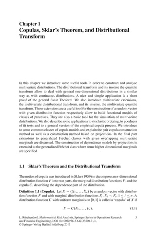
  • 4. 6 1 Copulas, Sklar’s Theorem, and Distributional Transform Figure 1.1 Copula of 1 uniform distribution on line segments (published in: Journal of Stat. Planning Inf., 139: 3921–3927, 2009) 1 2 1 1 2 randomizations V at the jumps or in the components, i.e. choosing Ui D Fi .Xi ; Vi /, may introduce artificial local dependence between the components of a random vector on the level of the copula. From the copula alone one does not see whether some local positive or negative dependence is a real one or just comes from the choice of the copula. For dimension n D 2 the copula in Figure 1.1 could mean a real switch of local positive and negative dependence for the original distribution, but it might also be an artefact resulting from the randomization in case the marginals are e.g. both two-point distributions while the joint distribution in this case could be even comonotone. Thus the copula information alone is not sufficient to decide all dependence properties. (b) Conditional value at risk. A more recent application of the distributional trans- form is to risk measures. It is well known that the conditional tail expectation TCE˛ .X / WD E.X j X Ä q˛ /; (1.10) where q˛ is the lower ˛-quantile of the risk X , does not define a coherent risk measure except when restricted to continuous distributions. This defect can be overcome by using the distributional transform U D F .X; V / and defining the modified version, which we call conditional value at risk (CVR˛ ) CVR˛ .X / D E.X j U Ä ˛/: (1.11) By some simple calculations (see Burgert and R¨ (2006b)) one sees that u 1 CVR˛ .X / D EX1.X < q˛ / C q˛ ˛ P .X < q˛ / D ES˛ .X /: ˛ (1.12) Thus the more natural definition of CVR˛ coincides with the well-established “expected shortfall risk measure” ES˛ .X / which is a coherent risk measure.
  • 5. 1.2 Copula Models and Copula Constructions 7 As a consequence the expected shortfall is represented as conditional expec- tation and our definition in (1.11) of the conditional value at risk seems to be appropriate for this purpose. (c) Stochastic ordering. The construction of copulas based on the distributional transform as in the proof of Sklar’s Theorem above has been used in early papers on stochastic ordering. The following typical example of this type of result is from R¨ (1981b, Proposition 7). u Proposition 1.6. Let Fi , Gi be one-dimensional distribution functions with Fi Ä Gi (or equivalently Gi Äst Fi ), 1 Ä i Ä n. Then to any F 2F .F1 ; : : : ; Fn / there exists an element G 2 F .G1 ; : : : ; Gn / with G Äst F . Here Äst denotes the multivariate stochastic ordering w.r.t. increasing functions. Proof. Let X D .X1 ; : : : ; Xn / F and let Ui D Fi .Xi ; V / denote the distri- butional transforms of the components Xi . Then U D .U1 ; : : : ; Un / is a copula vector of F . Define Y D .Y1 ; : : : ; Yn / as vector of the quantile transforms of the components of U , Yi D Gi 1 .Ui /. Then Y G 2 F .G1 ; : : : ; Gn / and from the assumption Fi Ä Gi we obtain that Y Ä X pointwise. In consequence G Äst F . In particular the above argument shows that G Äst F if F and G have the same copula. ˙ 1.2 Copula Models and Copula Constructions In order to construct a distributional model for a random vector X it is by Sklar’s representation theorem sufficient to specify a copula model fitting to the normalized data. There are a large number of suggestions and principles for the construction of copula models. Classical books on these models for n D 2 are Mardia (1962) and Hutchinson and Lai (1990). More recent books for n 2 are Joe (1997), Nelsen (2006), Mari and Kotz (2001), Denuit et al. (2005), and McNeil et al. (2005b). A lot of material on copulas can also be found in the conference volumes of the “Probability with given marginals” conferences – i.e. the series of conferences in Rome (1990), Seattle (1993), Prague (1996), Barcelona (2000), Qu´ bec (2004), e Tartu (2007) and Sao Paulo (2010) as well as in the recent proceedings edited by Jaworski, Durante, H¨ rdle, and Rychlik (2010). A huge basket of models has a been developed and some of its properties have been investigated, concerning in particular the following questions: • What is the “range of dependence” covered by these models and measured with some dependence index. Is the range of dependence wide and flexible enough? • What models exhibit tail dependence and thus are able to model situations with strong positive dependence in tails? • Is some parameter available describing the degree of dependence?
  • 6. 8 1 Copulas, Sklar’s Theorem, and Distributional Transform • Is there a natural probabilistic representation respectively interpretation of these models describing situations when to apply them? • Is there a closed form of the copula or a simple simulation algorithm so that goodness of fit test can be applied to evaluate whether they fit the data? Several questions of this type have been discussed in the nice survey papers of Schweizer (1991) and Durante and Sempi (2010). 1.2.1 Some Classes of Copulas Copulas, their properties and applications are discussed in detail in the above- mentioned literature. Copulas are not for any class of distributions the suitable standardizations as for example for elliptical distributions. In extreme value theory a standardization by the exponential distribution may be better adapted. For some applications it may be more natural and simpler to model the distributions or their densities directly without referring to copulas. Conceptually and for some investigation of dependence properties like tail-dependence the notion of copula is however a useful tool. Some classical classes of copulas are the following. • The “Farlie–Gumbel–Morgenstern (FGM) copula”: C˛ .u; v/ D uv.1 C ˛.1 u/.1 v//; j˛j Ä 1 (1.13) as well as its generalized versions, “EFGM copulas” are extensions of FGM to the n-dimensional case and given by ! Q n X Q C.u/ D ui 1 C ˛T j 2T .1 uj / (1.14) i D1 T f1;:::;ng for suitable ˛T 2 R1 . • The “Archimedean copulas” Cˆ .u1 ; : : : ; un / D ˆ 1 .ˆ.u1 / C C ˆ.un // (1.15) for some generator ˆ W .0; 1 ! RC with ˆ.1/ D 0 such that ˆ is com- pletely monotone. In fact Cˆ is an n-dimensional copula if and only if ˆ is “n-monotone”, i.e. ˆ is .n 2/ times differentiable and . 1/k ˆ.k/ .t/ 0; 0ÄkÄn 2; 8t > 0 (1.16) and . 1/n 2 ˆ.n 2/ is decreasing and convex (see McNeil and Neˇlehov´ (2010)). s a
  • 7. 1.2 Copula Models and Copula Constructions 9 In case ˆ.t/ D ˛ .t 1 ˛ 1/ one gets the “Clayton copula” X Á 1=˛ C˛ .u/ D ui ˛ nC1 ; ˛ > 0: (1.17) In case ˆı .t/ D 1 ı log.1 .1 e ı /e t / one gets the “Frank copula”  Qn ıui à 1 i D1 .e 1/ Cı .u/ D log 1 C : (1.18) ı .e ı 1/n 1 ˆ is by Bernstein’s theorem completely monotone if and only if it is n-monotone for all n 2 N. Archimedean copulas are connected with mixing models (“frailty models”). Let Z Y n FX .x/ D .Gi .xi //ı dF‰ .ı/; i D1 where ‰ is a positive real mixing variable. Then with L‰ , the Laplace transform of ‰, we obtain that the i -th marginal is given by Z Fi .xi / D exp.ı ln Gi .xi //dF‰ .ı/ D L‰ . ln Gi .xi //: As a consequence one gets ÂX n à FX .x/ D L‰ 1 L‰ .Fi .xi // ; (1.19) i D1 i.e. a representation as in (1.15) holds with the generator ˆ D L‰ which by Bernstein’s theorem is completely monotone. Archimedean copulas arise from multivariate distributions that have a stochas- tic representation of the form d X DR U (1.20) U whereP is uniformly distributed on the unit simplex (1-sphere) in fx 2Rn , C n Rn I C i D1 xi D 1g respectively the simplex in Rn , and R is a scaling random variable with values in RC independent of U . Formulae for the relation between the distribution function FR and the generator ˆ are available (see McNeil and Neˇlehov´ (2010)). s a • “Elliptical distributions” arise from stochastic representations of the form XD C RAU; (1.21) where U is uniformly distributed on the unit 2-sphere Sn 1 D fx 2 Rn ; Pn i D1 ui D 1g in R . R is a real positive random variable independent from 2 n U and A is an n n-matrix. X has a density of the form
  • 8. 10 1 Copulas, Sklar’s Theorem, and Distributional Transform f .x/ D j†j 1 ˆ..x /> † 1 .x // with † D AA> : The distribution is denoted as E. ; †; FR /. Multivariate normal distributions are elliptical (or elliptically contoured). The copulas of elliptical distributions are in general not available in closed form. • “Extreme value copulas” are defined as possible limits of max sequences. Let Xi D .Xi;1 ; : : : ; Xi;d /, 1 Ä i Ä n (note that here d D dimension but n D sample index) be a sequence of iid random vectors with copula CF . Let Mn D maxfX1 ; : : : ; Xn g D .Mn;1 ; : : : ; Mn;d / be the componentwise max of the Xi , then the copula Cn of Mn is given by n 1=n 1=n Cn .u/ D CF .u1 ; : : : ; ud /: C is called an “extreme value copula” if for any n 2 N there exist some copula CF such that n 1=n 1=n C D CF .u1 ; : : : ; ud /: (1.22) A well-known fact is: C is an extreme value copula if and only if C is “max stable”, i.e. C.u/ D m 1=m 1=m C .u1 ; : : : ; ud / for all m 2 N. De Haan and Resnick (1977) and Pickands (1981) gave the following representation of extreme value copulas: C is an extreme value copula if and only if it has a representation of the form C.u/ D exp. l. log u1 ; : : : ; log ud //: (1.23) Here the “tail dependence function” l W .0; 1/d ! Œ0; 1 is given by Z l.x/ D max.wj xj /dH.w/ (1.24) Sd 1 j Äd R where H is a measure on the simple Sd 1 satisfying Sd 1 wj dH.w/ D 1, 1 Ä j Ä d . H is called the “spectral measure” of C . An example of copulas which are of interest in extreme value theory are “Gumbel copulas” given by  X n Á1=ı à Cı .u/ D exp . log ui /ı (1.25) i D1 for ı 2 Œ1; 1/. Gumbel copulas are extreme value copulas. The parameter ı is a dependence parameter. If 1 Ä ı1 < ı2 , then Gı2 is more strongly dependent (in the sense of supermodular ordering) than Gı1 (see Wei and Hu (2002)).
  • 9. 1.2 Copula Models and Copula Constructions 11 1.2.2 Copulas and L2 -Projections A general principle for the construction of dependence models (copulas) was introduced in R¨ (1985). It is based on the following representation result. Let u Cn .λ n / denote the set of all copulas on Œ0; 1n which are Lebesgue-continuous and n thus have Lebesgue-densities f . Let Cn .λ n / be the set of all signed measures on s n n Œ0; 1 with uniform marginals and which have Lebesgue-densities f . For any integrable f 2 L1 .Œ0; 1n ; λ n / and T n f1; : : : ; ng we define Z Q fT D f i 2T dyi ; (1.26) i.e. we integrate over the components in T . We consider fT as a real function on Œ0; 1n being constant in the T components. The following linear operator S W L1 .λ n / ! L1 .λ n / is of interest, n n X Sf D f fT C .n 1/ff1;:::;ng (1.27) T f1;:::;ng jT jDn 1 since it leads to the following representation result. Theorem 1.7 (Copulas and L2 -projections). All probability distributions on Œ0; 1n with Lebesgue-density and uniform marginals are of the form .1 C Sf /λ n n where f 2 L1 .λ n /, more precisely n ˚ « Cn .λ n / D Q D .1 C Sf /λ n I f 2 L1 .λ n / s n n n (1.28) and ˚ « Cn .λ n / D P D .1 C Sf /λ n I f 2 L1 .λ /; Sf n n n 1 : (1.29) Proof. Any P 2 Cn .λ n / has by the Radon–Nikod´ m theorem a density of the s n y form P D .1 C f /λ n where fT D 0 for jT j n 1. This implies that Sf D f , n i.e. P D .1 C Sf /λ n . Conversely, let f 2 L1 .λ n / and P D .1 C Sf /λ n . Then for n n n T0 f1; : : : ; ng, jT0 j D n 1 and any further T f1; : : : ; ng with jT j D n 1, T 6D T0 we have .fT /T0 D ff1;:::;ng and, therefore,  X à .Sf /T0 D f fT0 fT C .n 1/ff1;:::;ng (1.30) jT jDn 1 T0 T 6DT0 X D fT0 fT0 .fT /T0 C .n 1/ff1;:::;ng D 0: (1.31) jT jDn 1 T 6DT0
  • 10. 12 1 Copulas, Sklar’s Theorem, and Distributional Transform Therefore Q D .1 C Sf /λ n 2 Cn .λ n /. This implies (1.28). Equation (1.29) is n s n immediate from (1.28). The operator S in (1.27) can be considered as an L2 -projection of a (signed) measure Q D .1 C f /λ n , f 2 L1 .λ 1 / to a copula P D .1 C Sf /λ n if Sf n n n 1. The basic idea of the construction method for dependence (copula) models in R¨ u (1985) is to describe in a first step the relevant dependence by the density function 1 C f . In a second step this model Q D .1 C f /λ n is projected to the class of n copulas in the form P D .1 C Sf /λ n .n The resulting proposed model construction method is the following: Construction by “projection method”: Let f# , # 2 ‚ be a parametric family of functions in L1 .λ n / (describing the intended dependence structure) such that n Sf# 1, # 2 ‚. Then the proposed model obtained by the projection method is given by ˚ « P D P# D .1 C Sf# /λ n I # 2 ‚ : n (1.32) The inherent idea in this construction is the hope that the projection on the correct marginal structure does not change the intended dependence structure too much. Obviously we can use the same procedure as above also for the construction of elements in the Fr´ chet class M.P1 ; : : : ; Pn / which are continuous w.r.t. a product e measure 1 ˝ ˝ n . This projection idea is also underlying Sklar’s representation theorem. Let G 2 Fn .G1 ; : : : ; Gn / be a multivariate distribution function with marginals G1 ; : : : ; Gn and with copula C . Assume that G is a good description of the dependence structure for a model. At the same time assume that the correct marginals should be F1 ; : : : ; Fn instead of G1 ; : : : ; Gn . Then by Sklar’s Theorem the following “nonmetric projection” would seem natural: G ! C ! F D C.F1 ; : : : ; Fn /: (1.33) By this transition the dependence structure is retained in the copula C . The difficulty of calculation may however prevent use of this transition in examples. Typically it will be easier to calculate (only) densities. The following examples illustrate the projection method, see R¨ (1985) and Mari u and Kotz (2001, pp. 73–78). ˚ « Example 1.8. Let f 2 L1 .λ n /, let ˛0 D inf .Sf /.x/I x 2 Œ0; 1n > 1 and n consider f# .x/ D #f .x/, # 2 Œ0; j˛0 j . 1 Q R (1) Generalized FGM-family: If f .x/ D nD1 vi .xi / where vi .xi /dxi D 0, i 1 Ä i Ä n, then Sf D f and P gives a “generalized FGM-family” (see Johnson and Kotz (1975) and KimeldorfQ Sampson (1975a,b), and (1.13)). and (2) Polynomial copula models: If f .x/ D nD1 ximi is a polynomial, then i ! Q n X n Q 1 Q n 1 Sf .x/ D ximi ximi C .n 1/ (1.34) i D1 i D1 j 6Di mj C 1 i D1 mi C 1
  • 11. 1.2 Copula Models and Copula Constructions 13 gives a “polynomial copula model” which is the same as the FGM-model generated by vi .xi / D ximi mi1 . Linear combinations then yield the general C1 form of polynomial copula models. The restrictions to the parameters are given in Mari and Kotz (2001, p. 74). This polynomial model has also been discussed in Wei, Fang, and Fang (1998). Several families of polynomial copulas have been suggested as local approximations of other copula families. So the Ali–Mikhail–Haq family is a polynomial approximate in the neighbourhood of the independence copula, the FGM is an approximation of the Plackett family (see Mari and Kotz (2001, p. 75)). (3) A copula concentrated strongly near the diagonal: Let n D 2 and consider f .x; y/ D p 1 . The function f has singularities at the diagonal, i.e. we jx yj expect a large density in the neighbourhood of the diagonal. Then by simple calculation one gets 1 p p p p Á 8 Sf .x; y/ D p 2 xC 1 xC yC 1 y C : (1.35) jx yj 3 P describes a family of copulas which is concentrated near the diagonal. # is a positive dependence parameter; higher values of # yield higher order positive dependence. (4) Diagonal weakly concentrated copula: For ‚ D Œ0; 1, n D 2 define f# .x; y/ D 1fjx yj>#g ; so .1 C f# /λ 2 is concentrated in a neighbourhood of the diagonal but it is n uniformly distributed on f.x; y/ 2 Œ0; 12 W jx yj Ä #g in contrast to the singular concentration in Example 1.8, (1.8). By the projection to the correct marginals we obtain Sf# .x; y/ D f# .x; y/ C g# .x/ C g# .y/ .1 #/2 ; (1.36) where g# .x/ D .2 2#/1f#ÄxÄ1 #g C .1 x y/1.0Äx<#/ .x y/1.x>1 #/ 1 for 0 Ä # Ä 2 and g# .x/ D .x #/1.x>#/ C .# x/1.x<1 #/ , 1 < # Ä 1. 2 The projected probability model P# D .1 C Sf# /λ 2 approaches for # ! 1 n the product measure while for # small (neglecting small and large x-values) ( 2 2# for jx yj < #; 1 C .Sf# /.x; y/ (1.37) 1 2# for jx yj > #:
  • 12. 14 1 Copulas, Sklar’s Theorem, and Distributional Transform In order to introduce a stronger dependence effect one can start with f#;a .x; y/ D af# .x; y/ which for # small and a large centres the distribution near the diagonal. ˙ 1.3 Multivariate Distributional and Quantile Transform The distributional transform F .X; V / as well as the inverse quantile transform F 1 .V / have been generalized to the multivariate case. Definition 1.9 (Multivariate quantile transform). Let F be a d -dimensional distribution function and let V1 ; : : : ; Vn be iid U.0; 1/-distributed random variables. Then the “multivariate quantile transform” Y WD F 1 .V / is defined recursively as Y1 WD F1 1 .V1 / (1.38) Yk WD Fkj1;:::;k 1 .Vk j Y1 ; : : : ; Yk 1 /; 1 2 Ä k Ä n; where Fkj1;:::;k 1 denote the conditional distribution functions of the k-th component k given the first k 1 components 1 ; : : : ; k 1 . The multivariate quantile transform is a basic method to construct a random vec- tor Y with specified distribution function F from a given vector V D .V1 ; : : : ; Vn / of iid uniformly on Œ0; 1 distributed random variables. By construction the mul- tivariate quantile transform uses only one-dimensional conditional distribution functions. Theorem 1.10 (Multivariate quantile transform). The multivariate quantile transform Y D F 1 .V / is a random vector with distribution function F . Proof. In case n D 2 and for any x1 ; x2 2 R we have using the independence of .Vi / Z x1 P .Y1 Ä x1 ; Y2 Ä x2 / D P .Y2 Ä x2 j Y1 D y1 /dF1 .y1 / 1 Z x1 D P .F2j11 .V2 j y1 / Ä x2 j Y1 D y1 /dF1 .y1 / 1 Z x1 D P .F2j11 .V2 j y1 / Ä x2 /dF1 .y1 / 1 Z x1 D F2j1 .x2 j y1 /dF1 .y1 / D F12 .x1 ; x2 /: 1 By induction this argument extends to yield P .Y1 Ä x1 ; : : : ; Yn Ä xn / D F .x1 ; : : : ; xn /.
  • 13. 1.3 Multivariate Distributional and Quantile Transform 15 The multivariate quantile transform was introduced in O’Brien (1975), Arjas and Lehtonen (1978), and R¨ (1981b). The construction Y is an inductive construction u of a random vector with specified distribution function F and is called “regression representation” since Y is of the form Y1 D h1 .V1 /; Y2 D h2 .Y1 ; V2 /; Y3 D h2 .Y1 ; Y2 ; V3 /; (1.39) : : : Yn D hn .Y1 ; : : : ; Yn 1 ; Vn / representing Yk as function of the past Y1 ; : : : ; Yk 1 and some innovation Vk . As a consequence this implies the “standard representation” Yk D fk .V1 ; : : : ; Vk /; 1 Ä k Ä n: (1.40) The multivariate quantile transform and particularly Theorem 1.10 is a basic method for the “simulation of multivariate distributions”. In order to construct a random vector with distribution function F one needs to simulate iid U.0; 1/- random variables and to determine the inverses of the one-dimensional conditional distribution functions Fi jx1 ;:::;xi 1 .xi /, which can be done in many examples either analytically or numerically. There is a large literature on (Monte Carlo) simulation of multivariate distributions, which uses essentially the multivariate quantile trans- form. This transform was introduced first in the above-mentioned papers dealing with representation of stochastic sequences and with stochastic orderings. Definition 1.11 (Multivariate distributional transform). Let X be an n- dimensional random vector and let V1 ; : : : ; Vn be iid U.0; 1/-distributed random variables, V D .V1 ; : : : ; Vn /. For λ D .λ1 ; : : : ; λn / 2 Œ0; 1n define F .x; λ/ WD F1 .x1 ; λ1 /; F2 .x2 ; λ2 j x1 /; : : : ; Fd .xd ; λd j x1 ; : : : ; xd 1/ ; (1.41) where F1 .x1 ; λ1 / D P .X1 < x1 / C λ1 P .X1 D x1 /; Fk .xk ; λk j x1 ; : : : ; xk 1/ D P .Xk < xk j Xj D xj ; j Ä k 1/ C λk P .Xk D xk j Xj D xj ; j Ä k 1/ are the distributional transforms of the one-dimensional conditional distributions. Finally the “multivariate distributional transform”of X is defined as U WD F .X; V /: (1.42)
  • 14. 16 1 Copulas, Sklar’s Theorem, and Distributional Transform Rosenblatt (1952) introduced this transformation in the special case of absolutely continuous conditional distributions allowing the application of the transformation formula. Therefore this transformation is also called the “Rosenblatt transforma- tion” in this case. For general distributions the multivariate distributional transform (generalized Rosenblatt transform) was introduced in R¨ (1981b). The basic u property is stated in the following theorem in R¨ (1981b). u Theorem 1.12 (Multivariate distributional transform). Let X be a random vec- tor and let U D F .X; V / denote its multivariate distributional transform. Then (a) U U..0; 1/d /; (1.43) i.e. the components Ui of U are iid U.0; 1/ distributed. 1 (b) The multivariate quantile transform F is inverse to the multivariate distribu- tional transform, i.e. XD F 1 .U / D F 1 . F .X; V // a.s. (1.44) Proof. U1 D F1 .X1 ; V1 / U.0; 1/ by Proposition 1.3. Consider next U2 D F2 .X2 ; V2 j X1 /. Conditionally given X1 D x1 we have again from Proposition 1.3 that d U2 D F2 .X2 ; V2 j x1 / U.0; 1/: Furthermore, P U2 jX1 Dx1 D U.0; 1/ is independent of x1 and thus U2 , X1 are independent. Since U1 D F1 .X1 ; V1 / we get from iterated conditional expectation that also U2 , U1 are independent. The general case then follows by induction. Remark 1.13 (Regression and standard representation). (a) By combining the multivariate quantile and the multivariate distributional trans- form one gets for any given stochastic sequence .Xk / a pointwise “standard (innovation) representation” Xk D fk .U1 ; : : : ; Uk / a.s.; (1.45) respectively a pointwise “regression representation” Xk D fk .X1 ; : : : ; Xk 1 ; Uk / a.s.; 1ÄkÄn (1.46) with some iid sequences .Ui /, Ui U.0; 1/. This result was proved first for n D 2 in Skorohod (1976). Related functional representations of classes of stochastic models are given in R¨ and de Valk (1993). For example in the case of u Markov chains the regression representation reduces to the following functional representation of (any) Markov chain: Corollary 1.14 (Regression representation of Markov chains). Any Markov chain .Xn / has a representation as a nonlinear regression model
  • 15. 1.4 Pair Copula Construction of Copula Models 17 Xk D fk .Xk 1 ; Uk / a.s.; (1.47) where .Uk / is an iid sequence of U.0; 1/-distributed random variables, Uk is independent of X1 ; : : : ; Xk 1 . (b) The copula transformation X D .X1 ; : : : ; Xd / ! U D .U1 ; : : : ; Ud /; Ui D Fi .Xi ; Vi / which transforms a vector X to a copula vector U , where U corresponds to the copula of X , forgets about the marginals but retains essential information on the dependence structure of X . On the contrary the multivariate distribu- tional transform forgets also about the dependence structure. This is an interest- ing property, when one wants to identify a distribution. These two different properties of the copula transformation and the multivariate distributional transform lead to different kinds of applications. Some of them are described in Section 1.5. ˙ 1.4 Pair Copula Construction of Copula Models Besides the multivariate quantile transform in Theorem 1.10, which is based on the one-dimensional conditional distributions Fi jx1 ;:::;xi 1 , several further methods to represent a distribution function F in terms of conditional distribution functions have been proposed. Particular interest in the recent literature and in various applications arose from the “pair copula construction (PCC)” method which is based on a series of certain (organized) pairs of variables. In the original example Joe (1997) used the following pairwise construction of an m-dimensional distribution function F . For m D 3, F D F123 can be represented as Z x2 F123 .x/ D F13jz2 .x1 ; x3 /dF2 .z2 / (1.48) 1 where F13jz2 is the conditional distribution function of the pair X1 ; X3 given X2 D z2 . By Sklar’s Theorem this can also be written in terms of the conditional copula C13jz2 in the form Z x2 F123 .x/ D C13jz2 .F1jz2 .x1 /; F3jz2 .x3 //dF2 .z2 /: (1.49) 1 Similarly for general m one obtains recursively the representation Z x2 Z xm 1 F1:::m .x/ D ::: C1mjz2 ;:::;zm 1 F1jz2 ;:::;zm 1 .x1 /; 1 1 (1.50) Fmjz2 ;:::;zm 1 .xm / dF2:::m 1 .z2 ; : : : ; zm 1 / which is given in terms of pairwise conditional copulas.
  • 16. 18 1 Copulas, Sklar’s Theorem, and Distributional Transform In Bedford and Cooke (2001, 2002) and Kurowicka and Cooke (2006) some general classes of graphical organization principles representing multivariate distri- butions were developed. See also the survey of Czado (2010). Two basic examples of these classes of constructions are C -vines and D-vines (C D canonical, D D drawable). (a) D-vines: The construction of D-vines is based on densities and uses the representation Y n f .x1 ; : : : ; xn / D fi jx1 ;:::;xi 1 .xi /f1 .x1 /: (1.51) i D2 By Sklar’s Theorem we have f12 .x1 ; x2 / D c12 .F1 .x1 /; F2 .x2 //f1 .x1 /f2 .x2 /; (1.52) where c12 is a bivariate copula density. This implies for the conditional density f1jx2 .x1 / D c12 .F1 .x1 /; F2 .x2 //f1 .x1 /: (1.53) Using (1.53) for the conditional density of .X1 ; Xi / given X2 ; : : : ; Xi 1 we obtain by recursion fi jx1 ;:::;xi 1 .xi / D c1;i j2;:::;i 1 fi jx2 ;:::;xi 1 .xi / ! Y i 2 D cj;i jj C1;:::;i 1 ci 1;i fi .xi / (1.54) j D1 using the conditional copula densities cj;i jj C1;:::;i 1 D cj;i jxj C1 ;:::;xi 1 .Fj jxj C1 ;:::;xi 1 .xj /; Fi jxj C1 ;:::;xi 1 .xi //: As a result we obtain the “D-vine” density decomposition ! YY n i 2 Y n Y n f .x1 ; : : : ; xn / D cj i jj C1;:::;i 1 ci 1;i fl .xl / i D2 j D1 i D2 lD1 n 1Y ! Yn i Y n D cj;i Cj j.j C1;:::;j Ci 1/ fl .xl /: (1.55) i D1 j D1 lD1 The conditional copula densities in (1.55) are evaluated at the conditional distribution functions Fj jxj C1 ;:::;xj Ci 1 ; Fi Cj jxj C1 ;:::;xj Ci 1 .
  • 17. 1.4 Pair Copula Construction of Copula Models 19 § ¤ § ¤ § ¤ § ¤ § ¤ 1 2 3 4 5 T1 ¦ ¥ ¨¦ ¥ ¨¦ ¥ ¨¦ ¥ ¨¦ ¥ 12 23 34 45 T2 © ¨ © ¨ © ¨ © 13 j 2 24 j 3 35 j 4 T3 © ¨ © ¨ © 14 j 23 25 j 34 T4 © © ¨ 15 j 234 T5 © Figure 1.2 D-vine tree for n D 5 The D-vine decomposition in (1.55) can be organized iteratively by pairwise copulas using iteratively levels T1 ; : : : ; Tn 1 . For n D 5 we obtain the represen- tation f .x1 ; : : : ; x5 / Y 5 D fl .xl /c12 c23 c34 c45 c13j2 c24j3 c35j4 c14j23 c25j34 c15j234 : lD1 This is described in the following graphical organization. Each transition step from level Ti to level Ti C1 involves a (conditional) pair copula (Figure 1.2). (b) C -vines: C -vine decompositions are obtained when applying the representa- tion of the conditional density successively to the conditional distribution of Xi 1 ; Xi given X1 ; : : : ; Xi 2 . This gives fi jx1 ;:::;xi 1 .xi / D ci 1;i jx1 ;:::;xi 2 fi jx1 ;:::;xi 1 .xi /: (1.56) Using (1.56) instead of (1.54) in (1.51) we obtain the C -vine decomposition YY n i 1 f .x1 ; : : : ; xn / D f1 .x1 / ci k;i j1;:::;i k 1 fk .xi / i D2 kD1 ! Yk 1 n Y Y n D ci k;i j1;:::;i k 1 fk .xk / i D2 kD1 kD1 ! YY n 1n j Y n D cj;j Ci j1;:::;j 1 fk .xk /: (1.57) j D1 i D1 kD1
  • 18. 20 1 Copulas, Sklar’s Theorem, and Distributional Transform § ¤ ¨ ¦ ¥ 2 12 j 1 © § ¤ 13 § ¤ ((( 3 (( 3 ¨ 23 ¨ ( 1 ( ¦ ¥ 25 j 1 T1 : 1 ` T2 : ¦ ¥ ``5 `` 1 12 15 Z 1 ` © 24 j b © Z4 ``` § ¤ b 1 ¨ ` 5 b Z ¦ ¥ b 14 Z § ¤ © Z 4 ¦ ¥ ¨ j12 25 j 1 ¨ 35 © ¨ ¨ 45 j 123 23 j 1 a 34 j 34 j 12 35 j 12 ©aaa T3 : T4 : 12 © © aa ¨ 24 j 1 © Figure 1.3 C -vine for n D 5 For n D 5 (1.57) gives a decomposition of the form Y 5 f .x1 ; : : : ; x5 / D fk .xk /c12 c13 c14 c15 c23j1 c24j1 c25j1 c34j12 c35j12 c45j123 ; kD1 which is represented by the following graph in Figure 1.3 with levels T1 ; : : : ; T4 . Again each transition of level Ti to Ti C1 involves (conditional) pair copulas. Remark 1.15. (a) PCC and Markov random fields: More general systems to organize pairwise conditional copulas in order to represent uniquely an n-dimensional distribution function respectively density are described in Bedford and Cooke (2001, 2002) and Kurowicka and Cooke (2006) under the denomination “regular vine”. These decompositions are represented graphically as a nested tree. Edges of the tree denote the indices used in the conditional copula densities. The representation of the density in terms of these conditional distributions is an analogue of the Hammersley– Clifford theorem for Markov random field specifications by certain conditional distributions (of the components given their neighbourhoods). Depending on the choice of the neighbourhoods there is some strong similarity between both ways of constructing multivariate (spatial) models. (b) Reduction of vine representation: Haff, Aas, and Frigessi (2010) consider a reduction of the (great) complexity of regular vine models by assuming that the conditional copula densities cj;i Cj jj C1;:::;j Ci 1 respectively copulas C1j j2;:::;j 1 do not depend on the var- iables xk in the condition but they depend only through the conditional distribution functions Fj jxj C1 ;:::;xj Ci 1 etc. This reduction seems to yield good approximations in several applications. ˙
  • 19. 1.5 Applications of the Distributional Transform 21 1.5 Applications of the Distributional Transform 1.5.1 Application to Stochastic Ordering Let Äst denote the usual stochastic ordering on Rn , i.e. the integral induced ordering w.r.t. the class Fi of increasing functions which is defined by X Äst Y if Ef .X / Ä Ef .Y / for all f 2 Fi (1.58) such that the expectations exist. The following sufficient condition for the multitivariate stochastic order is a direct consequence of Theorem 1.10 on the multivariate quantile transform. Proposition 1.16. Let X , Y be n-dimensional vectors with distribution functions F , G 2 Fn and let .Vi /1Äi Än be iid, U.0; 1/-distributed, then F 1 .V / Ä G 1 .V / implies that X Äst Y: (1.59) Condition (1.59) is stated in R¨ (1981b). It implies various sufficient conditions u for stochastic ordering going back to classical results of Veinott (1965), Kalmykov (1962), and Stoyan (1972). The comparison result of Veinott (1965) states Corollary 1.17 (Comparison w.r.t. stochastic order Äst ). Let X , Y be n-dimen- sional random vectors such that X1 Äst Y1 and for 2 Ä i Ä n P Xi jX1 Dx1 ;:::;Xi 1 Dxi 1 Äst P Yi jY1 Dy1 ;:::;Yi 1 Dyi 1 (1.60) for all xj Ä yj , 1 Ä j Ä i 1, then X Äst Y: Proof. Condition (1.60) implies (by induction) that F 1 .V / Ä G 1 .V / where F D d d FX , G D FY . Since F 1 .V / D X and G 1 .V / D Y this implies X Äst Y . The standard construction in (1.45) respectively the regression representation in (1.46) however are not applicable in general when P Äst Q, i.e. they do not in general produce pointwise a.s. constructions X P, Y Q such that X Ä Y a.s. The existence of such a coupling is however true under general conditions as follows from the following theorem due to Strassen (1965). Let .S; Ä/ be a Polish space supplied with a closed semiorder “Ä”, i.e., the set f.x; y/ 2 S S I x Ä yg is closed w.r.t. the product topology. The closed order Ä induces the “stochastic order” Äst on the set M 1 .S / of probability measures on S defined by
  • 20. 22 1 Copulas, Sklar’s Theorem, and Distributional Transform Z Z P Äst Q if f dP Ä f dQ (1.61) for all integrable increasing real functions f 2 Fi D Fi .S; Ä/: Theorem 1.18 (Strassen’s ordering theorem, Strassen (1965)). Let .S; Ä/ be a Polish space supplied with a closed partial order. Let P; Q 2 M 1 .S /, then P Äst Q , There exist random variables X P; Y Q such that X Ä Y a.s. In Section 3.4 we will discuss extensions of this a.s. ordering theorem to the class of “integral induced orderings ÄF ” for some function class F . These are defined via Z Z P ÄF Q if f dP Ä f dQ for all integrable f 2 F : Early sources for integral induced orderings are Marshall and Olkin (1979), R¨ u (1979), and Whitt (1986). The regression and standard constructions are used essentially in various papers and textbooks on stochastic ordering and are closely connected with some notions of stochastic ordering respectively dependence orderings. We state as one example the notion of conditional increasing in sequence (CIS). Definition 1.19 (Conditional increasing in sequence (CIS)). A random vector X D .X1 ; : : : ; Xn / is called “conditional increasing in sequence” (CIS)if for 2 Ä i Ä n Xi st .X1 ; : : : ; Xi 1 /; (1.62) i.e. the conditional distribution Pi jx1 ;:::;xi 1 D P Xi jX1 Dx1 ;:::;Xi 1 Dxi 1 is stochastically increasing in .x1 ; : : : ; xi 1 /. The CIS-property of a random vector X is a positive dependence property of X . This property is equivalent to the condition that the standard representation based on the multivariate quantile transform Y D F 1 .V / is an increasing function in V , i.e. Yk D fk .V1 ; : : : ; Vk / are increasing in V; 2 Ä k Ä n: (1.63) Proposition 1.20 (CIS and multivariate quantile transform). Let X be a random vector with distribution function F , then X is CIS if and only if the construction by the multivariate quantile transformation Y D F 1 .V / D .f1 .V1 /; f2 .V1 ; V2 /; : : : ; fn .V1 ; : : : ; Vn // is monotonically increasing in V .
  • 21. 1.5 Applications of the Distributional Transform 23 1.5.2 Optimal Couplings The multivariate quantile transform is by Theorems 1.10 and 1.12 a basic con- struction method for random vectors. An extension of this construction leads to interesting connections with the construction of (optimal) couplings of distributions. Let h W Rn ! Rm be a measurable function and let P 2 M 1 .Rn ; Bn / have distribution function F . Let furthermore S , V be random variables on . ; A; R/ such that the “distributional equation” P h D RS ; holds, i.e. h and S have the same distributions w.r.t. P respectively R. Theorem 1.21 (Solution of stochastic equations, Ru (1985) and Rachev and Ru ¨ ¨ (1991)). Let S be a random variable on a probability space . ; A; R/ that satisfies the distributional equation P h D RS : Assume that V D .Vi /1Äi Än are further iid U.0; 1/-distributed random variables on . ; A; R/ such that S , V are independent. Then there exists a random variable X on . ; A; R/ such that (a) RX D P , i.e. X has distribution function F and (b) X is a solution of the “stochastic equation” h ı X D S a.s. with respect to R: Remark 1.22. The situation is described by the following diagram: S . ; A; R/ .Rm ; Bm / X h .Rn ; Bn ; P / If the distributional equation RS D P h holds, then there exists a solution X with RX D P solving the stochastic equation h ı X D S a.s. and thus making the diagram commutative. ˙ Proof. We denote by i j 1 Dx1 ;:::; i 1 Dxi Fi jx1 ;:::;xi 1 ;s D Fi . j x1 ; : : : ; xi 1 ; s/ DP 1 ;hDs the conditional distribution function of the i -th projection i given j D xj , j Ä i 1 and given h D s and define inductively a random vector X by
  • 22. 24 1 Copulas, Sklar’s Theorem, and Distributional Transform X1 D F1 1 .V1 j S /; X2 D F2 1 .V2 j X1 ; S /; : : : ; (1.64) Xn D Fn 1 .Vn j X1 ; : : : ; Xn 1 ; S /: Equation (1.64) is an extension of the multivariate quantile transform. By the independence assumptions we obtain RX1 jS Ds D RF1 1 .V jS /jS Ds 1 .V jS Ds/ 1 jhDs 1 D R F1 1 DP : Similarly, 1 RX2 jX1 Dx1 ;S Ds D RF2 .V2 jX1 ;S /jX1 Dx1 ;S Ds 1 .V2 jx1 ;s/ 2 j 1 Dx1 ;hDs D R F2 DP implying Z R.X1 ;X2 /jS Ds D RX2 jX1 Dx1 ;S Ds dRX1 jS Ds Z 2 j 1 Dx1 ;hDs 1 jhDs D P dP .x2 / D P . 1 ; 2 /jhDs : By induction we find RX jS Ds D P jhDs and, therefore, RX D P . Since almost surely w.r.t. P h it holds that P jhDs .fxI h.x/ D sg/ D 1 we obtain X jS Ds R .fxI h.x/ D sg/ D 1ŒRS  and thus Z R.fh.X / D S g/ D RX jS Ds .fxI h.x/ D sg/dRS .x/ D 1: Remark 1.23. Using a measure isomorphism argument Theorem 1.21 on the solutions of stochastic equations extends to Borel spaces E, F , replacing Rn , Rm h f (see R¨ (1985) and Rachev and R¨ (1991)), i.e. let .E; P / ! F , and . ; R/ ! F u u be functions such that the distributional equation P h D Rf (1.65) holds. If .E; P / is rich enough, i.e. it allows a uniformly U.0; 1/-distributed random variable V on .E; P / independent of h, then there exists a random variable X W E ! F with P X D R such that X solves the stochastic equation h D f ı X ŒP : (1.66) ˙
  • 23. 1.5 Applications of the Distributional Transform 25 An interesting application of Theorem 1.21 is to the construction of optimal couplings. Let T W .Rn ; Bn / ! .Rm ; Bm / and for probability measures P; Q 2 M1 .Rn ; Bn / define the optimal coupling problem: n o d d cT .P; Q/ WD inf EkT .X / T .Y /k2 I X D P; Y D Q : (1.67) Equation (1.67) is the optimal coupling of T .X /, T .Y / over all possible couplings X , Y of P , Q. Then the following result holds (see R¨ (1986)): u Corollary 1.24 (Optimal coupling of T ). Let P1 D P T , Q1 D QT be the distri- butions of T under P , Q. Then n o d d cT .P; Q/ D inf EkT .X / T .Y /k2 I X D P; Q D Q D `2 .P1 ; Q1 /; 2 where `2 .P1 ; Q1 / is the “minimal `2 -metric” of P1 ; Q1 given by n o d d `2 .P1 ; Q1 / D inf .EkU V k2 /1=2 I U D P1 ; V D Q1 : (1.68) In case m D 1 it holds that Z 1 `2 .P1 ; Q1 / 2 D .F1 1 .u/ G1 1 .u//2 d u; (1.69) 0 where F1 ; G1 are the distribution functions of P1 ; Q1 . 1.5.3 Identification and Goodness of Fit Tests For the construction of a goodness of fit test for the hypothesis H0 W F D F0 the multivariate distributional transform allows to construct simple test statistics by checking whether the transformed random vectors Yi D F0 .Xi ; V i /, 1 Ä i Ä n, are uniformly distributed on the unit cube Œ0; 1d . Standard tests for this purpose b are based on Kolmogorov–Smirnov test statistics Tm D supt 2Œ0;1 jF m .t/ tj on R b 2 Cram´ r–von Mises statistics .F m .t/ t/ dt or on weighted variants of them. e b Here m D d n is the sample size and F m the corresponding empirical distribution function. A detailed discussion of this principle and its practical and theoretical properties is given in Prakasa Rao (1987). A main problem for the practical application of this construction method is the calculation of conditional distribution functions. This principle of standardization is also useful for various other kinds of identification problems and for statistical tests as for example for the test of the two-sample problem H0 W F D G. For this problem we use the empirical version of
  • 24. 26 1 Copulas, Sklar’s Theorem, and Distributional Transform the distributional transform based on the pooled sample. We have to check whether the transformed sample is a realization of a U.Œ0; 1d /-distributed variety. 1.5.4 Empirical Copula Process and Empirical Dependence Function We consider the problem of testing or describing dependence properties of multi- variate distributions based on a sequence of observations. The construction of test statistics is typically based on some classical dependence measures like Kendall’s or Spearman’s % (see Nelsen (2006)) or related dependence functionals. Empirical versions of the dependence functionals can often be represented as functionals of the reduced empirical process, the empirical copula function and the normalized empirical copula process. The distributional transform allows to extend some limit theorems known for the case of continuous distributions to more general distribution classes. Let Xj D .Xj;1 ; : : : ; Xj;k /, 1 Ä j Ä n be k-dimensional random vectors with distribution function F 2 F .F1 ; : : : ; Fk /. For the statistical analysis of dependence properties of F a useful tool is the “reduced empirical process”, which is also called “copula process”, and is defined for t 2 Œ0; 1k by 1 X n Vn .t/ WD p I Uj;1 Ä t1 ; : : : ; Uj;k Ä tk C.t/ : (1.70) n j D1 Here Uj D .Uj;1 ; : : : ; Uj;k / are the copula vectors of Xj , Uj;i D Fi .Xj;i ; V j /, and C is the corresponding copula C.t/ D P .Uj Ä t/. The construction of the distributional transforms Uj;i is based on knowing the marginal distribution functions Fi . If Fi are not known it is natural to use empirical versions of them. Let 1X n b F i .xi / D 1. 1;xi  .Xj;i / (1.71) n j D1 denote the empirical distribution functions of the i -th components of X1 , : : : , Xn . Then in the case of a continuous distribution function F the empirical counterparts of the distributional transforms are Á b b b b b U j;i WD F i .Xj;i /; U j D U j;1 ; : : : ; U j;k : (1.72) For continuous distribution function Fi we have that b b nU j;i D nF i .Xj;i / D Rj;i n (1.73)
  • 25. 1.5 Applications of the Distributional Transform 27 are the ranks of Xj;i in the n-tuple of i -th components X1;i ; : : : ; Xn;i of X1 ; : : : ; Xn and the ranks R1;i ; : : : ; Rn;i are a.s. a permutation of 1; : : : ; n. The “empirical copula function” is then given by 1X n Á b C n .t/ D b I Uj Ä t ; t 2 Œ0; 1k : (1.74) n j D1 b b C n is an estimator of the copula function C . C n induces the “normalized empirical copula process” p Á Ln .t/ WD b n C n .t/ C.t/ 1 Xn o (1.75) n Dp I.Rj;1 Ä nt1 ; : : : ; Rj;k Ä ntk / n n C.t/ ; t 2 Œ0; 1k : n j D1 This normalized empirical copula process was introduced in R¨ (1974, 1976) u under the name multivariate rank order process. In that paper more generally the sequential version of the process 1 Xn b o Œns Ln .s; t/ D p I Uj Ä t C.t/ ; s 2 Œ0; 1; t 2 Œ0; 1k (1.76) n j D1 was introduced and analysed for nonstationary and mixing random variables. b The empirical copula function C n was also introduced in Deheuvels (1979) and called “empirical dependence function”. Based on limit theory for the reduced empirical process it is shown in R¨ (1974, 1976) and also in a series of papers u of Deheuvels starting with Deheuvels (1979) that the normalized empirical copula process converges to a Gaussian process. Several nonparametric measures of dependence like Spearman’s % or Kendall’s have corresponding empirical versions which can be represented as functionals of Ln . As a consequence one obtains asymptotic distributions for these test statistics for testing dependence properties. The distributional transform suggests to consider an extension of the empirical copula process to the case of general distribution functions F . The empirical versions of the Uj;i are now defined as b U j;i D b Xj;i ; V j (1.77) Fi which are exactly U.0; 1/ distributed. In order to avoid artificial dependence it is natural to let the copula Cj .t/ D P .Uj Ä t/, t 2 Œ0; 1k , be based on the same randomization V j in all components of the j -th random vector such that Cj .t/ D C.t/, 1 Ä j Ä n. We define the normalized empirical copula process by p Ln .t/ D b n C n .t/ C.t/ ; t 2 Œ0; 1k : (1.78)
  • 26. 28 1 Copulas, Sklar’s Theorem, and Distributional Transform The copula C has bounded nondecreasing partial derivatives a.s. on Œ0; 1k (see Nelsen (2006, p. 11)). Now the proof of Theorem 3.3 in R¨ (1976) extends to the u case of general distributions. The basic assumption of this theorem is convergence of the reduced sequential empirical process, the sequential version of Vn in (1.70) (defined as in (1.76) for Ln ). This assumption has been established for various classes of independent and mixing sequences of random vectors. (A) Assume that the reduced sequential process Vn .s; t/ converges weakly to an a.s. continuous Gaussian process V0 in the Skorohod space DkC1 . The additional assumptions on V0 made in R¨ (1976) served there to obtain u stronger convergence results or to deal with more general assumptions on the distributions. Theorem 1.25 (Limit theorem for the normalized empirical copula process, Ru (1976, 2009)). Under condition (A) the sequential version Ln .s; t/ of the ¨ normalized empirical copula process converges weakly to the a.s. continuous Gaussian process L0 given by X @C.t/ n L0 .s; t/ D V0 .s; t/ s V0 .1; : : : ; 1; ti ; : : : ; 1/: (1.79) i D1 @ti Based on this convergence result asymptotic distributions of test statistics testing dependence properties can be derived as in the continuous case. The proofs are based on representations or approximations of these statistics by functionals of the empirical copula process Ln . For examples of this type see R¨ (1974, 1976) u and Deheuvels (1979, 1981). For applications to the estimation of dependence functionals and extensions to the empirical tail copula process see Schmidt and Stadtm¨ ller (2006). u 1.6 Multivariate and Overlapping Marginals In this section we consider the case that not only one-dimensional (marginal) distributions of the risk vector X are known. We assume that also for certain subsets J of the components the joint distribution of .Xj /j 2J is known. This is motivated from available empirical information contained in certain historical data sets or from functional knowledge of the random mechanism. 1.6.1 Generalized Fr´ chet Class e Let .Ej ; Aj /, 1 Ä j Ä n be n measure spaces and let E P.f1; : : : ; ng/ be a system of subsets J f1; : : : ; ng such that [J 2E J D f1; : : : ; ng. Let PJ 2
  • 27. 1.6 Multivariate and Overlapping Marginals 29 Figure 1.4 Multivariate J2 marginals J1 J3 J5 J4 M1 .EJ ; AJ /,N 2 E, be a consistent system of probability distributions on J .EJ ; AJ / D j 2J .Ej ; Aj /. We assume that we know the joint distributions of the components in J for all J 2 E. This assumption is a restriction on the joint dependence structure in the model. In comparison the Fr´ chet class (with only single marginals fixed) includes the set e of all possible dependence structures (Figure 1.4). Definition 1.26 (Generalized Fr´ chet class). e To a given consistent system .PJ /J 2E of probability measures we define the “generalized Fr´chet class” ME by e ˚ « ME D M.PJ ; J 2 E/ D P 2 M1 .E; A/I P J D PJ ; J 2 E ; (1.80) Nn where .E; A/ D i D1 .Ei ; Ai / and J are the projections on the components in J . Using the generalized Fr´ chet class as a model class for a risk vector X means e that the distribution of XJ D .Xj /j 2J is specified to be PJ for all sets J 2 E. In the particular case that E D ff1g; : : : ; fngg where E consists of singletons we get the usual Fr´ chet class M.P1 ; : : : ; Pn /. If E D E s D ffi; i C 1g; 1 Ä e i Ä n 1g we get the “series case”, where all neighboured pairwise distributions are known. A system E is called “decomposable” (or “regular”), if there do not exist cycles in E. The most simple nondecomposable (nonregular) system is given by E3 D ff1; 2g; f2; 3g; f1; 3gg or in more general form by the “pairwise system” 2 E D En D ffi; j gI 1 Ä i j Ä ng. 2 The “marginal problem” is the question whether there exist joint distributions with the given multivariate marginals. A classical result due to Vorobev (1962) and Kellerer (1964) states in the situation of Polish spaces: Theorem 1.27 (Marginal problem). Let E P.f1; : : : ; ng/ and .Ej ; Aj / be Polish spaces. Then the statement Consistency of .PJ / implies ME 6D is equivalent to the condition that E is decomposable.
  • 28. 30 1 Copulas, Sklar’s Theorem, and Distributional Transform Thus in general consistency is not enough to imply the existence of joint distributions. A simple counterexample is the following. Let E D ff1; 2g; f2; 3g; f1; 3gg and let P12 D P23 D P13 be the distribution of the pair .U; 1 U / where U U.0; 1/. Then this system is consistent but ME D . If there would exist some element P 2 ME and X D .X1 ; X2 ; X3 / P then we would get Cov.X1 ; X3 / D Cov.X1 ; 1 X2 / D Cov.X1 ; X2 / 0; a contradiction. Some characterizations of nonemptiness of ME are known (see R¨ (1991a)), which however are not easy to apply but may serve to produce u counterexamples. Assuming ME 6D , a natural idea to construct submodels P ME describing the dependence structure in a correct way is the following extension of the projection method discussed in Section 1.2 for the simple marginal case. Let fP# I # 2 ‚g be a parametric class of probability measures on .E; A/ with densities f# P# describing the dependence of the components correctly. Then one may try to 0 determine the projections P# ! P# 2 ME w.r.t. some suitable distance in order to fit the marginal structure. The hope is that even after projection the dependence structure is essentially not changed (see Section 1.2). In the case that ME D M.P1 ; : : : ; Pn / one can interpret Sklar’s Theorem in this sense, i.e. transforming an element G 2 F .G1 ; : : : ; Gn / to some F 2 F .F1 ; : : : ; Fn / with the correct marginals F1 ; : : : ; Fn via the copula C , G ! C ! F D C.F1 ; : : : ; Fn /: (1.81) For the Kullback–Leibler distance the projection is characterized by a density of product form dP Y n D fi : dQ i D1 The “iterative proportional fitting algorithm (IPF)” has been shown to converge to the projection (see R¨ (1995a)) under some conditions. u In the case of general overlapping marginals a characterization of all L2 - projections (with restriction to the probability measures continuous w.r.t. the product measure) is given in R¨ (1985). For the Kullback–Leibler distance a product form u of the density dP Y .x/ D fJ .xJ / (1.82) dQ J 2E is sufficient for the projection and up to a closedness property also necessary. In general however a natural extension of Sklar’s Theorem giving a construction M.QJ ; J 2 E/ ! M.PJ ; J 2 E/ (1.83) for two marginal systems is still an open question.
  • 29. 1.6 Multivariate and Overlapping Marginals 31 There are some particular results on the connection described in (1.83). For P 2 M1 .Rn ; Bn / denote C.P / the set of all copulas of P , then the following relations can be easily seen. Proposition 1.28. (a) If ME .PJ ; J 2 E/ 6D , then there exist CJ 2 C.PJ /, J 2 E such that MC WD ME .CJ ; J 2 E/ 6D . E (b) If CJ are copulas of PJ , J 2 E and MC D ME .CJ ; J 2 E/ 6D , then E ME D ME .PJ ; J 2 E/ 6D . (c) In general ME .PJ ; J 2 E/ 6D does not imply MC .CJ ; J 2 E/ 6D for any E choice of copulas CJ 2 C.PJ /. 1.6.2 Copulas with Given Independence Structure In Section 1.2 the projections w.r.t. L2 -distance have been described in the simple marginal case. These results have been extended to the multivariate marginal case in R¨ (1985). Let E be an index class E D fT1 ; : : : ; Tk g with [ Tj D f1; : : : ; ng and let u PT1 ; : : : ; PTk be a given consistent system of distributions on Œ0; 1jTi j , 1 Ä i Ä k. We assume that all univariate marginals are uniform U.0; 1/ and thus the generated Fr´ chet class ME is a subclass of the set of all copulas. As in Section 1.2 we restrict e in the following to the Lebesgue-continuous elements in ME ˚ « ME .λ n / D P 2 ME I P n λn I n (1.84) the signed version of this class we denote by Ms .λ n /. E n In the first part we consider the special case of distributions with given indepen- dence structure, i.e. we assume that PTi D λ jTi j ; n 1 Ä i Ä k: (1.85) Thus we consider the class of probability models for a random vector X such that .Xj /j 2Ti are iid U.0; 1/-distributed for any i Ä k. To describe the corresponding generalized Fr´ chet class we need a second linear e operator V supplementing the operator S defined in Section 1.2 in (1.27). Define V W L1 .λ n / ! L1 .λ n / inductively by n n f.1/ WD fR1 ; f.mC1/ WD f.m/ .f.m/ /RmC1 for m k and V .f / WD f.k/ ; (1.86) where Rm D Tm D f1; : : : ; ng n Tm and fR is obtained from f by integrating over c the components in R. Theorem 1.29 (Distributions with given independence structure). For the inde- pendence structure E given in (1.85) we have the representation of the generalized Fr´ chet class Ms .E/ by e n ˚ « Ms .E/ D .1 C V ı Sf /λ n I f 2 L1 .λ n / n n n
  • 30. 32 1 Copulas, Sklar’s Theorem, and Distributional Transform respectively ˚ « Mn .E/ D .1 C V ı Sf /λ n I f 2 L1 .λ n /; 1 C V ı Sf n n 0 : The proof of Theorem 1.29 is similar to that of Theorem 1.7 in Section 1.2 (see R¨ (1985)). u ˚ Special attention has been given in the literature to the case that E D Ek D T « f1; : : : ; ngI jT j D k i.e. the case that all choices of k-components are independent. In this case a more compact representation of the solutions is possible. Define for f 2 L1 .λ n / and 1 Ä k n inductively linear operators V1 ; : : : ; Vn by n X V1 f D f; VkC1 f D Vk f .Vk f /T : (1.87) jT jDn kC1 Call a signed measure P “k-independent” if the distribution of any k-components . i1 ; : : : ; ik / is λ k =Œ0; 1k . n Theorem 1.30 (k-independent probability measures). The set of all k-indepen- dent (signed) measures has the representation ˚ « Ms .Ek / D .1 C Vk ı Sf /λ n I f 2 L1 .λ n / n n n respectively ˚ « Mn .Ek / D .1 C Vk ı Sf /λ n I f 2 L1 .λ n /; 1 C Vk ı Sf n n 0 : (1.88) This result follows by reduction from Theorem 1.29. Example 1.31 (FGM-distributions). Consider the generalized FGM-distributions Q R defined as .1 C f /λ n , where f .x/ D nD1 vi .xi / such that vi .xi /dxi D 0, n i 1 Ä i Ä n. If λ n .ff D 0g/ 1, then Sf D f and furthermore n V1 f D V2 f D D Vn 1 f D f: (1.89) This implies that the FGM-distribution .1 C f /λ n is .n 1/-independent but not n n-independent. This observation indicates the lack of strong dependence in higher dimensional FGM-families. Simultaneously, it gives some natural examples of .n 1/-independent distributions which are not n-independent. Similarly, .1Cf /λ n n is k-independent but not .k C 1/-independent, where we define f as X Y f .x/ D ˛ vj .xj /; (1.90) jT jDk j 2T ˛ being a factor such that 1 C f 0. ˙
  • 31. 1.6 Multivariate and Overlapping Marginals 33 1.6.3 Copulas, Overlapping Marginals, and L2 -Projections The construction in Theorem 1.29 can be extended to the construction in the T general Fr´ chet class case. Define for J e f1; : : : ; kg, TJ WD j 2J Tj , and for f 2 L1 .λ n /, fT by integrating over the T components. fT again is considered as a n function on Œ0; 1n . Let for T 2 E, PT have densities g T , PT D g T λ jT j and define n X k X h.x/ D . 1/m 1 g TJ .x/; x 2 Œ0; 1n ; (1.91) mD1 J f1;:::;kg jJ jDm where g TJ .x/ D 0 if TJ is empty. Then we have the following representation of the general Fr´ chet class (see R¨ (1985)). Define the operator TE by e u TE f WD h C V ı Sf: (1.92) Theorem 1.32 (Representation of general Fr´ chet class). The class of all e (signed) measures in the generalized Fr´ chet class which are Lebesgue-continuous e has the representation ˚ « Ms .E/ D .TE f /λ n I f 2 L1 .λ n / n n n respectively ˚ « Mn .E/ D .TE f /λ n I f 2 L1 .λ n /; TE f n n 0 : (1.93) Proof. In the first step we prove that 2 hλ n n Ms .E/ or, equivalently, that hRi D g Ti , n where Ri D Ti , 1 Ä i Ä k. Without loss of generality we consider the case i D 1. c By definition of h we get X k X h D g T1 C . 1/m 1 g TJ mD1 jJ jDm; J 6Df1g X k X X ! D g T1 C . 1/m 1 g TJ [f1g C g TJ mD1 jJ jDm; jJ jDm; 12J;J 6Df1g 162J X k X X ! Dg T1 C . 1/m 1 g TJ [f1g C g TJ mD1 jJ jDm 1; jJ jDm; 162J;J 6D 162J X k X X ! Dg T1 C . 1/m g TJ [f1g g TJ mD1 jJ jDm; jJ jDm; 162J 162J and from the relation .gTJ [f1g /R1 D .g TJ /R1 we obtain the assertion hR1 D g T1 . c
  • 32. 34 1 Copulas, Sklar’s Theorem, and Distributional Transform Let now P D gλ n 2 Ms .E/, then g D h C .g h/ D h C V ı S.g h/, since n n g h is by the first part of this proof a fixpoint of V ıS . Conversely, for f 2 L1 .λ n / n and T 2 E .h C V ı Sf /T c D hT c D g T by definition of V , i.e. .h C V ı Sf /λn 2 M.E/. Theorem 1.32 allows in certain cases to construct families of probability mea- sures with given multivariate marginals. The idea is to find a function f 2 L1 .λn /, such that V ı Sf is balancing the negative parts of h. Some natural candidates for f are functions which allow an explicit and simple determination of the transform Q V ı Sf , such as e.g. linear combinations of functions of the type nD1 vi .xi / R i where vi .xi /dxi D 0, 1 Ä i Ä n. The following is an example of this kind of construction. Example 1.33. Let n D 3, E D ff1; 2g; f2; 3g; f1; 3gg. (a) When the marginal densities are f12 .x1 ; x2 / D 1, f23 .x1 ; x3 / D 1 C x2 1 2 x3 1 , f13 .x1 ; x3 / D 1 C x1 1 x3 1 , then 2 2 2 3 x1 C x2 h.x1 ; x2 ; x3 / D C x1 x2 C x2 x3 x3 2 2 is already a non-negative density with the given marginals. (b) If f12 .x1 ; x2 / D 1 C 3 x1 1 x2 1 , f13 .x1 ; x3 / D 1 2 2 3 x1 1 2 x3 1 , and f23 .x2 ; x3 / D 1, then 2 h.x1 ; x2 ; x3 / D f13 .x1 ; x3 / C f12 .x1 ; x2 / 1 and minfh.x1 ; x2 ; x3 /g D 1 D h.1; 0; 1/ D h.0; 1; 0/. A function balancing 2 these negative parts is given by f .x1 ; x2 ; x3 / D 6 x1 1 2 x2 1 2 x3 1 2 ; so that h.x1 ; x2 ; x3 / C f .x1 ; x2 ; x3 / D1 6 x1 1 2 x2 1 2 x3 1 2 C 3 x1 1 2 x2 1 2 3 x1 1 2 x3 1 2 gives a non-negative density with the given marginals as can easily be seen by discussing the cases x1 , x2 Ä 1 , x3 2 1 2 , etc. Instead of the factor 6 in the balancing function, one can use a factor a in an interval around 6, in this way obtaining a parametric class of distributions with given multivariate marginals. ˙