In this issue of System 1® Tips and Tricks, we will show you how to configure Shaft Centerline plots. Shaft Centerline plots require adjustment to be useful. In this issue, we will also demonstrate the process to edit and use manual scaling. To display a Shaft Centerline plot, you must have a set of paired probes with active gap variables. It is also very beneficial to have gap reference data collected (see previous T&T on collecting gap reference data) and to know the actual bearing clearance.

1. February 2013, Volume 4, Issue 2
BENTLY NEVADA™ SYSTEM 1® TIPS & TRICKS
Dear System 1® User,
In this issue of System 1 Tips and Tricks, we’ll show you how to configure Shaft Centerline plots. Shaft Centerline plots require
adjustment to be useful. In this System1 Tips and Tricks we will demonstrate the process to edit and use manual scaling. To
display a Shaft Centerline plot, you must have a set of paired probes with active gap variables. It is also very beneficial to have gap
reference data collected (see previous T&T on collecting gap reference data) and to know the actual bearing clearance.
We hope you enjoy this issue!
Sincerely,
Your North America FAE team
This month’s tip by: Chuck Jenkins, Field Application Engineer, Cincinnati, OH
Versions: User Level:
All Power User
Diagnostic User
Applies to: IT Group
System Plotting Tools Mid Level User
Occasional User
New User
Configuring Shaft Centerline Plots
1 For this exercise, we will be configuring a shaft centerline plot for a machine start-up. Shaft centerline plots are
typically used for machine start-up/shutdown conditions to determine the rotor’s running position in the bearing
known as eccentricity ratio and rotor position or attitude angle. Shaft centerline plots are also useful viewing trend
data to see if the shaft position is changing with time.
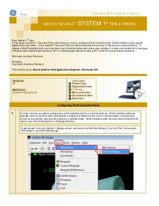
To get started, from your System 1 display screen, we need to set the Data Range. From the “Plot” menu select
“Plot Session” and “Edit Data Range”

2. 2 Configure the data range. For this example we will use “Historical Data” and select the Event Data which
represents the data you wish to use (“Event Data”, “Recent Data Range” or “Fixed Data Range”). We will use “Fixed
Date Range”, but any of the data can be used
3 Next, drill down to the machine you want to create the Shaft Centerline plot for. Drill down to the machine
case, right click on the case either in the machine train view or in the hierarchy. Here we will select the
machine case “HPIP Steam Turbine” so we can generate the shaft centerline plots for both ends of the
machine at once. From the pop up menu select “Plots” and “Shaft Centerline”

3. 4 This will open the Shaft Centerline plot displaying the first of the two bearings we selected in an auto scale
mode. To see the second bearing you can click the right arrow at the bottom of the plot or you can display
both at once by selecting the multi-page view.
5 To adjust the manual scaling, right click on the plot and select “Configure”. This will open the Shaft
Average Centerline Plot Group Configuration dialog screen.

4. 6 Select “Edit Manual Scales”
7 Adjust Plot 1, the first 4 columns are your plot scaling options. Typically these will be set to your bearing
dimensions, assuming all the points of interest are within your bearing clearance.
1) Set Min and Max X to – and + half your bearing’s X diametrical clearance and set Min and Max Y to zero
for the bearing’s Y diametrical clearance.
2) Set the X and Y bearing clearance.
1 2

5. 8 3) Next, set rotor position.
For a typical horizontal machine you would set the position to “Bottom”. This means you expect the
reference data to represent the shaft sitting at the bottom of the bearing clearance. On an overhung rotor
you may anticipate the rotor to start in the top of the bearing on the coupled end. On a vertical machine the
center may be more likely.
Make sure the “Show Clearance Boundaries” is checked.
If the second bearing is the same you can click “Copy” under “Apply to all Plots”
Click “OK” to save your settings.
3
9 Select your reference data. If reference data has not been collected for this bearing the “First Sample” on a
startup or the “Last Sample” on a coast down is a good place to start. — Select “Manual Scale Plots”. —
Select “Apply” and “OK”

6. 1 Once you are happy with your choices don’t forget to save this as a plot session for the next time you want
0 to view these plots.
DID YOU KNOW?
With System1 version 6.81 or newer you can now export timebase waveform data to a .csv file. To do this, open a
timebase or orbit plot. Right click and from the menu select “Export to CSV” and the “To File” or “To Clipboard”
from the sub-menu. It is that simple. You can then open this file in another program such as MS Excel, or another
program that “understands” .csv files.
Bently Nevada Technical Support:
bntechsupport@ge.com
775-215-1818
Bently Nevada website:
http://www.ge-mcs.com/en/bently-nevada.html