Limitation of using black's shortcut to portfolio optimization in excel
•
1 recomendación•941 vistas


Recomendados
Más contenido relacionado
La actualidad más candente
Destacado
Destacado (20)
Similar a Limitation of using black's shortcut to portfolio optimization in excel
Similar a Limitation of using black's shortcut to portfolio optimization in excel (20)
Más de Tai Tran
Más de Tai Tran (20)
Limitation of using black's shortcut to portfolio optimization in excel
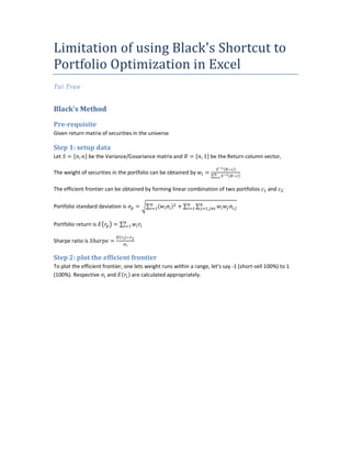
- 1. Limitation of using Black's Shortcut to Portfolio Optimization in Excel Tai Tran Black's Method Pre-requisite Given return matrix of securities in the universe Step 1: setup data Let = , be the Variance/Covariance matrix and = , 1 be the Return column vector, The weight of securities in the portfolio can be obtained by =∑ The efficient frontier can be obtained by forming linear combination of two portfolios and Portfolio standard deviation is = ∑ +∑ ∑ , , Portfolio return is =∑ Sharpe ratio is ℎ = Step 2: plot the efficient frontier To plot the efficient frontier, one lets weight runs within a range, let's say -1 (short-sell 100%) to 1 (100%). Respective and are calculated appropriately.
- 2. The efficient frontier is a scattered plot with as x-axis and as y-axis The optimal portfolio tangent with Capital Market Line is the one with highest Sharpe ratio. That is 1.30872 The issue One issue arises here. The position that produces Sharpe ratio equal 1.30872 may be close, but not exactly the optimal one. The range has a spread (in this case 0.05). If we makes the spread smaller, we may get to a Sharpe ratio even higher than 1.30872 Indeed, at = 0.64, Sharpe ratio hits 1.30873
- 3. The smaller the spread we make, the closer we get to the optimal portfolio. Solution The solution to the issue is to use a solver that would maximize Sharpe ratio, with weights as variables. This way, we utilize Excel's computation power to solve the tangency portfolio problem for us.