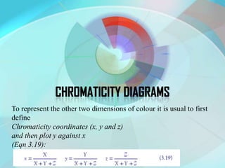
1. To represent the other two dimensions of colour it is usual to first
define
Chromaticity coordinates (x, y and z)
and then plot y against x
(Eqn 3.19):

2. CHROMATICITY DIAGRAM

3. From Eqn 3.19 it follows that
x + y + z = 1 for all colours;
it is therefore only necessary to quote two of the chromaticity
coordinates,
and these can of course be plotted on a normal
two-dimensional graph.
It can also be shown that X and Z can easily be calculated
from x, y and Y;
hence the latter set is an acceptable form of
specification, and consideration of Y values and plots of y
against x should cover all possible colours. A plot of y
against x is called a chromaticity diagram. Such a plot is
shown in Figure 3.7, in which the
spectrum colours are plotted.

4. From Eqn 3.19 it follows
that
x + y + z = 1 for all
colours;
A plot of y against x is
called a chromaticity
diagram.
Such a plot is shown in
Figure 3.7, in which the
spectrum colours are
plotted.

5. From Eqn 3.19 it follows that
x + y + z = 1 for all colours;
The line joining the spectrum
colours is known as the
Spectrum Locus.
The x and y values for each
wavelength were obtained from
the corresponding
distribution coefficients (1931
standard observer in this case)
(Eqn 3.20):

6. where pure colours fall on the chromaticity diagram.
Wavelengths around 480 nm look blue,
wavelengths around 520 nm look green,
while wavelengths from 630 nm to the end of the spectrum look red.
Colours with x and y values close to the spectrum locus
will be very saturated colours
with hues close to those of the corresponding spectrum colours.
For other colours the problem is more difficult.

7. Consequently. in attempting to predict
colour appearance from chromaticity
coordinates or tristimulus values
we must be careful to ascertain
which illuminant has been used.
Strictly speaking, in any application
we should also be careful to ascertain
which standard observer
and which set of observing and viewing conditions are
appropriate,
but these are not normally as important as the illuminant.

8. If we now consider colours
relative only to illuminant C
(surface colours illuminated by illuminant C
and coloured lights with the eye adapted to illuminant C),
the positions for other colours can be deduced from a simple property of the
chromaticity diagram.

9. two points on the chromaticity diagram,
If two coloured lights are represented by
two points on the chromaticity diagram,
then any additive mixture of the two will correspond
to a point on the straight line
joining the two points.
Since the spectrum locus is always concave, it follows that all real
colours
(each of which must correspond to one or more wavelengths
additively mixed)
must fall within the area bounded by the spectrum locus and joining
the ends.
Mixing white light (illuminant C) with monochromatic light of
wavelength 520 nm will give points exactly on the line CG in Figure
3.7.

10. two points on the chromaticity diagram,
Since light of 520 nm looks green, the mixtures will appear various
shades of green, from white through pale greens
to the saturated green of the spectrum colour.
(The points will fall exactly on the line;
the colours seen will not necessarily look exactly the same hue.
What is seen depends on many factors,
but generally mixing white light
and a spectrum colour will produce a
slight but significant change in hue.)

11. two points on the chromaticity diagram,
All colours lying on the line CG
may be described
as colours having a dominant
wavelength of 520 nm.
Similarly mixing white light and
light of wavelength 700 nm (red) will
produce a range of pinks and reds.
In general, the more the colour
resembles the spectrum colour,
the closer will the point be to the
spectrum locus,
while near-neutral colours will
correspond to points close to C.

12. two points on the chromaticity diagram,
For colour F in Figure 3.7 this attribute As the excitation
is defined by purity increases
the colour will
the ratio CF : CG, known as the look less
like a neutral
colour and more
excitation purity of colour F. like the
corresponding
As the excitation purity increases the spectrum
colour.
colour will look less
like a neutral colour and more like
the corresponding spectrum colour.
Samples with excitation purity as
low as 0.1 (or 10%) will look
distinctly different from neutral.
Even very saturated-looking
samples, particularly greens, will have
excitation purities far from 1 (or

13. two points on the chromaticity diagram,
For the sample used as an example for As the excitation
the calculation of tristimulus values purity increases
the colour will
X = 38, look less
like a neutral
Y = 45 and colour and more
Z = 21, like the
corresponding
hence x = 0.365 and y = 0.433. spectrum
colour.
Remembering that the tristimulus
values were calculated for illuminant
A,
we can see that the dominant
wavelength is about 500 nm and
hence the sample is a green-blue

14. two points on the chromaticity diagram,
For the sample used as an example for As the excitation
the calculation of tristimulus values purity increases
the colour will
X = 38, look less
like a neutral
Y = 45 and colour and more
Z = 21, like the
corresponding
hence x = 0.365 and y = 0.433. spectrum
colour.
If, however, the illuminant was
mistakenly taken to be C the
dominant wavelength would have
been estimated to be about 580 nm
and the colour judged to be yellow!

15. Chromaticity diagram
It was stated in section 3.11 that the Y scale is far from uniform. The
same applies to
the xy diagram; equal distances in the diagram do not correspond to
equal visual differences.
For a fixed difference in x and y
the difference seen would be much smaller
for a pair of green samples
than for pairs of blue or grey samples.
It has been emphasised that colour is three-dimensional.
Thus no two-dimensional plot can represent colour completely.
In the case of the chromaticity diagram it is simplest
to regard the missing factor as the Y tristimulus value.

16. two points on the chromaticity diagram,
Consider a sample where R = 10% at all
wavelengths. As the excitation
purity increases
the colour will
look less
If the sample is illuminated by illuminant C the like a neutral
colour and more
tristimulus values are simply like the
one-tenth of the corresponding values for the corresponding
spectrum
sample described in Appendix 3 colour.
 (where R = 100% at all wavelengths)
and the chromaticity coordinates
are the same:
x = 0.310 and y = 0.316.
Both samples are neutral and the difference
between the two is indicated by the Y tristimulus
values. A neutral sample with a Y value of 100
would be white, while one with a Y value of 10
would be a darkish grey.

17. two points on the chromaticity diagram,
All other samples with similar chromaticity coordinates would look
neutral,
but could be white, black or any intermediate shade of grey.
(All samples with constant R values
will look neutral, but the converse does not hold;
many neutral-looking samples have R values that vary considerably
with wavelength.)
Similarly a colour fairly close to neutral but with a dominant
wavelength of 650 nm would look
a pale pink if the Y value was very high (the colour was very light),
but a reddish grey if the Y value was low (the sample was dark).

18. two points on the chromaticity diagram,
In general, any one point on the chromaticity diagram
corresponds to a range of colours differing in lightness,
and this should always be kept in mind
when trying to visualise the colours corresponding to particular chromaticity
coordinates.
The relationships between x, y and Y values
on the one hand and
 the visual appearance on the other
could be developed much further,
but it is recommended that, if possible, students should measure their own
samples.
With modern instruments a student can measure dozens of samples in an hour, and
compare the readings obtained with the visual appearance of the samples.
This is far better than relying on the vague terms such as grey, red, pink and so forth
that have to be used in a textbook. Particular attention should be paid to colours
such as browns, fawns and purples.
After a little practice it is instructive, for each new sample, to estimate the
dominant wavelength, excitation purity, x, y and Y before making measurements.