Partitioning and Positioning (to Solve MINLP Problems) Industrial Modeling Framework (PrPs-IMF)

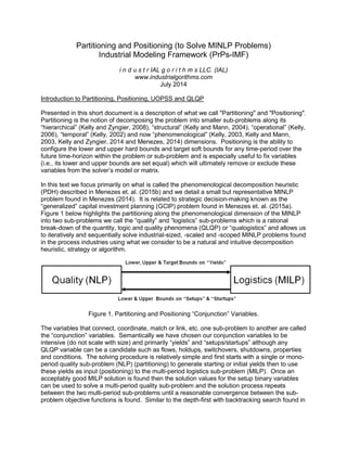
Partitioning and Positioning (to Solve MINLP Problems)
Industrial Modeling Framework (PrPs-IMF)
i n d u s t r IAL g o r i t h m s LLC. (IAL)
www.industrialgorithms.com
July 2014
Introduction to Partitioning, Positioning, UOPSS and QLQP
Presented in this short document is a description of what we call "Partitioning" and "Positioning".
Partitioning is the notion of decomposing the problem into smaller sub-problems along its
“hierarchical” (Kelly and Zyngier, 2008), “structural” (Kelly and Mann, 2004), “operational” (Kelly,
2006), “temporal” (Kelly, 2002) and now “phenomenological” (Kelly, 2003, Kelly and Mann,
2003, Kelly and Zyngier, 2014 and Menezes, 2014) dimensions. Positioning is the ability to
configure the lower and upper hard bounds and target soft bounds for any time-period over the
future time-horizon within the problem or sub-problem and is especially useful to fix variables
(i.e., its lower and upper bounds are set equal) which will ultimately remove or exclude these
variables from the solver’s model or matrix.
In this text we focus primarily on what is called the phenomenological decomposition heuristic
(PDH) described in Menezes et. al. (2015b) and we detail a small but representative MINLP
problem found in Menezes (2014). It is related to strategic decision-making known as the
“generalized” capital investment planning (GCIP) problem found in Menezes et. al. (2015a).
Figure 1 below highlights the partitioning along the phenomenological dimension of the MINLP
into two sub-problems we call the “quality” and “logistics” sub-problems which is a rational
break-down of the quantity, logic and quality phenomena (QLQP) or “qualogistics” and allows us
to iteratively and sequentially solve industrial-sized, -scaled and -scoped MINLP problems found
in the process industries using what we consider to be a natural and intuitive decomposition
heuristic, strategy or algorithm.
Figure 1. Partitioning and Positioning “Conjunction” Variables.
The variables that connect, coordinate, match or link, etc. one sub-problem to another are called
the “conjunction” variables. Semantically we have chosen our conjunction variables to be
intensive (do not scale with size) and primarily “yields” and “setups/startups” although any
QLQP variable can be a candidate such as flows, holdups, switchovers, shutdowns, properties
and conditions. The solving procedure is relatively simple and first starts with a single or mono-
period quality sub-problem (NLP) (partitioning) to generate starting or initial yields then to use
these yields as input (positioning) to the multi-period logistics sub-problem (MILP). Once an
acceptably good MILP solution is found then the solution values for the setup binary variables
can be used to solve a multi-period quality sub-problem and the solution process repeats
between the two multi-period sub-problems until a reasonable convergence between the sub-
problem objective functions is found. Similar to the depth-first with backtracking search found in

Kelly (2002), this same technique can also be employed here whereby each sub-problem, due
to its inherent non-convexity, will mostly likely exhibit multiple local solutions per sub-problem
solve. By retaining then recovering these solutions using unformatted binary files for example
and applying a systematic search mechanism similar to branch-and-bound, multiple solution
paths can be circumscribed where the goal is to find the best overall or combined solution with
the highest profit, best performance and/or least amount of penalties i.e., the combination of
both MILP and NLP sub-problem solutions making up the MINLP problem.
To more effectively articulate the partitioning and positioning concepts, Figure 2 shows the unit-
operation-port-state superstructure (UOPSS) or flowsheet for the previously mentioned MINLP
GCIP problem where the UOPSS shapes can be found in Kelly (2004), Kelly (2005), Zyngier
and Kelly (2009) and Zyngier and Kelly (2012).
Figure 2. Partitioning and Positioning GCIP Example UOPSS Flowsheet.

This problem is formulated whereby both the capacity and capital cost for the expansion and
installation of the Diesel Hydro-Treating units (DHT1 and DHT2 respectively) are modeled as
“flows”. Diamond shapes are perimeters which indicate where material or even money and
other necessary resources can flow into or out of the problem. We have a supply of D1000
which has a diesel sulfur content or concentration in weight percent of 0.1000 (1000 wppm), a
demand of D50 (0.0050 wt%) and D15 (0.0015 wt%) and a production of wild naphtha (WN)
which is a by-product of the desulfurization process. There is no explicit consumption of
hydrogen shown given that it is not perceived as a bottleneck or active constraint. The square
shapes with an “x” through them are continuous-processes and the triangle shapes are pools or
inventory/storage unit-operations. The circles are ports where an “x” inside is an out-port and
without an “x” is in-port and the lines connected to ports and units are what we call “internal
streams”. Lines with arrow-heads connecting out-ports to in-ports are called “external streams”
and these along with the unit-operations have setup and startup logic variables created as well
as switchovers and shutdown logic variables if up-times and/or down-times are configured to
manage the temporal transitions (Kelly and Zyngier, 2007 and Zyngier and Kelly, 2009).
The scope of this problem is to decide if the existing unit DHT1 should be expanded via the
commission-stage operation or not and to decide if the non-existing unit DHT2 should be
installed via the construction-stage operation or not. If so then there is a capital cost during the
commission and construction-stages for the capacity expansion and installation using a variable
and fixed cost linear expression of:
capital cost = alpha * (capacity_new – capacity_old) + beta * setup
where if an installation, the old capacity is of course 0 (zero). A more detailed description of this
problem can be found in GCIP-SDSU-IMF.docx (IAL, June, 2014). There is a severity condition
that provides the degree of hydro-desulfurization which manipulates or controls the yields and
sulfur concentrations on out-ports “o” and “o2” for both DHT1 and DHT2 as the following
formulas:
yield,o = 1.0 - (severity - 0.90) / 2.0
yield,o2 = (severity - 0.90) / 2.0
and
sulfur,o = (1.0 – severity) * sulfur,i
where sulfur,i is the sulfur content on the in-ports to the hydro-treaters. The density SG is
required to perform the mass-basis sulfur balances. There is no cost applied to the supply of
diesel nor is there a price for wild naphtha. However, the D50 product has a price of 1.0 and the
price for D15 is 1.2 which implies that it is more economical to produce a lower sulfur diesel
material especially when there is no raw material or operating costs currently modeled.
As mentioned, this problem is a MINLP problem given that all flows are variable as well as the
specific-gravities and sulfur concentrations including the severity times sulfur thus resulting in bi-
linear and tri-linear terms with plus and minus coefficients making the NLP quality sub-problem
non-convex. Due to the setup logic variables for the expansion and/or installation logic
decisions we have the integer or discrete (binary) variables resulting in the MINLP and more
appropriately a non-convex MINLP problem.
Industrial Modeling Framework (IMF), IMPL and SIIMPLE

To implement the mathematical formulation of this and other systems, IAL offers a unique
approach and is incorporated into our Industrial Modeling Programming Language we call IMPL.
IMPL has its own modeling language called IML (short for Industrial Modeling Language) which
is a flat or text-file interface as well as a set of API's which can be called from any computer
programming language such as C, C++, Fortran, C#, VBA, Java (SWIG), Python (CTYPES)
and/or Julia (CCALL) called IPL (short for Industrial Programming Language) to both build the
model and to view the solution. Models can be a mix of linear, mixed-integer and nonlinear
variables and constraints and are solved using a combination of LP, QP, MILP and NLP solvers
such as COINMP, GLPK, LPSOLVE, SCIP, CPLEX, GUROBI, LINDO, XPRESS, CONOPT,
IPOPT, KNITRO and WORHP as well as our own implementation of SLP called SLPQPE
(Successive Linear & Quadratic Programming Engine) which is a very competitive alternative to
the other nonlinear solvers and embeds all available LP and QP solvers.
In addition and specific to DRR problems, we also have a special solver called SECQPE
standing for Sequential Equality-Constrained QP Engine which computes the least-squares
solution and a post-solver called SORVE standing for Supplemental Observability, Redundancy
and Variability Estimator to estimate the usual DRR statistics. SECQPE also includes a
Levenberg-Marquardt regularization method for nonlinear data regression problems and can be
presolved using SLPQPE i.e., SLPQPE warm-starts SECQPE. SORVE is run after the
SECQPE solver and also computes the well-known "maximum-power" gross-error statistics
(measurement and nodal/constraint tests) to help locate outliers, defects and/or faults i.e., mal-
functions in the measurement system and mis-specifications in the logging system.
The underlying system architecture of IMPL is called SIIMPLE (we hope literally) which is short
for Server, Interfacer (IML), Interacter (IPL), Modeler, Presolver Libraries and Executable. The
Server, Presolver and Executable are primarily model or problem-independent whereas the
Interfacer, Interacter and Modeler are typically domain-specific i.e., model or problem-
dependent. Fortunately, for most industrial planning, scheduling, optimization, control and
monitoring problems found in the process industries, IMPL's standard Interfacer, Interacter and
Modeler are well-suited and comprehensive to model the most difficult of production and
process complexities allowing for the formulations of straightforward coefficient equations,
ubiquitous conservation laws, rigorous constitutive relations, empirical correlative expressions
and other necessary side constraints.
User, custom, adhoc or external constraints can be augmented or appended to IMPL when
necessary in several ways. For MILP or logistics problems we offer user-defined constraints
configurable from the IML file or the IPL code where the variables and constraints are
referenced using unit-operation-port-state names and the quantity-logic variable types. It is also
possible to import a foreign *.ILP file (row-based MPS file) which can be generated by any
algebraic modeling language or matrix generator. This file is read just prior to generating the
matrix and before exporting to the LP, QP or MILP solver. For NLP or quality problems we offer
user-defined formula configuration in the IML file and single-value and multi-value function
blocks writable in C, C++ or Fortran. The nonlinear formulas may include intrinsic functions
such as EXP, LN, LOG, SIN, COS, TAN, MIN, MAX, IF, NOT, EQ, NE, LE, LT, GE, GT and CIP,
LIP, SIP and KIP (constant, linear and monotonic spline interpolations) as well as user-written
extrinsic functions (XFCN). It is also possible to import another type of foreign file called the
*.INL file where both linear and nonlinear constraints can be added easily using new or existing
IMPL variables.
Industrial modeling frameworks or IMF's are intended to provide a jump-start to an industrial
project implementation i.e., a pre-project if you will, whereby pre-configured IML files and/or IPL

code are available specific to your problem at hand. The IML files and/or IPL code can be
easily enhanced, extended, customized, modified, etc. to meet the diverse needs of your project
and as it evolves over time and use. IMF's also provide graphical user interface prototypes for
drawing the flowsheet as in Figure 1 and typical Gantt charts and trend plots to view the solution
of quantity, logic and quality time-profiles. Current developments use Python 2.3 and 2.7
integrated with open-source Dia and Matplotlib modules respectively but other prototypes
embedded within Microsoft Excel/VBA for example can be created in a straightforward manner.
However, the primary purpose of the IMF's is to provide a timely, cost-effective, manageable
and maintainable deployment of IMPL to formulate and optimize complex industrial
manufacturing systems in either off-line or on-line environments. Using IMPL alone would be
somewhat similar (but not as bad) to learning the syntax and semantics of an AML as well as
having to code all of the necessary mathematical representations of the problem including the
details of digitizing your data into time-points and periods, demarcating past, present and future
time-horizons, defining sets, index-sets, compound-sets to traverse the network or topology,
calculating independent and dependent parameters to be used as coefficients and bounds and
finally creating all of the necessary variables and constraints to model the complex details of
logistics and quality industrial optimization problems. Instead, IMF's and IMPL provide, in our
opinion, a more elegant and structured approach to industrial modeling and solving so that you
can capture the benefits of advanced decision-making faster, better and cheaper.
Partitioning and Positioning Synopsis
At this point we explore further the purpose and procedure of partitioning and positioning in
terms of its usefulness in advanced planning and scheduling applications. Appendix A records
the UOPSS superstructure or flowsheet shapes for the GCIP example problem in the UPS file.
Appendices B, C and D contain the IML configurations for the starting “NLPT1” using only one
time-period, the “MILPT3” three-period logistics sub-problem and the “NLPT3” three-period
quality sub-problem respectively.
There is a another file called the OML (Output Model Language) file which is used to tell IMPL
which UOPSS, QLQP variables and in which time-periods they are to be outputted. This is
useful to allow ad hoc export of any variable’s address, index or pointer using the (UOPSS,
QLQP, T) (place, property, period) coordinates. The QLQP attributes are specified using the
keywords: FL (flow), HU (holdup), YD (yield), SP (setup), SU (startup), SV (switchover-to-itself),
DN (density), CM (component), PR (property), CN (condition) and CO (coefficient). A user “tag”
string is also provided to identify, reference, name or label the variable’s solution value in the
specified output file (usually a data CSV flat-file) and this can be used as a “calc” or calculation
name in IML (notice the “&sCalc,@rValue” header and footer in the OML files). We use the
output data CSV files as input from one sub-problem solution to the next sub-problem and this
provides the positioning or coordination between the partitions or sub-problems i.e., NLPT1.DAT
(fixed/finite yields) -> MILPT3.IML, MILPT3.DAT (fixed setups) -> NLPT3.IML and NLPT3.DAT
(fixed/finite yields) -> MILPT3.IML. It should be noted that in the MILPT3.IML file, it inputs both
the NLPT1.DAT and NLPT3.DAT in order to ensure that there is at least a non-zero default yield
value given that if a unit-operation is not setup in a particulate time-period then it will have a
yield of zero (0) given the semi-continuous found in our IMPL Modeler. If the yield found from
NLPT3 is zero (0) then the default from NLPT1 is used instead.
When we solve the NLPT1 (temporal relaxation) sub-problem using SLPQPE, with either
COINMP, GLPK or LPSOLVE as the LP solvers, we get an objective function value of 0.975
currency-units given that we have only allowed the existing DHT1 and non-existing DHT2 unit-

operations to be active during the mono-period time-horizon in order to provide starting, initial or
default yields to the MILPT3 i.e., no capital costs incurred. The 0.975 value corresponds to the
fact that only flow from the DHT1,Existing,o out-port to the D50,i in-port is active in the amount
of 0.975 flow-units. Upon solving the MIPLT3 using COINMP, GLPK or LPSOLVE we get an
objective function value of 5.638 currency-units which corresponds to the profit of performing
the DHT1 commission-stage in time-period 1 and DHT2 construction-stage also in time-period
1. This allows two (2) time-periods for expanded capacity for DHT1 and also two (2) time-
periods for newly installed and extended capacity and capability for DHT2 i.e., the DHT2 unit
can produce both D50 and D15 due to its extended conversion. The Gantt chart in Figure 3
displays the setup logic variables in black horizontal bars for all unit-operations.
Figure 3. Gantt Chart with 1-period and 3-period Past and Future Horizons for MILPT3.
Using the fixed setups from MILPT3.DAT for both the unit-operations and the unit-operation-
port-state to unit-operation-port-state external streams, we get a profit of 5.647 currency-units
from the NLPT3 sub-problem solution. Solving again the MILPT3 with the new fixed/finite yields
from NLPT3.DAT we converge on an objective function value of 5.647.
In summary, we have described how to use IMPL with IML and OML files to iteratively solve a
qualogistics or MINLP “generalized” capital investment problem (GCIP) using MILP and NLP
sub-solvers configured in a coordinated manner where a more automated integration can be
performed using our IPL coded in a computer programming language. This same technique
can be applied to any advanced planning and scheduling MINLP problem found in the process
industries given our assertion that these types of problems can be structurally and operationally
modeled using our UOPSS flowsheet, phenomenologically modeled using our QLQP attributes
and temporally modeled using our discrete-time and distributed-time digitization where
“conjunction” variables can be employed to concatenate the sub-problems. The major
advantage of our “partitioning” and “positioning” approach is that each sub-problem can be
independently and individually isolated and thoroughly investigated and interrogated to
troubleshoot and debug inconsistencies and unexpected solutions when they exist. Existing
MINLP and Global Optimizers (GO) are treated as black-boxes and if reliable and relevant

solutions are not obtained which is usually the case in practice, then little insight and analysis is
afforded back to the development and/or deployment user.
References
Kelly, J.D., “Chronological decomposition heuristic for scheduling: a divide and conquer
method”, American Institute of Chemical Engineering Journal, 48, (2002).
Kelly, J.D., “Next generation refinery scheduling technology”, NPRA Plant Automation
and Decision Support, San Antonio, USA, September, (2003).
Kelly, J.D., Mann, J.L., “Crude-oil blend scheduling optimization: an application with
multi-million dollar benefits”, Hydrocarbon Processing, June/July, (2003).
Kelly, J.D., Mann, J.L., “Flowsheet decomposition heuristic applied to scheduling: a
relax and fix method”, Computers & Chemical Engineering, 28, (2004).
Kelly, J.D., "Production modeling for multimodal operations", Chemical Engineering Progress,
February, 44, (2004).
Kelly, J.D., "The unit-operation-stock superstructure (UOSS) and the quantity-logic-quality
paradigm (QLQP) for production scheduling in the process industries", In: MISTA 2005
Conference Proceedings, 327, (2005).
Kelly, J.D., “Stock decomposition heuristic for scheduling: a priority and dispatch rule
approach”, Internal Technical Report, (2006).
Kelly, J.D., Zyngier, D., "An improved MILP modeling of sequence-dependent switchovers for
discrete-time scheduling problems", Industrial & Engineering Chemistry Research, 46, 4964,
(2007).
Kelly, J.D., Zyngier, D., “Hierarchical decomposition heuristic for scheduling:
coordinated reasoning for decentralized and distributed decision making problems”,
Computers & Chemical Engineering, 32, (2008).
Zyngier, D., Kelly, J.D., "Multi-product inventory logistics modeling in the process industries", In:
W. Chaovalitwonse, K.C. Furman and P.M. Pardalos, Eds., Optimization and Logistics
Challenges in the Enterprise", Springer, 61-95, (2009).
Zyngier, D., Kelly, J.D., "UOPSS: a new paradigm for modeling production planning and
scheduling systems", ESCAPE 22, June, (2012).
Industrial Algorithms, LLC (IAL), “Generalized Capital Investment Planning w/ Sequence-
Dependent Setups IMF (GCIP-SDSU-IMF.docx)”, June, (2014).
Kelly, J.D., and Zyngier, D., “Unit operation nonlinear modeling for planning and
scheduling applications”, K.C. Furman et. al. (eds.), Optimization and Analytics in the
Oil & Gas Industries, Springer Science, 2014 (accepted).

Menezes, B.C., “Quantitative methods for strategic investment planning in the oil-
refining industry”, PhD Thesis, Federal University of Rio de Janeiro (UFRJ), August,
(2014).
Menezes, B.C., Kelly, J.D., Grossmann, I.E., Vazacopoulos, A., “Generalized capital
investment planning of oil refinery units using MILP and sequence-dependent setups”,
submitted to Computers & Chemical Engineering, (2015a).
Menezes, B.C., Kelly, J.D., Grossmann, I.E., Moro, L.F.L., “Phenomenological
decomposition heuristic for process design synthesis of oil-refinery units”, submitted to
Computers & Chemical Engineering, (2015b).
Appendix A - PartitioningPositioning-IMF.UPS File
i M P l (c)
Copyright and Property of i n d u s t r I A L g o r i t h m s LLC.
checksum,184
!!!!!!!!!!!!!!!!!!!!!!!!!!!!!!!!!!!!!!!!!!!!!!!!!!!!!!!!!!!!!!
! Unit-Operation-Port-State-Superstructure (UOPSS) *.UPS File.
! (This file is automatically generated from the Python program IALConstructer.py)
!!!!!!!!!!!!!!!!!!!!!!!!!!!!!!!!!!!!!!!!!!!!!!!!!!!!!!!!!!!!!!
&sUnit,&sOperation,@sType,@sSubtype,@sUse
Capacity1,,pool,,
Capacity2,,pool,,
Capital,Cost,perimeter,,
Charge1,,processc,,
Charge2,,processc,,
D1000,,perimeter,,
D15,,perimeter,,
D50,,perimeter,,
DHT1,Commission,processc,,
DHT1,Existing,processc,,
DHT1,Expanded,processc,,
DHT2,Construction,processc,,
DHT2,Installed,processc,,
DHT2,NonExisting,processc,,
WN,,perimeter,,
&sUnit,&sOperation,@sType,@sSubtype,@sUse
! Number of UO shapes = 15
&sAlias,&sUnit,&sOperation
ALLPARTS,Capacity1,
ALLPARTS,Capacity2,
ALLPARTS,Capital,Cost
ALLPARTS,Charge1,
ALLPARTS,Charge2,
ALLPARTS,D1000,
ALLPARTS,D15,
ALLPARTS,D50,
ALLPARTS,DHT1,Commission
ALLPARTS,DHT1,Existing
ALLPARTS,DHT1,Expanded
ALLPARTS,DHT2,Construction
ALLPARTS,DHT2,Installed
ALLPARTS,DHT2,NonExisting
ALLPARTS,WN,
&sAlias,&sUnit,&sOperation
&sUnit,&sOperation,&sPort,&sState,@sType,@sSubtype
Capacity1,,i,,in,
Capacity1,,o,,out,
Capacity2,,i,,in,
Capacity2,,o,,out,
Capital,Cost,cpl,,in,
Charge1,,cpl,,out,
Charge1,,cpt,,out,
Charge1,,i,,in,
Charge2,,cpl,,out,
Charge2,,cpt,,out,
Charge2,,i,,in,
D1000,,o,,out,
D15,,i,,in,
D50,,i,,in,
DHT1,Commission,cpt,,out,
DHT1,Commission,i,,in,
DHT1,Commission,o,,out,
DHT1,Commission,o2,,out,

DHT1,Existing,i,,in,
DHT1,Existing,o,,out,
DHT1,Existing,o2,,out,
DHT1,Expanded,cpt,,in,
DHT1,Expanded,i,,in,
DHT1,Expanded,o,,out,
DHT1,Expanded,o2,,out,
DHT2,Construction,cpt,,out,
DHT2,Construction,i,,in,
DHT2,Construction,o,,out,
DHT2,Construction,o2,,out,
DHT2,Installed,cpt,,in,
DHT2,Installed,i,,in,
DHT2,Installed,o,,out,
DHT2,Installed,o2,,out,
DHT2,NonExisting,i,,in,
DHT2,NonExisting,o,,out,
DHT2,NonExisting,o2,,out,
WN,,i,,in,
&sUnit,&sOperation,&sPort,&sState,@sType,@sSubtype
! Number of UOPS shapes = 37
&sAlias,&sUnit,&sOperation,&sPort,&sState
ALLINPORTS,Capacity1,,i,
ALLINPORTS,Capacity2,,i,
ALLINPORTS,Capital,Cost,cpl,
ALLINPORTS,Charge1,,i,
ALLINPORTS,Charge2,,i,
ALLINPORTS,D15,,i,
ALLINPORTS,D50,,i,
ALLINPORTS,DHT1,Commission,i,
ALLINPORTS,DHT1,Existing,i,
ALLINPORTS,DHT1,Expanded,cpt,
ALLINPORTS,DHT1,Expanded,i,
ALLINPORTS,DHT2,Construction,i,
ALLINPORTS,DHT2,Installed,cpt,
ALLINPORTS,DHT2,Installed,i,
ALLINPORTS,DHT2,NonExisting,i,
ALLINPORTS,WN,,i,
ALLOUTPORTS,Capacity1,,o,
ALLOUTPORTS,Capacity2,,o,
ALLOUTPORTS,Charge1,,cpl,
ALLOUTPORTS,Charge1,,cpt,
ALLOUTPORTS,Charge2,,cpl,
ALLOUTPORTS,Charge2,,cpt,
ALLOUTPORTS,D1000,,o,
ALLOUTPORTS,DHT1,Commission,cpt,
ALLOUTPORTS,DHT1,Commission,o,
ALLOUTPORTS,DHT1,Commission,o2,
ALLOUTPORTS,DHT1,Existing,o,
ALLOUTPORTS,DHT1,Existing,o2,
ALLOUTPORTS,DHT1,Expanded,o,
ALLOUTPORTS,DHT1,Expanded,o2,
ALLOUTPORTS,DHT2,Construction,cpt,
ALLOUTPORTS,DHT2,Construction,o,
ALLOUTPORTS,DHT2,Construction,o2,
ALLOUTPORTS,DHT2,Installed,o,
ALLOUTPORTS,DHT2,Installed,o2,
ALLOUTPORTS,DHT2,NonExisting,o,
ALLOUTPORTS,DHT2,NonExisting,o2,
&sAlias,&sUnit,&sOperation,&sPort,&sState
&sUnit,&sOperation,&sPort,&sState,&sUnit,&sOperation,&sPort,&sState
Capacity1,,o,,DHT1,Expanded,cpt,
Capacity2,,o,,DHT2,Installed,cpt,
Charge1,,cpl,,Capital,Cost,cpl,
Charge1,,cpt,,Capacity1,,i,
D1000,,o,,DHT1,Commission,i,
D1000,,o,,DHT1,Existing,i,
D1000,,o,,DHT1,Expanded,i,
D1000,,o,,DHT2,Construction,i,
D1000,,o,,DHT2,Installed,i,
D1000,,o,,DHT2,NonExisting,i,
DHT1,Commission,cpt,,Charge1,,i,
DHT1,Commission,o,,D50,,i,
DHT1,Commission,o2,,WN,,i,
DHT1,Existing,o,,D50,,i,
DHT1,Existing,o2,,WN,,i,
DHT1,Expanded,o,,D50,,i,
DHT1,Expanded,o2,,WN,,i,
DHT2,Construction,cpt,,Charge2,,i,
DHT2,Construction,o,,D15,,i,
DHT2,Construction,o2,,WN,,i,
DHT2,Installed,o,,D15,,i,
DHT2,Installed,o2,,WN,,i,
DHT2,NonExisting,o,,D15,,i,
DHT2,NonExisting,o2,,WN,,i,
&sUnit,&sOperation,&sPort,&sState,&sUnit,&sOperation,&sPort,&sState

! Number of UOPSPSUO shapes = 29
!&sUnit,&sOperation,&sPort,&sState,&sUnit,&sOperation,&sPort,&sState
DHT1,Commission,cpt,,Charge1,,i,
DHT2,Construction,cpt,,Charge2,,i,
DHT1,Commission,o,,D50,,i,
DHT1,Existing,o,,D50,,i,
DHT1,Expanded,o,,D50,,i,
D1000,,o,,DHT1,Commission,i,
D1000,,o,,DHT1,Existing,i,
Capacity1,,o,,DHT1,Expanded,cpt,
D1000,,o,,DHT1,Expanded,i,
D1000,,o,,DHT2,Construction,i,
Capacity2,,o,,DHT2,Installed,cpt,
D1000,,o,,DHT2,Installed,i,
D1000,,o,,DHT2,NonExisting,i,
DHT1,Commission,o2,,WN,,i,
DHT1,Existing,o2,,WN,,i,
DHT1,Expanded,o2,,WN,,i,
DHT2,Construction,o2,,WN,,i,
DHT2,Installed,o2,,WN,,i,
DHT2,NonExisting,o2,,WN,,i,
!&sUnit,&sOperation,&sPort,&sState,&sUnit,&sOperation,&sPort,&sState
&sAlias,&sUnit,&sOperation,&sPort,&sState,&sUnit,&sOperation,&sPort,&sState
ALLPATHS,Charge1,,cpt,,Capacity1,,i,
ALLPATHS,Charge2,,cpt,,Capacity2,,i,
ALLPATHS,Charge1,,cpl,,Capital,Cost,cpl,
ALLPATHS,Charge2,,cpl,,Capital,Cost,cpl,
ALLPATHS,DHT1,Commission,cpt,,Charge1,,i,
ALLPATHS,DHT2,Construction,cpt,,Charge2,,i,
ALLPATHS,DHT2,Construction,o,,D15,,i,
ALLPATHS,DHT2,Installed,o,,D15,,i,
ALLPATHS,DHT2,NonExisting,o,,D15,,i,
ALLPATHS,DHT1,Commission,o,,D50,,i,
ALLPATHS,DHT1,Existing,o,,D50,,i,
ALLPATHS,DHT1,Expanded,o,,D50,,i,
ALLPATHS,DHT2,Construction,o,,D50,,i,
ALLPATHS,DHT2,Installed,o,,D50,,i,
ALLPATHS,DHT2,NonExisting,o,,D50,,i,
ALLPATHS,D1000,,o,,DHT1,Commission,i,
ALLPATHS,D1000,,o,,DHT1,Existing,i,
ALLPATHS,Capacity1,,o,,DHT1,Expanded,cpt,
ALLPATHS,D1000,,o,,DHT1,Expanded,i,
ALLPATHS,D1000,,o,,DHT2,Construction,i,
ALLPATHS,Capacity2,,o,,DHT2,Installed,cpt,
ALLPATHS,D1000,,o,,DHT2,Installed,i,
ALLPATHS,D1000,,o,,DHT2,NonExisting,i,
ALLPATHS,DHT1,Commission,o2,,WN,,i,
ALLPATHS,DHT1,Existing,o2,,WN,,i,
ALLPATHS,DHT1,Expanded,o2,,WN,,i,
ALLPATHS,DHT2,Construction,o2,,WN,,i,
ALLPATHS,DHT2,Installed,o2,,WN,,i,
ALLPATHS,DHT2,NonExisting,o2,,WN,,i,
&sAlias,&sUnit,&sOperation,&sPort,&sState,&sUnit,&sOperation,&sPort,&sState
Appendix B - PartitioningPositioning-IMF-NLPT1.IML and OML Files
i M P l (c)
!!!!!!!!!!!!!!!!!!!!!!!!!!!!!!!!!!!!!!!!!!!!!!!!!!!!!!!!!!!!!!!!!!!!!!!!!!!!!!!!
! Calculation Data (Parameters)
!!!!!!!!!!!!!!!!!!!!!!!!!!!!!!!!!!!!!!!!!!!!!!!!!!!!!!!!!!!!!!!!!!!!!!!!!!!!!!!!
&sCalc,@sValue
START,-1.0
BEGIN,0.0
END,1.0
PERIOD,1.0
SMALL,0.001
LARGE,10000.0
OLDCAPACITY,1.0
NEWCAPACITY,1.5
EXPAND,0.6
ALPHA_1,0.5
BETA_1,0.5

ALPHA_2,0.5
BETA_2,0.5
&sCalc,@sValue
!!!!!!!!!!!!!!!!!!!!!!!!!!!!!!!!!!!!!!!!!!!!!!!!!!!!!!!!!!!!!!!!!!!!!!!!!!!!!!!!
! Chronological Data (Periods)
!!!!!!!!!!!!!!!!!!!!!!!!!!!!!!!!!!!!!!!!!!!!!!!!!!!!!!!!!!!!!!!!!!!!!!!!!!!!!!!!
@rPastTHD,@rFutureTHD,@rTPD
START,END,PERIOD
!!!!!!!!!!!!!!!!!!!!!!!!!!!!!!!!!!!!!!!!!!!!!!!!!!!!!!!!!!!!!!!!!!!!!!!!!!!!!!!!
! Construction Data (Pointers)
!!!!!!!!!!!!!!!!!!!!!!!!!!!!!!!!!!!!!!!!!!!!!!!!!!!!!!!!!!!!!!!!!!!!!!!!!!!!!!!!
Include-@sFile_Name
PartitioningPositioning-IMF.ups
Include-@sFile_Name
!!!!!!!!!!!!!!!!!!!!!!!!!!!!!!!!!!!!!!!!!!!!!!!!!!!!!!!!!!!!!!!!!!!!!!!!!!!!!!!!
! Capacity Data (Prototypes)
!!!!!!!!!!!!!!!!!!!!!!!!!!!!!!!!!!!!!!!!!!!!!!!!!!!!!!!!!!!!!!!!!!!!!!!!!!!!!!!!
&sUnit,&sOperation,@rRate_Lower,@rRate_Upper
DHT1,Existing,0.0,OLDCAPACITY
DHT1,Commission,0.0,0.0
DHT1,Expanded,0.0,0.0
DHT2,NonExisting,0.0,SMALL
DHT2,Construction,0.0,0.0
DHT2,Installed,0.0,0.0
Charge1,,0.0,0.0
Charge2,,0.0,0.0
&sUnit,&sOperation,@rHoldup_Lower,@rHoldup_Upper
Capacity1,,0.0,NEWCAPACITY*END
&sUnit,&sOperation,&sPort,&sState,@rTotalRate_Lower,@rTotalRate_Upper
ALLINPORTS,0.0,LARGE
ALLOUTPORTS,0.0,LARGE
&sUnit,&sOperation,&sPort,&sState,@rTeeRate_Lower,@rTeeRate_Upper
DHT1,Expanded,cpt,,0.0,NEWCAPACITY
DHT2,Installed,cpt,,0.0,NEWCAPACITY
&sUnit,&sOperation,&sPort,&sState,@rYield_Lower,@rYield_Upper,@rYield_Fixed
DHT1,Existing,i,,1.0,1.0,
DHT1,Existing,o,,0.0,1.0,
DHT1,Existing,o2,,0.0,1.0,
DHT1,Commission,i,,1.0,1.0,
DHT1,Commission,o,,0.0,1.0,
DHT1,Commission,o2,,0.0,1.0,
DHT1,Commission,cpt,,0.0,LARGE,
DHT1,Expanded,i,,1.0,1.0,
DHT1,Expanded,o,,0.0,1.0,
DHT1,Expanded,o2,,0.0,1.0,
DHT1,Expanded,cpt,,1.0,LARGE,
DHT2,NonExisting,i,,1.0,1.0,
DHT2,NonExisting,o,,0.0,1.0,
DHT2,NonExisting,o2,,0.0,1.0,
DHT2,Construction,i,,1.0,1.0,
DHT2,Construction,o,,0.0,1.0,
DHT2,Construction,o2,,0.0,1.0,
DHT2,Construction,cpt,,0.0,LARGE,
DHT2,Installed,i,,1.0,1.0,
DHT2,Installed,o,,0.0,1.0,
DHT2,Installed,o2,,0.0,1.0,
DHT2,Installed,cpt,,1.0,LARGE,
Charge1,,i,,1.0,1.0
Charge1,,cpl,,EXPAND*ALPHA_1,EXPAND*ALPHA_1,EXPAND*(BETA_1-ALPHA_1*OLDCAPACITY)
Charge1,,cpt,,0.0,0.0
Charge2,,i,,1.0,1.0
Charge2,,cpl,,ALPHA_2,ALPHA_2,BETA_2
!!!!!!!!!!!!!!!!!!!!!!!!!!!!!!!!!!!!!!!!!!!!!!!!!!!!!!!!!!!!!!!!!!!!!!!!!!!!!!!!

! Constituent Data (Properties)
!!!!!!!!!!!!!!!!!!!!!!!!!!!!!!!!!!!!!!!!!!!!!!!!!!!!!!!!!!!!!!!!!!!!!!!!!!!!!!!!
&sDensity
SG
&sDensity
&sProperty
S
&sProperty
&sProperty,@sDensity
S,SG
&sUnit,&sOperation,&sPort,&sState,&sDensity,@rDensity_Lower,@rDensity_Upper,@rDensity_Target
ALLINPORTS,SG,0.0,2.0,
ALLOUTPORTS,SG,0.0,2.0,
D1000,,o,,SG,0.82,0.82
&sUnit,&sOperation,&sPort,&sState,&sProperty,@rProperty_Lower,@rProperty_Upper,@rProperty_Target
ALLINPORTS,S,0.0,1.0,
ALLOUTPORTS,S,0.0,1.0,
D1000,,o,,S,0.1,0.1
&sCondition
SG
S
SEV
&sCondition
&sUnit,&sOperation,&sCondition,@rCondition_Lower,@rCondition_Upper,@rCondition_Target
DHT1,Existing,SG,0.8,2.0,
DHT1,Existing,S,0.000,1.0,
DHT1,Existing,SEV,0.90,0.95,
DHT1,Commission,SG,0.8,2.0,
DHT1,Commission,S,0.000,1.0,
DHT1,Commission,SEV,0.90,0.95,
DHT1,Expanded,SG,0.8,2.0,
DHT1,Expanded,S,0.000,1.0,
DHT1,Expanded,SEV,0.90,0.95,
DHT2,NonExisting,SEV,0.90,0.99,
DHT2,NonExisting,SG,0.8,2.0,
DHT2,NonExisting,S,0.0,1.0,
DHT2,Construction,SEV,0.90,0.99,
DHT2,Construction,SG,0.8,2.0,
DHT2,Construction,S,0.0,1.0,
DHT2,Installed,SEV,0.90,0.99,
DHT2,Installed,SG,0.8,2.0,
DHT2,Installed,S,0.0,1.0,
UOPSDensityUOCondition-&sUnit,&sOperation,&sPort,&sState,&sDensity,&sUnit,&sOperation,&sCondition
DHT1,Existing,i,,SG,DHT1,Existing,SG
DHT1,Commission,i,,SG,DHT1,Commission,SG
DHT1,Expanded,i,,SG,DHT1,Expanded,SG
DHT2,NonExisting,i,,SG,DHT2,NonExisting,SG
DHT2,Construction,i,,SG,DHT2,Construction,SG
DHT2,Installed,i,,SG,DHT2,Installed,SG
UOPSPropertyUOCondition-&sUnit,&sOperation,&sPort,&sState,&sProperty,&sUnit,&sOperation,&sCondition
DHT1,Existing,i,,S,DHT1,Existing,S
DHT1,Commission,i,,S,DHT1,Commission,S
DHT1,Expanded,i,,S,DHT1,Expanded,S
DHT2,NonExisting,i,,S,DHT2,NonExisting,S
DHT2,Construction,i,,S,DHT2,Construction,S
DHT2,Installed,i,,S,DHT2,Installed,S
ConditionsUOPSYield-&sUnit,&sOperation,&sPort,&sState,@sType,@rValue,@sValue
DHT1,Existing,o,,?,3,(1.0- (SEV-0.90)/2)
DHT1,Commission,o,,?,3,(1.0- (SEV-0.90)/2)
DHT1,Expanded,o,,?,3,(1.0- (SEV-0.90)/2)
DHT1,Existing,o2,,?,3, (SEV-0.90)/2
DHT1,Commission,o2,,?,3, (SEV-0.90)/2
DHT1,Expanded,o2,,?,3, (SEV-0.90)/2
DHT2,NonExisting,o,,?,3,(1.0- (SEV-0.90)/2)
DHT2,Construction,o,,?,3,(1.0- (SEV-0.90)/2)
DHT2,Installed,o,,?,3,(1.0- (SEV-0.90)/2)
DHT2,NonExisting,o2,,?,3, (SEV-0.90)/2
DHT2,Construction,o2,,?,3, (SEV-0.90)/2
DHT2,Installed,o2,,?,3, (SEV-0.90)/2
ConditionsUOPSDensity-&sUnit,&sOperation,&sPort,&sState,&sDensity,@sType,@rValue,@sValue
DHT1,Existing,o,,SG,?,3,SG

DHT1,Commission,o,,SG,?,3,SG
DHT1,Expanded,o,,SG,?,3,SG
DHT2,NonExisting,o,,SG,?,3,SG
DHT2,Construction,o,,SG,?,3,SG
DHT2,Installed,o,,SG,?,3,SG
ConditionsUOPSProperty-&sUnit,&sOperation,&sPort,&sState,&sProperty,@sType,@rValue,@sValue
DHT1,Existing,o,,S,?,3,(1.0-SEV)*S
DHT1,Commission,o,,S,?,3,(1.0-SEV)*S
DHT1,Expanded,o,,S,?,3,(1.0-SEV)*S
DHT2,NonExisting,o,,S,?,3,(1.0-SEV)*S
DHT2,Construction,o,,S,?,3,(1.0-SEV)*S
DHT2,Installed,o,,S,?,3,(1.0-SEV)*S
!!!!!!!!!!!!!!!!!!!!!!!!!!!!!!!!!!!!!!!!!!!!!!!!!!!!!!!!!!!!!!!!!!!!!!!!!!!!!!!!
! Cost Data (Pricing)
!!!!!!!!!!!!!!!!!!!!!!!!!!!!!!!!!!!!!!!!!!!!!!!!!!!!!!!!!!!!!!!!!!!!!!!!!!!!!!!!
&sUnit,&sOperation,&sPort,&sState,@rFlowPro_Weight,@rFlowPer1_Weight,@rFlowPer2_Weight,@rFlowPen_Weight
D1000,,o,,0.0,
D50,,i,,1.0,
D15,,i,,1.2,
WN,,i,,0.0,
Capital,Cost,cpl,,-1.0
!!!!!!!!!!!!!!!!!!!!!!!!!!!!!!!!!!!!!!!!!!!!!!!!!!!!!!!!!!!!!!!!!!!!!!!!!!!!!!!!
! Content Data (Past, Present Provisos)
!!!!!!!!!!!!!!!!!!!!!!!!!!!!!!!!!!!!!!!!!!!!!!!!!!!!!!!!!!!!!!!!!!!!!!!!!!!!!!!!
&sUnit,&sOperation,@rHoldup_Value,@rStart_Time
Capacity1,,0.0,0.0
Capacity2,,0.0,0.0
&sUnit,&sOperation,@rSetup_Value,@rStart_Time
DHT1,Existing,1,START
DHT2,NonExisting,1,START
!!!!!!!!!!!!!!!!!!!!!!!!!!!!!!!!!!!!!!!!!!!!!!!!!!!!!!!!!!!!!!!!!!!!!!!!!!!!!!!!
! Command Data (Future Provisos)
!!!!!!!!!!!!!!!!!!!!!!!!!!!!!!!!!!!!!!!!!!!!!!!!!!!!!!!!!!!!!!!!!!!!!!!!!!!!!!!!
&sUnit,&sOperation,@rSetup_Lower,@rSetup_Upper,@rBegin_Time,@rEnd_Time
ALLPARTS,1,1,BEGIN,END
Charge1,,-1,-1,BEGIN,END
Charge2,,-1,-1,BEGIN,END
&sUnit,&sOperation,&sPort,&sState,&sUnit,&sOperation,&sPort,&sState,@rSetup_Lower,@rSetup_Upper,@rBegin_Time,@rEnd_Time
ALLPATHS,1,1,BEGIN,END
&sUnit,&sOperation,&sPort,&sState,@rYield_Lower,@rYield_Upper,@rYield_Target,@rBegin_Time,@rEnd_Time
Charge1,,cpt,,1.0*(END-1.0),1.0*(END-1.0),,0.0,1.0
&sUnit,&sOperation,&sPort,&sState,@rTotalRate_Lower,@rTotalRate_Upper,@rTotalRate_Target,@rBegin_Time,@rEnd_Time
D1000,,o,,0.0,5.0,,BEGIN,END
&sUnit,&sOperation,&sPort,&sState,&sProperty,@rProperty_Lower,@rProperty_Upper,@rProperty_Target,@rBegin_Time,@rEnd_Time
D50,,i,,S,0.0,0.0050,,BEGIN,END
D15,,i,,S,0.0,0.0015,,BEGIN,END
i M P l (c)
C:IndustrialAlgorithmsPortfoliopartitioningpositioning-imf-nlpt1.dat
&sCalc,@sValue
DHT1,Existing,o,,YD,1,DHT1EXISTOYD1_1
DHT1,Existing,o2,,YD,1,DHT1EXISTO2YD1_1
DHT1,Existing,o,,YD,1,DHT1COMMOYD1_1
DHT1,Existing,o2,,YD,1,DHT1COMMO2YD1_1

DHT1,Existing,o,,YD,1,DHT1EXPANDOYD1_1
DHT1,Existing,o2,,YD,1,DHT1EXPANDO2YD1_1
DHT2,NonExisting,o,,YD,1,DHT2NONEXISTOYD1_1
DHT2,NonExisting,o2,,YD,1,DHT2NONEXISTO2YD1_1
DHT2,NonExisting,o,,YD,1,DHT2CONSTOYD1_1
DHT2,NonExisting,o2,,YD,1,DHT2CONSTO2YD1_1
DHT2,NonExisting,o,,YD,1,DHT2INSTALLOYD1_1
DHT2,NonExisting,o2,,YD,1,DHT2INSTALLO2YD1_1
&sCalc,@sValue
Appendix C - PartitioningPositioning-IMF-MILPT3.IML and OML Files
i M P l (c)
!!!!!!!!!!!!!!!!!!!!!!!!!!!!!!!!!!!!!!!!!!!!!!!!!!!!!!!!!!!!!!!!!!!!!!!!!!!!!!!!
!!!!!!!!!!!!!!!!!!!!!!!!!!!!!!!!!!!!!!!!!!!!!!!!!!!!!!!!!!!!!!!!!!!!!!!!!!!!!!!!
&sCalc,@sValue
START,-1.0
BEGIN,0.0
END,3.0
PERIOD,1.0
OLDCAPACITY,1.0
NEWCAPACITY,1.5
SMALL,0.001
LARGE,10000.0
EXPAND,0.6
ALPHA_1,0.5
BETA_1,0.5
ALPHA_2,0.5
BETA_2,0.5
&sCalc,@sValue
!!!!!!!!!!!!!!!!!!!!!!!!!!!!!!!!!!!!!!!!!!!!!!!!!!!!!!!!!!!!!!!!!!!!!!!!!!!!!!!!
!!!!!!!!!!!!!!!!!!!!!!!!!!!!!!!!!!!!!!!!!!!!!!!!!!!!!!!!!!!!!!!!!!!!!!!!!!!!!!!!
START,END,PERIOD
!!!!!!!!!!!!!!!!!!!!!!!!!!!!!!!!!!!!!!!!!!!!!!!!!!!!!!!!!!!!!!!!!!!!!!!!!!!!!!!!
!!!!!!!!!!!!!!!!!!!!!!!!!!!!!!!!!!!!!!!!!!!!!!!!!!!!!!!!!!!!!!!!!!!!!!!!!!!!!!!!
Include-@sFile_Name
Include-@sFile_Name
!!!!!!!!!!!!!!!!!!!!!!!!!!!!!!!!!!!!!!!!!!!!!!!!!!!!!!!!!!!!!!!!!!!!!!!!!!!!!!!!
!!!!!!!!!!!!!!!!!!!!!!!!!!!!!!!!!!!!!!!!!!!!!!!!!!!!!!!!!!!!!!!!!!!!!!!!!!!!!!!!
DHT1,Commission,0.0,OLDCAPACITY
DHT1,Expanded,0.0,LARGE
DHT2,NonExisting,0.0,0.0
DHT2,Construction,0.0,SMALL
DHT2,Installed,0.0,LARGE
Charge1,,SMALL,NEWCAPACITY
Charge2,,SMALL,NEWCAPACITY

Charge1,,i,,1.0,1.0
Charge2,,i,,1.0,1.0
!!!!!!!!!!!!!!!!!!!!!!!!!!!!!!!!!!!!!!!!!!!!!!!!!!!!!!!!!!!!!!!!!!!!!!!!!!!!!!!!
! Constriction Data (Practices/Policies)
!!!!!!!!!!!!!!!!!!!!!!!!!!!!!!!!!!!!!!!!!!!!!!!!!!!!!!!!!!!!!!!!!!!!!!!!!!!!!!!!
&sUnit,&sOperation,@rUpTiming_Lower,@rUpTiming_Upper
DHT1,Commission,1.0,1.0
DHT1,Expanded,END,
DHT2,Construction,1.0,1.0
DHT2,Installed,END,
&sUnit,&sOperation,@rUpTiming_Lower,@rUpTiming_Upper
&sUnit,@sZeroDoo2Timing
DHT1,on
DHT2,on
&sUnit,@sZeroDoo2Timing
!!!!!!!!!!!!!!!!!!!!!!!!!!!!!!!!!!!!!!!!!!!!!!!!!!!!!!!!!!!!!!!!!!!!!!!!!!!!!!!!
! Consolidation Data (Partitioning)
!!!!!!!!!!!!!!!!!!!!!!!!!!!!!!!!!!!!!!!!!!!!!!!!!!!!!!!!!!!!!!!!!!!!!!!!!!!!!!!!
&sUnit,&sOperation,&sOperationGroup
DHT1,Existing,ExistingGroup
DHT1,Expanded,ExpandedGroup
DHT2,NonExisting,NonExistingGroup
DHT2,Installed,InstalledGroup
&sUnit,&sOperation,&sOperationGroup
!!!!!!!!!!!!!!!!!!!!!!!!!!!!!!!!!!!!!!!!!!!!!!!!!!!!!!!!!!!!!!!!!!!!!!!!!!!!!!!!
! Compatibility Data (Phasing, Prohibiting, Purging, Postponing)
!!!!!!!!!!!!!!!!!!!!!!!!!!!!!!!!!!!!!!!!!!!!!!!!!!!!!!!!!!!!!!!!!!!!!!!!!!!!!!!!
&sUnit,&sOperationGroup,&sOperationGroup,@sOperation
DHT1,ExistingGroup,ExpandedGroup,Commission
DHT2,NonExistingGroup,InstalledGroup,Construction
&sUnit,&sOperationGroup,&sOperationGroup,@sOperation
!!!!!!!!!!!!!!!!!!!!!!!!!!!!!!!!!!!!!!!!!!!!!!!!!!!!!!!!!!!!!!!!!!!!!!!!!!!!!!!!
!!!!!!!!!!!!!!!!!!!!!!!!!!!!!!!!!!!!!!!!!!!!!!!!!!!!!!!!!!!!!!!!!!!!!!!!!!!!!!!!

D1000,,o,,0.0,
D50,,i,,1.0,
D15,,i,,1.2,
WN,,i,,0.0,
!!!!!!!!!!!!!!!!!!!!!!!!!!!!!!!!!!!!!!!!!!!!!!!!!!!!!!!!!!!!!!!!!!!!!!!!!!!!!!!!
!!!!!!!!!!!!!!!!!!!!!!!!!!!!!!!!!!!!!!!!!!!!!!!!!!!!!!!!!!!!!!!!!!!!!!!!!!!!!!!!
Capacity1,,0.0,0.0
Capacity2,,0.0,0.0
!!!!!!!!!!!!!!!!!!!!!!!!!!!!!!!!!!!!!!!!!!!!!!!!!!!!!!!!!!!!!!!!!!!!!!!!!!!!!!!!
!!!!!!!!!!!!!!!!!!!!!!!!!!!!!!!!!!!!!!!!!!!!!!!!!!!!!!!!!!!!!!!!!!!!!!!!!!!!!!!!
ALLPARTS,0,1,BEGIN,END
ALLPATHS,0,1,BEGIN,END
! "Conjunction" Yields.
Include-@sFile_Name
partitioningpositioning-imf-nlpt1.dat
Include-@sFile_Name
Include-@sFile_Name
partitioningpositioning-imf-nlpt3.dat
Include-@sFile_Name
&sCalc,@sValue
DHT1EXISTOYD1,DHT1EXISTOYD1_3+NOT(DHT1EXISTOYD1_3)*DHT1EXISTOYD1_1
DHT1EXISTO2YD1,DHT1EXISTO2YD1_3+NOT(DHT1EXISTO2YD1_3)*DHT1EXISTO2YD1_1
DHT1COMMOYD1,DHT1COMMOYD1_3+NOT(DHT1COMMOYD1_3)*DHT1COMMOYD1_1
DHT1COMMO2YD1,DHT1COMMO2YD1_3+NOT(DHT1COMMO2YD1_3)*DHT1COMMO2YD1_1
DHT1EXPANDOYD1,DHT1EXPANDOYD1_3+NOT(DHT1EXPANDOYD1_3)*DHT1EXPANDOYD1_1
DHT1EXPANDO2YD1,DHT1EXPANDO2YD1_3+NOT(DHT1EXPANDO2YD1_3)*DHT1EXPANDO2YD1_1
DHT2NONEXISTOYD1,DHT2NONEXISTOYD1_3+NOT(DHT2NONEXISTOYD1_3)*DHT2NONEXISTOYD1_1
DHT2NONEXISTO2YD1,DHT2NONEXISTO2YD1_3+NOT(DHT2NONEXISTO2YD1_3)*DHT2NONEXISTO2YD1_1
DHT2CONSTOYD1,DHT2CONSTOYD1_3+NOT(DHT2CONSTOYD1_3)*DHT2CONSTOYD1_1
DHT2CONSTO2YD1,DHT2CONSTO2YD1_3+NOT(DHT2CONSTO2YD1_3)*DHT2CONSTO2YD1_1
DHT2INSTALLOYD1,DHT2INSTALLOYD1_3+NOT(DHT2INSTALLOYD1_3)*DHT2INSTALLOYD1_1
DHT2INSTALLO2YD1,DHT2INSTALLO2YD1_3+NOT(DHT2INSTALLO2YD1_3)*DHT2INSTALLO2YD1_1
&sCalc,@sValue

DHT1,Existing,o,,DHT1EXISTOYD1,DHT1EXISTOYD1,,0.0,1.0
DHT1,Existing,o2,,DHT1EXISTO2YD1,DHT1EXISTO2YD1,,0.0,1.0
DHT1,Commission,o,,DHT1COMMOYD1,DHT1COMMOYD1,,0.0,1.0
DHT1,Commission,o2,,DHT1COMMO2YD1,DHT1COMMO2YD1,,0.0,1.0
DHT1,Expanded,o,,DHT1EXPANDOYD1,DHT1EXPANDOYD1,,0.0,1.0
DHT1,Expanded,o2,,DHT1EXPANDO2YD1,DHT1EXPANDO2YD1,,0.0,1.0
DHT2,Installed,o,,DHT2INSTALLOYD1,DHT2INSTALLOYD1,,0.0,1.0
DHT2,Installed,o2,,DHT2INSTALLO2YD1,DHT2INSTALLO2YD1,,0.0,1.0
i M P l (c)
C:IndustrialAlgorithmsPortfoliopartitioningpositioning-imf-milpt3.dat
&sCalc,@sValue
DHT1,Existing,SP,1,DHT1EXISTSP1
DHT1,Commission,SP,1,DHT1COMMSP1
DHT1,Expanded,SP,1,DHT1EXPANDSP1
DHT2,NonExisting,SP,1,DHT2NONEXISTSP1
DHT2,Construction,SP,1,DHT2CONSTRSP1
DHT2,Installed,SP,1,DHT2INSTALLSP1
Charge1,,SP,1,Charge1SP1
DHT2,Installed,o,,D15,,i,,SP,1,DHT2INSTALLD15SP1
&sCalc,@sValue
Appendix D - PartitioningPositioning-IMF-NLPT3.IML and OML Files
i M P l (c)
!!!!!!!!!!!!!!!!!!!!!!!!!!!!!!!!!!!!!!!!!!!!!!!!!!!!!!!!!!!!!!!!!!!!!!!!!!!!!!!!
!!!!!!!!!!!!!!!!!!!!!!!!!!!!!!!!!!!!!!!!!!!!!!!!!!!!!!!!!!!!!!!!!!!!!!!!!!!!!!!!
&sCalc,@sValue
START,-1.0
BEGIN,0.0
END,3.0
PERIOD,1.0
SMALL,0.001
LARGE,10000.0
OLDCAPACITY,1.0
NEWCAPACITY,1.5

EXPAND,0.6
ALPHA_1,0.5
BETA_1,0.5
ALPHA_2,0.5
BETA_2,0.5
&sCalc,@sValue
!!!!!!!!!!!!!!!!!!!!!!!!!!!!!!!!!!!!!!!!!!!!!!!!!!!!!!!!!!!!!!!!!!!!!!!!!!!!!!!!
!!!!!!!!!!!!!!!!!!!!!!!!!!!!!!!!!!!!!!!!!!!!!!!!!!!!!!!!!!!!!!!!!!!!!!!!!!!!!!!!
START,END,PERIOD
!!!!!!!!!!!!!!!!!!!!!!!!!!!!!!!!!!!!!!!!!!!!!!!!!!!!!!!!!!!!!!!!!!!!!!!!!!!!!!!!
!!!!!!!!!!!!!!!!!!!!!!!!!!!!!!!!!!!!!!!!!!!!!!!!!!!!!!!!!!!!!!!!!!!!!!!!!!!!!!!!
Include-@sFile_Name
Include-@sFile_Name
!!!!!!!!!!!!!!!!!!!!!!!!!!!!!!!!!!!!!!!!!!!!!!!!!!!!!!!!!!!!!!!!!!!!!!!!!!!!!!!!
!!!!!!!!!!!!!!!!!!!!!!!!!!!!!!!!!!!!!!!!!!!!!!!!!!!!!!!!!!!!!!!!!!!!!!!!!!!!!!!!
DHT1,Commission,0.0,OLDCAPACITY
DHT1,Expanded,0.0,LARGE
DHT2,NonExisting,0.0,0.0
DHT2,Construction,0.0,SMALL
DHT2,Installed,0.0,LARGE
Charge1,,0.0,NEWCAPACITY
Charge2,,0.0,NEWCAPACITY
Charge1,,i,,1.0,1.0
Charge2,,i,,1.0,1.0

!!!!!!!!!!!!!!!!!!!!!!!!!!!!!!!!!!!!!!!!!!!!!!!!!!!!!!!!!!!!!!!!!!!!!!!!!!!!!!!!
! Constituent Data (Properties)
!!!!!!!!!!!!!!!!!!!!!!!!!!!!!!!!!!!!!!!!!!!!!!!!!!!!!!!!!!!!!!!!!!!!!!!!!!!!!!!!
&sDensity
SG
&sDensity
&sProperty
S
&sProperty
S,SG
ALLINPORTS,SG,0.0,2.0,
ALLOUTPORTS,SG,0.0,2.0,
D1000,,o,,SG,0.82,0.82
ALLINPORTS,S,0.0,1.0,
ALLOUTPORTS,S,0.0,1.0,
D1000,,o,,S,0.1,0.1
&sCondition
SG
S
SEV
&sCondition
DHT1,Existing,SG,0.8,2.0,
DHT1,Existing,S,0.000,1.0,
DHT1,Existing,SEV,0.90,0.95,
DHT1,Commission,SG,0.8,2.0,
DHT1,Commission,S,0.000,1.0,
DHT1,Commission,SEV,0.90,0.95,
DHT1,Expanded,SG,0.8,2.0,
DHT1,Expanded,S,0.000,1.0,
DHT1,Expanded,SEV,0.90,0.95,
DHT2,NonExisting,SEV,0.90,0.99,
DHT2,NonExisting,SG,0.8,2.0,
DHT2,NonExisting,S,0.0,1.0,
DHT2,Construction,SEV,0.90,0.99,
DHT2,Construction,SG,0.8,2.0,
DHT2,Construction,S,0.0,1.0,
DHT2,Installed,SEV,0.90,0.99,
DHT2,Installed,SG,0.8,2.0,
DHT2,Installed,S,0.0,1.0,
DHT1,Existing,i,,SG,DHT1,Existing,SG
DHT1,Commission,i,,SG,DHT1,Commission,SG
DHT1,Expanded,i,,SG,DHT1,Expanded,SG
DHT2,NonExisting,i,,SG,DHT2,NonExisting,SG
DHT2,Construction,i,,SG,DHT2,Construction,SG
DHT2,Installed,i,,SG,DHT2,Installed,SG
DHT1,Existing,i,,S,DHT1,Existing,S
DHT1,Commission,i,,S,DHT1,Commission,S
DHT1,Expanded,i,,S,DHT1,Expanded,S
DHT2,NonExisting,i,,S,DHT2,NonExisting,S
DHT2,Construction,i,,S,DHT2,Construction,S
DHT2,Installed,i,,S,DHT2,Installed,S
DHT1,Existing,o,,?,3,(1.0- (SEV-0.90)/2)
DHT1,Commission,o,,?,3,(1.0- (SEV-0.90)/2)
DHT1,Expanded,o,,?,3,(1.0- (SEV-0.90)/2)
DHT1,Existing,o2,,?,3, (SEV-0.90)/2
DHT1,Commission,o2,,?,3, (SEV-0.90)/2
DHT1,Expanded,o2,,?,3, (SEV-0.90)/2
DHT2,NonExisting,o,,?,3,0.0 * (1.0- (SEV-0.90)/2)
DHT2,Construction,o,,?,3,0.0 * (1.0- (SEV-0.90)/2)
DHT2,Installed,o,,?,3,(1.0- (SEV-0.90)/2)
DHT2,NonExisting,o2,,?,3,0.0 * (SEV-0.90)/2
DHT2,Construction,o2,,?,3,0.0 * (SEV-0.90)/2

DHT2,Installed,o2,,?,3,(SEV-0.90)/2
DHT1,Existing,o,,SG,?,3,SG
DHT1,Commission,o,,SG,?,3,SG
DHT1,Expanded,o,,SG,?,3,SG
DHT2,NonExisting,o,,SG,?,3,SG
DHT2,Construction,o,,SG,?,3,SG
DHT2,Installed,o,,SG,?,3,SG
DHT1,Existing,o,,S,?,3,(1.0-SEV)*S
DHT1,Commission,o,,S,?,3,(1.0-SEV)*S
DHT1,Expanded,o,,S,?,3,(1.0-SEV)*S
DHT2,NonExisting,o,,S,?,3,(1.0-SEV)*S
DHT2,Construction,o,,S,?,3,(1.0-SEV)*S
DHT2,Installed,o,,S,?,3,(1.0-SEV)*S
!!!!!!!!!!!!!!!!!!!!!!!!!!!!!!!!!!!!!!!!!!!!!!!!!!!!!!!!!!!!!!!!!!!!!!!!!!!!!!!!
!!!!!!!!!!!!!!!!!!!!!!!!!!!!!!!!!!!!!!!!!!!!!!!!!!!!!!!!!!!!!!!!!!!!!!!!!!!!!!!!
D1000,,o,,0.0,
D50,,i,,1.0,
D15,,i,,1.2,
WN,,i,,0.0,
!!!!!!!!!!!!!!!!!!!!!!!!!!!!!!!!!!!!!!!!!!!!!!!!!!!!!!!!!!!!!!!!!!!!!!!!!!!!!!!!
!!!!!!!!!!!!!!!!!!!!!!!!!!!!!!!!!!!!!!!!!!!!!!!!!!!!!!!!!!!!!!!!!!!!!!!!!!!!!!!!
Capacity1,,0.0,0.0
Capacity2,,0.0,0.0
!!!!!!!!!!!!!!!!!!!!!!!!!!!!!!!!!!!!!!!!!!!!!!!!!!!!!!!!!!!!!!!!!!!!!!!!!!!!!!!!
!!!!!!!!!!!!!!!!!!!!!!!!!!!!!!!!!!!!!!!!!!!!!!!!!!!!!!!!!!!!!!!!!!!!!!!!!!!!!!!!
! "Conjunction" Setups.
Include-@sFile_Name
partitioningpositioning-imf-milpt3.dat
Include-@sFile_Name
D1000,,1,1,BEGIN,END
D50,,1,1,BEGIN,END
D15,,1,1,BEGIN,END
Capital,Cost,1,1,BEGIN,END
WN,,1,1,BEGIN,END
Capacity1,,1,1,BEGIN,END
Capacity2,,1,1,BEGIN,END
DHT1,Existing,DHT1EXISTSP1,DHT1EXISTSP1,0.0,1.0
DHT1,Commission,DHT1COMMSP1,DHT1COMMSP1,0.0,1.0
DHT1,Expanded,DHT1EXPANDSP1,DHT1EXPANDSP1,0.0,1.0
DHT2,NonExisting,DHT2NONEXISTSP1,DHT2NONEXISTSP1,0.0,1.0
DHT2,Construction,DHT2CONSTRSP1,DHT2CONSTRSP1,0.0,1.0
DHT2,Installed,DHT2INSTALLSP1,DHT2INSTALLSP1,0.0,1.0
Charge1,,Charge1SP1,Charge1SP1,0.0,1.0

Capacity1,,o,,DHT1,Expanded,cpt,,1,1,BEGIN,END
Capacity2,,o,,DHT2,Installed,cpt,,1,1,BEGIN,END
Charge1,,cpl,,Capital,Cost,cpl,,1,1,BEGIN,END
Charge1,,cpt,,Capacity1,,i,,1,1,BEGIN,END
Charge2,,cpl,,Capital,Cost,cpl,,1,1,BEGIN,END
Charge2,,cpt,,Capacity2,,i,,1,1,BEGIN,END
D1000,,o,,DHT1,Commission,i,,1,1,BEGIN,END
D1000,,o,,DHT1,Existing,i,,1,1,BEGIN,END
D1000,,o,,DHT1,Expanded,i,,1,1,BEGIN,END
D1000,,o,,DHT2,Construction,i,,1,1,BEGIN,END
D1000,,o,,DHT2,Installed,i,,1,1,BEGIN,END
D1000,,o,,DHT2,NonExisting,i,,1,1,BEGIN,END
DHT1,Commission,cpt,,Charge1,,i,,1,1,BEGIN,END
DHT1,Commission,o,,D50,,i,,1,1,BEGIN,END
DHT1,Commission,o2,,WN,,i,,1,1,BEGIN,END
DHT1,Existing,o,,D50,,i,,1,1,BEGIN,END
DHT1,Existing,o2,,WN,,i,,1,1,BEGIN,END
DHT1,Expanded,o,,D50,,i,,1,1,BEGIN,END
DHT1,Expanded,o2,,WN,,i,,1,1,BEGIN,END
DHT2,Construction,cpt,,Charge2,,i,,1,1,BEGIN,END
DHT2,Construction,o,,D15,,i,,1,1,BEGIN,END
DHT2,Construction,o,,D50,,i,,1,1,BEGIN,END
DHT2,Construction,o2,,WN,,i,,1,1,BEGIN,END
!DHT2,Installed,o,,D15,,i,,1,1,BEGIN,END
!DHT2,Installed,o,,D50,,i,,1,1,BEGIN,END
DHT2,Installed,o2,,WN,,i,,1,1,BEGIN,END
DHT2,NonExisting,o,,D15,,i,,1,1,BEGIN,END
DHT2,NonExisting,o,,D50,,i,,1,1,BEGIN,END
DHT2,NonExisting,o2,,WN,,i,,1,1,BEGIN,END
DHT2,Installed,o,,D15,,i,,DHT2INSTALLD15SP1,DHT2INSTALLD15SP1,0.0,1.0
D1000,,o,,0.0,5.0,,BEGIN,END
D50,,i,,S,0.0,0.0050,,BEGIN,END
D15,,i,,S,0.0,0.0015,,BEGIN,END
i M P l (c)
C:IndustrialAlgorithmsPortfoliopartitioningpositioning-imf-nlpt3.dat
&sCalc,@sValue
DHT1,Commission,o,,YD,1,DHT1COMMOYD1_3
DHT1,Commission,o2,,YD,1,DHT1COMMO2YD1_3
DHT1,Expanded,o,,YD,1,DHT1EXPANDOYD1_3
DHT1,Expanded,o2,,YD,1,DHT1EXPANDO2YD1_3
DHT2,Installed,o,,YD,1,DHT2NONEXISTOYD1_3
DHT2,Installed,o2,,YD,1,DHT2NONEXISTO2YD1_3
DHT2,Installed,o,,YD,1,DHT2CONSTOYD1_3

DHT2,Installed,o2,,YD,1,DHT2CONSTO2YD1_3
DHT2,Installed,o,,YD,1,DHT2INSTALLOYD1_3
DHT2,Installed,o2,,YD,1,DHT2INSTALLO2YD1_3
&sCalc,@sValue

Partitioning and Positioning (to Solve MINLP Problems) Industrial Modeling Framework (PrPs-IMF)

Recommended

Recommended

More Related Content

Viewers also liked

Viewers also liked (20)

Similar to Partitioning and Positioning (to Solve MINLP Problems) Industrial Modeling Framework (PrPs-IMF)

Similar to Partitioning and Positioning (to Solve MINLP Problems) Industrial Modeling Framework (PrPs-IMF) (20)

More from Alkis Vazacopoulos

More from Alkis Vazacopoulos (20)

Recently uploaded

Recently uploaded (20)

Partitioning and Positioning (to Solve MINLP Problems) Industrial Modeling Framework (PrPs-IMF)