
Recomendados
Recomendados
Más contenido relacionado
La actualidad más candente
La actualidad más candente (20)
Similar a Es272 ch6
Similar a Es272 ch6 (20)
Más de Batuhan Yıldırım
Más de Batuhan Yıldırım (10)
Último
Último (20)
Es272 ch6
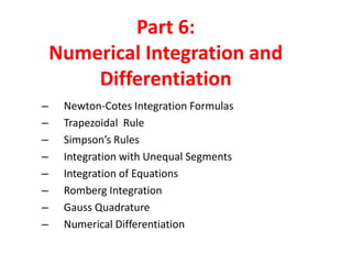
- 1. Part 6: Numerical Integration and Differentiation – – – – – – – – Newton-Cotes Integration Formulas Trapezoidal Rule Simpson’s Rules Integration with Unequal Segments Integration of Equations Romberg Integration Gauss Quadrature Numerical Differentiation
- 2. Newton-Cotes Integration Formula Replacing the complicated integrand function or tabulated data by an approximating function such as a polynomial. f(x) f(x) Replacing by a straight line x Replacing by a parabola x These formulas are applicable to both closed forms (i.e., data points at the beginning and end of the integration limits are known) and open forms (otherwise). These formulas are applied for equally spaced intervals.
- 3. Trapezoidal Rule Complicated integrand function is replaced by a first order polynomial (straight line). b I f(x) b f ( x ) dx a f 1 ( x ) dx a where the first-order polynomial f1 ( x ) f (a ) f (b ) f (a ) b b I f (a ) f (b ) (b a I (b a) a (x a) a f (a ) (x a ) dx a) f (a ) f (b ) 2 Trapezoidal rule b x
- 4. f(x) f(a)+f(b) 2 =average height f(a) I ( width ) ( average height ) f(b) b a x width All the Newton-Cotes formulas can be formulated in general form above (only definition of average height changes). Error for trapezoidal rule: b '' f ( x ) dx Et 1 '' f ( )( b 12 Local truncation error a) 3 Ea 1 12 (b 3 '' a) f '' f a (b a) Average of the second derivative between the interval
- 5. EX: Numerically integrate f ( x) 0 .2 25 x 200 x 2 675 x 3 900 x 4 400 x 5 from a=0 to b=0.8. Find the error. (Note that the exact solution is 1.6405). f (0) 0 .2 f ( 0 .8 ) Et I 0 .8 0 .2 0 . 1728 2 0 . 232 1 . 6405 0 . 232 0 . 1728 1 . 4677 t 89 . 5 % Normally, we don’t have the knowledge of the true error; we can calculate the approximate error. We need to calculate the second derivative of the function: '' f ( x) 400 4050 x 10800 x 2 8000 x 3 0 .8 400 '' f 4050 x 10800 x 0 Ea 12 8000 x 3 60 0 .8 1 2 ( 60 )( 0 . 8 ) 3 0 2 . 56 Et and Ea have the same order and sign
- 6. Multiple-application trapezoidal rule: We can increase the accuracy of the integration by dividing the interval into many segments and apply the trapezoidal rule to each segment. f(x) For n+1 equally spaced base points, there are n segments of step size: h (b a) n I h 2 x0 h n 1 f ( x0 ) 2 f ( xi ) f ( xn ) i 1 Initial point x1 final point x2 x
- 7. or n 1 f ( x0 ) I (b 2 f ( xi ) f ( xn ) i 1 a) 2n width average height Error for the multiple-application trapezoidal rule is found by summing individual errors. b Et a 12 n or 3 n '' f ( i) 3 i 1 n Ea b a 12 n 2 '' 3 '' f where f ( '' f i 1 n i ) Convergence: Error is inversely related to the square of n !
- 8. EX: Use two-segment trapezoidal rule to integrate f ( x) 0 .2 2 675 x f ( 0 .4 ) 25 x 2 . 456 200 x 3 900 x 4 400 x 5 From a=0 to b=0.8. n=2 h=0.4 f (0) I 0 .8 0 .2 0 .2 2 ( 2 . 456 ) 0 . 232 f ( 0 .8 ) 0 . 232 1 . 0688 4 Ea 1 . 6405 1 12 ( 2 ) 2 ( 60 )( 0 . 8 ) 3 t 34 . 9 % 0 . 64 Error is inversely related to the square of n. 1.0688 34.9 3 1.3695 16.5 1.4848 9.5 5 0 . 57173 I 4 1 . 0688 n 2 Et 1.5399 6.1 6 1.5703 4.3 7 1.5887 3.2 8 1.6008 2.4 t
- 9. Simpson’s Rules f(x) Instead of using a line segment, use higher-order polynomials to connect points increase the accuracy. Simpson’s 1/3 rule x1 x0 A parabola is substituted for the function. Lagrange polynomial forms are used for the replacement. Replacing Lagrange polynomials for the function at three points x0 , x1, and x2 : (x x2 I x0 x1 )( x ( x0 x2 ) x1 )( x 0 (x x 0 )( x ( x2 x 0 )( x 2 x2 ) f ( x0 ) x1 ) x1 ) f ( x2 ) (x x 0 )( x ( x1 x 0 )( x1 x2 ) x2 ) f ( x1 ) dx x2 x
- 10. After integration and algebraic manipulations 1h I 3 f ( x0 ) 4 f ( x1 ) f x2 Simpson’s 1/3 rule. In another form: I (b f ( x0 ) a) 4 f ( x1 ) f x2 h=(b-a)/2 6 width average height Error for the single segment Simpon’s 1/3 rule: Et (b a) 2880 5 f (4) > It is more accurate than expected as the error is related to the forth order derivative (third order term is meaningful but is zero). > It yields exact results for cubic polynomials even though it is obtained from a parabola.
- 11. EX: Use single application of Simpson’s 1/3 rule to integrate f ( x) 0 .2 2 675 x f ( 0 .4 ) 2 . 456 25 x 200 x 3 900 x 4 400 x 5 from a=0 to b=0.8. n=2 h=0.4 f (0) I 0 .8 0 .2 0 .2 4 ( 2 . 456 ) 0 . 232 f ( 0 .8 ) 0 . 232 1 . 3675 6 Et 1 . 6405 1 . 3675 0 . 273 t 16 . 6 % 0 .8 f (4) ( x) 21600 f 48000 x (4) f (4) 0 2400 0 .8 Ea (b a) 2880 5 (4) f ( 0 .8 ) 2880 5 ( 2400 ) ( x ) dx 0 . 273 0 Et and Ea are equal because the integrand is a fifth order polynomial
- 12. Multiple-application Simpson’s 1/3 rule For n segments: h (b a) n Total integral can be represented x2 I xn x4 f ( x ) dx x0 f ( x ) dx ... x2 f ( x ) dx xn 2 Substituting Simpson’s 1/3 formula n 1 f ( x0 ) I (b a) 4 n 2 f ( xi ) 2 i 1, 3 , 5 f ( xi ) i 2,4,6 3n width average height f ( xn )
- 13. Error for the multiple (n) segment Simpon’s 1/3 rule is calculated by adding error for individual segments. Hence, we get: Et (b a) 180 n 4 5 (4) f Multiple application Simpson’s rule returns very accurate results compare to trapezoidal rule. It is the method of choice for most applications. As for all Newton-Cotes formulas, the intervals must be equally spaced. Because of the need for three points for applications, the method is limited to odd number of points (even number of segments).
- 14. EX: Use multiple application Simpson’s 1/3 rule (n=4) to integrate f ( x) 2 675 x f ( 0 .2 ) 1 . 288 3 . 464 f ( 0 .8 ) 0 . 232 3 . 464 ) 2 ( 2 . 456 ) 0 .2 25 x 200 x 3 900 x 4 400 x 5 from a=0 to b=0.8. n=4 h=0.2 f (0) f ( 0 .6 ) I 0 .8 0 .2 4 (1 . 288 0 .2 f ( 0 .4 ) 0 . 232 2 . 456 1 . 6235 12 Et Ea 1 . 640533 1 . 623467 a) 5 180 ( n ) 4 (b (4) f 0 . 017067 ( 0 .8 ) t 1 . 04 % 5 180 ( 4 ) 4 ( 2400 ) 0 . 017067 Small error shows very accurate results are obtained.
- 15. Simpson’s 3/8 rule Simpson’s 3/8 rule is used when the odd-number of segments are encountered. A third-order polynomial is used for replacing the function. b I b f ( x ) dx f 3 ( x ) dx a a Applying a third order Legendre polynomial to four points gives I 3h f ( x0 ) 8 I (b a) 3 f ( x1 ) f ( x0 ) 3 f ( x2 ) 3 f ( x1 ) 3 f ( x2 ) 8 width f x3 average height f x3 Simpson’s 3/8 formula. h=(b-a)/3
- 16. Truncation error for Simpson’s 3/8 rule: Et (b a) 5 f (4) 6480 Simpson’s 3/8 rule is somewhat more accurate than 1/3 rule In general Simpson’s 1/3 rule is the method of choice because of obtaining third order accuracy and using three points instead of four. 3/8 rule has the utility when the number of segments is odd. In practice, use 1/3 rule for all the even number of segments and use 3/8 rule for the remaining last three segments. Higher-order Newton-Cotes formulas: Higher order (n=4,5) formulas have the same order error as n=1 (Trapezoid) or n=2,3 (Simpson’s) formulas. Higher-order formulas are rarely used in engineering practices. To increase the accuracy, just increase the number of segments!
- 17. Integration with Unequal Segments There may be cases where the spacing between data points may not be even (e.g., experimentally derived data points) One way is to use trapezoidal rule for each segment I h1 f ( x0 ) f ( x1 ) 2 h2 f ( x1 ) f ( x2 ) 2 .. hn f ( xn 1 ) f ( xn ) 2 width of the segments (h) are not constant so the formula cannot be written in a compact form. A computer algorithm can easily be developed to do the integration for unequal-sized segments. The algorithm can be constructed such that, use Simpson’s 1/3 rule wherever two consecutive equal-sized segments are encountered, and use 3/8 rule wherever three consecutive equal-sized segments are encountered. When adjacent segments are unequal-sized , just use trapezoidal rule.
- 18. Open Integration Formulas There may be cases where integration limits are beyond the f(x) range of the data. General characteristics and order of error for open forms of the NewtonCotes formulas are similar to the closed forms. Even segment formulas are usually the method of choice as they require fewer points. a b x Open forms are not used for definite integration. They have utility for analyzing improper integrals (discussed later). They have connection to multi-step method for solving ordinary differential equations.
- 19. Integration of Equations Use of multiple-application of trapezoidal and Simpson’s rules are not convenient for analyzing integration of functions. > Large number of operations required to evaluate the functions. > For large values of n, round of errors starts to dominate. Percent relative error Previously discussed methods are appropriate for tabulated data. If the function to be integrated is available, other modified methods are available. > Romberg integration (Richardson extrapolation) > Gauss quadrature Newton-Cotes method for functions: Trapezoidal rule Simpson’s rule n
- 20. Romberg Integration It uses the trapezoidal rule, but much more efficient results are obtained through iterative refinement techniques . Richardson’s extrapolation: A sequence acceleration method to improve the rate of convergence. It offers a very practical tool for numerical integration and differentiation. Application of iterative refinement techniques to improve the error at each iteration. For each iteration I exact integral I (h) E (h) approximate integral truncation error In Richardson extrapolation, two approximate integrals are used to compute a third more accurate integral.
- 21. Assume that two integrals with step sizes of h1 and h2 are available. Then, I ( h1 ) E ( h1 ) I ( h2 ) E ( h2 ) (b Error for multiple-equation trapezoidal rule ( n b E a 2 h '' h f 12 Assuming same f ’’ for two step sizes 2 1 2 2 E ( h1 ) h E ( h2 ) h 2 or E ( h1 ) E ( h2 ) h1 h2 a) )
- 22. Inserting the error to the previous equation, and solving for E(h2) E ( h2 ) I ( h1 ) 1 I ( h2 ) h1 / h 2 2 Then, I 1 I ( h2 ) ( h1 / h 2 ) 2 1 I ( h2 ) I ( h1 ) It can be shown that the error for above approximation is O(h4) although the error from use of trapezoidal rule is O(h2). For the special case of interval being halved (h2=h1/2), we get I 4 3 O(h4) I ( h2 ) 1 3 I ( h1 ) O(h2)
- 23. EX: For the numerical integration of f ( x) 0 .2 25 x 200 x 2 675 x 3 900 x 4 400 x 5 we previously obtained the following, using trapezoidal rule. n h I 1 0.8 0.1728 89.5 2 0.4 1.0688 34.9 4 0.2 1.4848 9.5 t Use Romberg integration approach to obtain improved approximations. use n=1 and n=2 for a improved approximation 4 1 I (1 . 0688 ) ( 0 . 1728 ) 1 . 367467 3 3 t 16 . 6 % If use n=2 and n=4 I 4 3 (1 . 4848 ) 1 3 (1 . 0688 ) 1 . 623467 t 1 .0 %
- 24. The method can be generalized, e.g. combine two O(h4) approximation to obtain an O(h2) approximation, and so on… Using two improved O(h4) approximations in the previous examples, we can use the following formula I 16 15 Im 1 15 Il Im: more accurate approx. Il: less accurate approx. to obtain an O(h6) approximation. Similarly, two O(h6) approximation can be combined to obtain an O(h8) approximation I 64 63 Im 1 63 Il Im: more accurate approx. Il: less accurate approx. This sequential improvement convergence technique is named under the general approach of Richardson's extrapolation.
- 25. EX: In the previous example use the two O(h4) approximations to obtain an O(h6) approximation for the integral. I 16 (1 . 623467 ) 15 1 (1 . 367467 ) 1 . 640533 15 True result is 1.640533 (correct answer to 7 S.F.!). Algorithm: O(h2) O(h4) … … … … … … … … … … Trapezoidal rule O(h6) … … … … … … … … O(h8) …
- 26. Gauss Quadrature In Newton-Cotes formulation, predetermined and evenly spaced data are used. Points of integration are covered by the data. In Gauss quadrature, points of integration are undetermined. f(x) f(x) a b x a b x For the example above, integral approximation can be improved by using two wisely chosen interior points. Gauss quadrature offer a method to find these points.
- 27. Method of undetermined coefficients: Assume two points (x0, x1) so that the integral can be written in the form I c0 f ( x0 ) f(x) f(x1) f(x0) c1 f ( x1 ) c‘s: constants -1 x0 x1 1 This requires calculation of four unknowns. We choose these four equations according to our preference. We can choose a function value that is exact to third order. x 1 c0 f ( x0 ) c1 f ( x1 ) 1dx 2 1 1 c0 f ( x0 ) c1 f ( x1 ) xdx 1 0 In general, integration limits can be made -1..1 for any integral by a simple change of variables.
- 28. 1 c0 f ( x0 ) 2 c1 f ( x1 ) x dx 2 3 1 1 c0 f ( x0 ) 3 c1 f ( x1 ) x dx 0 1 Or, by evaluating the function values c0 c1 c0 x0 2 c1 x1 c x 3 c0 x 2 0 c1 x 1 c0 x0 2 1 1 3 0 2 3 0 By these deliberate choices, we force these two points give a an integral that is exact to cubic order.
- 29. Solving for the unknowns c0 c1 1 1 x0 x1 0 . 5773503 ... 3 1 0 . 5773503 ... 3 Then, I f( 1 3 ) f( 1 3 ) Two-point GaussLegendre formula
- 30. To change (normalize) the limits of integration, we do the following change of variable: x a0 a1 x d For the lower limit (x=a a xd=-1 ) a0 a1 ( 1) For the upper limit (x=b b (b a0 2 xd=1 ) a0 a1 a1 (1) a) (b a) 2 Substitute into the original formula: x (b a) (b a ) xd 2 Differentiate both sides: dx (b a) 2 dx d These equations are subsituted into the original integrand to transfrom into suitable form for application to Gauss-Legendre formula
- 31. EX: Use two-point Gauss-Legendre quadrature formula to integrate f ( x) 0 .2 25 x 200 x 2 675 x 3 900 x 4 400 x 5 from x=0 to x=0.8 (remember that exact solution I=1.640533). First, perform a change of variable to convert the limits -1..1: x 0 .4 dx 0 .4 x d 0 . 4 dx d Substitute into the original equation to get: 0 .8 ( 0 .2 2 25 x 200 x 0 .2 25 ( 0 . 4 675 x 3 900 x 4 5 400 x ) dx 0 1 1 675 ( 0 . 4 0 .4 x d ) 0 .4 x d ) 3 200 ( 0 . 4 900 ( 0 . 4 0 .4 x d ) 0 .4 x d ) 2 4 400 ( 0 . 4 0 .4 x d ) 5 0 . 4 dx d RHS is suitable for evaluation using Gauss quadrature. Evaulating for -1/√3 (=0.516741) and for 1/√3 (=1.305837), and gives the following result: I 0 . 516741 1 . 305837 1 . 822578 t 11 . 1 % Equivalent to third order accuracy in Simpson’s method.
- 32. Higher-point formulas: Higher-point versions of Gauss quadrature can be developed in the form I c0 f ( x0 ) c1 f ( x1 ) ... n: number of points cn 1 f ( xn 1 ) For example, for 3 point Gauss-Legendre formulas, c’s and x’s are: c0 c1 c2 x0 x1 0 . 774596669 0 .0 x2 0 . 5555556 0 . 8888889 0 . 5555556 0 . 774596669 Et ~ f(6)( ) Error for Gauss Quadrature: Et 2 (2n 2n 3 (n 3) ( 2 n 1)! 4 2 )! 3 f (2n 2) ( ) n= number of points minus one 1 1
- 33. EX: Use three-point Gauss quadrature formula for the previous problem. Using the tabulated c and x values we write: I 0 . 5555556 f ( 0 . 7745967 ) 0 . 8888889 f ( 0 ) 0 . 5555556 f ( 0 . 7745967 ) which is I 0 . 2813013 0 . 8732444 0 . 4859876 1 . 640533 exact to 7 S.F.!
- 34. Numerical Differentiation Types of Differentiation: Forward expansion of Taylor series: '' f ( xi 1 ) f ( xi ) ' f ( xi ) h f ( xi 1 ) ' f ( xi ) f ( xi ) h 2 ... h=step size 2! f ( xi ) O (h) h first forward difference Backward expansion of Taylor series '' f ( xi 1 ) f ( xi ) ' f ( xi ) ' f ( xi ) h f ( xi ) f ( xi ) f ( xi 1 ) h 2 ... 2! O (h) h first backward difference Subtract forward expansion from the backward expansion: ' f ( xi ) f ( xi 1 ) 2h f ( xi 1 ) 2 O (h ) centered difference
- 35. Higher-accuracy Differentiation Formulas: High-accuracy diffentiation formulas can be obtained by adding more terms in Taylor expansion. Forward Taylor series expansion: '' f ( xi 1 ) f ( xi ) ' f ( xi ) f ( xi ) h h 2 ... 2 or ' f ( xi ) f ( xi 1 ) '' f ( xi ) f ( xi ) h h 2 O (h ) 2 Approximate the second derivative using finite difference formula '' f ( xi ) f ( xi 2 ) 2 f ( xi 1 ) h 2 f ( xi )
- 36. Then, ' f ( xi ) f ( xi 1 ) f ( xi ) f ( xi 2 ) 2 f ( xi 1 ) h 2h f ( xi ) 2 h 2 O (h ) or, f ( xi ' f ( xi ) 2 ) 4 f ( xi 1 ) 3 f ( xi ) forward scheme 2 O (h ) 2h Backward and centered finite difference formulas can be derived in a similar way: 3 f ( xi ) ' f ( xi ) ' f ( xi ) f ( xi 4 f ( xi 1 ) f ( xi 2 ) backward scheme 2 O (h ) 2h 2 ) 8 f ( xi 1 ) 12 h 8 f ( xi 1 ) f ( xi 2 ) 4 O (h ) centered scheme
- 37. EX: Calculate the approximate derivative of f ( x) 0 .1 x 4 0 . 15 x 3 0 .5 x 2 0 . 25 x 1 .2 at x=0.5 using a step size of h=0.25 (true value=-0.9125). First, evaluate the following data points: xi-2=0 ; f(xi-2)=1.2 xi+1=0.75 ; f(xi+1)=0.6363281 xi-1=0.25 ; f(xi-2)=1.103516 xi+2=1 ; f(xi+2)=0.2 xi=0.5 ; f(xi)=0.925 Forward difference scheme: 0 .2 ' f ( xi ) 4 ( 0 . 6363281 ) 3 ( 0 . 925 ) 0 . 859375 t 5 . 82 % t 3 . 77 % 2 ( 0 . 25 ) Backward difference scheme: ' f ( 0 .5 ) 3 ( 0 . 925 ) 4 (1 . 035156 ) 1 . 2 0 . 878125 2 ( 0 . 25 ) Centered difference scheme: ' f ( xi ) 0 .2 8 ( 0 . 6363281 ) 8 (1 . 035156 ) 1 . 2 12 ( 0 . 25 ) 0 . 9125 t 0%
- 38. Richardson Extrapolation: As done for the integration, Richardson extrapolation uses two derivatives of different step sizes to obtain a more accurate derivative. In a similar fashion applied for the integration, use two step sizes such that h2=h1/2. Richardson extrapolation recursive formula: D 4 3 O(h4) D ( h2 ) 1 3 D ( h1 ) O(h2) [centered difference scheme] The approach can be iteratively used by Romberg algorithm to get higher accuracies.
- 39. EX: Use Richardson extrapolation of step sizes h=0.5 and h=0.25 to calculate the derivative of the function f ( x) 0 .1 x 4 0 . 15 x 3 0 .5 x 2 0 . 25 x 1 .2 at x=0.5. Centered scheme finite difference approximation for h=0.5: 0 .2 D ( 0 .5 ) 1 .2 1 .0 t 1 9 .6 % Centered scheme finite difference approximation for h=0.25: D ( 0 .5 ) 0 . 6363281 1 . 103516 0 . 934375 t 0 .5 2 .4 % Apply Richardson extrapolation for improved accuracy: D ( 0 .5 ) 4 3 ( 0 . 934375 ) 1 3 ( 1) 0 . 9125 t 0%
- 40. Derivatives of Unequally Spaced Data In the previous discussion, both finite difference approximations and Richardson extrapolation reqires evenly distributed data. So, these methods are more suitable to evaulate functions. Emprically derived data, experimental or from field surveys, are usually not even. One way is to fit a second-order Lagrange interpolating polynomial to each set of three data points. Derivative of the polynomial: 2x ' f ( x) ( xi 1 xi x i )( x i xi 1 1 xi 1 ) f ( xi 1 ) 2x ( xi xi 1 x i 1 )( x i xi 1 xi 1 ) f ( xi ) 2x ( xi 1 xi 1 x i 1 )( x i xi 1 xi ) f ( xi 1 ) Using above formula, any point in the range of three data points can be evaluated. This equation has the same accuracy of high-accuracy centered difference approximation even though data is not need to be equally spaced.
- 41. Derivatives and Integrals for Data with Error: Differentiation process amplifies the error: y dy/dt x x As a remedy, fit a smoother function (low-order polynomial) to the uncertain data. On the other hand, integration process reduces the error. (Succusive negative and positive errors cancel out during integration). No further action is required.