1. Lecture Notes – Machine Learning Intro
CS405
Symbolic Machine Learning
To date, we’ve had to explicitly program intelligent behavior into the computer. It
would be nice if the machine could learn the intelligent behavior itself, as people learn
new material.
Herbert Simon defines learning as: “any change in a system that allows it to perform
better the second time on repetition of the same task or on another task drawn from the
same population.”
This implies:
• Generalization from experience, performance should improve not only on
repetition of the same task, but also on similar tasks
• From limited experience, generalize to unseen instances of the domain
In the following lectures we’ll study symbolic learning. These approaches process
symbols to generate new rules, usually in the context of a classifier system. A classifier
system essentially makes a prediction and some have proposed that this is a fundamental
feature of human brains – we’re always predicting something. Later we will study
connectionist approaches which can operate at a lower level than symbols. Finally, we’ll
examine genetic and evolutionary learning.
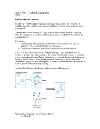
Learning algorithms may be characterized among several dimensions:
Representation language: e.g. predicate calculus:
size(X,small).

2. size(X,medium).
size(X,large).
color(Obj,Color).
shape(Obj, Style).
Concept space: Ways we can combine our representation language, e.g.:
color(X, green) ^ size(X,large)
color(X, blue) ^ size(X, large) ^ shape(X, square)
… etc …
This will generally be an exponentially large space of concepts
Goals: What we want to learn, e.g. concept of a ball
Acquired knowledge: color(X,Y) ^ size(X,Z) ^ shape(X, round)
An object any color or size but must be round
We’ll start with the problem of learning through induction. In induction, the learner is
given specific examples of the thing to be learned, and the learner must generalize the
examples into the rule. This differs from deductive reasoning, which would follow
chains of logic to reach a conclusion, much like forward chaining.
Example: Given the following Input/Output instances:
Input Output
101001 0
111001 1
001111 1
Determine the rule for producing the output (in this case it’s a multiplexer function, but it
could be symptoms for cancer patients, flower classification, etc.). We would need many
more input examples to determine the relationship.
Example with humans: Learning names of objects. Dangling food in front of baby and
learning that the thing is “food”. People may say “eat” or “pretty baby” or “coo coo!” or
even different types of food. Yet somehow children will learn the proper names of the
objects. This is an example of inductive learning in the presence of noisy input data
(noisy data=possibly incorrect or confusing data).
We can view these problems as Classification Problems. Given some evidence or input
data, determine the correct classification for the data. Some scientists argue that
intelligent human action is essentially a non-stop classification process. Next we will
examine a few methods for performing machine learning and classification.
Rote Learning
The simplest form of learning is rote learning, or simply the memorization of the input.
If the exact same input or evidence reappears, we just look into memory and spit out the

3. answer. Obviously this method leaves much to be desired, as it will fail on novel inputs
and requires large amounts of storage.
Nevertheless, rote learning is often very useful. Recall Samuel’s checkers playing
program, where rote learning allowed his system to learn how to look farther ahead in the
game tree.
Nearest Neighbor
In this method, we store all the instances we’ve seen so far as with rote learning.
However, when a new case arrives, nearest neighbor will look up the pattern in the table
of samples; if it’s there, the classification is used. If not, then the “closest” pattern or
neighbor is selected, and then the class of that pattern is used as the classification of the
new.
Example: if given below
101001 0
111001 1
001111 1
New input 001110 is similar to the last entry (using number of misplaced bits) so
the classifier would predict 001110 is 1.
The nearest neighbor classifier is a member of a family of classifiers called k-nearest
neighbor classifiers. Instead of finding the single nearest neighbor, the k-nearest
neighbors are found, where k is some constant, and the decision rule is to select the class
that appears most frequently among the k neighbors. An odd number of neighbors are
used so that ties will not occur.
Distance metric for closeness is usually: absolute distance, euclidean distance, various
normalized distance metrics
Example:
Age Sex Class
48 1 1
60 0 1
25 1 2
38 0 2
Given a new record, age=55, sex=1 (male) then using the absolute distance metric, the
new case will be assigned to class 1 because the distance to the second case, with a value
of |60-55|+|1-0| = 6 is the smallest.
Note that age dominates the distance metric since it has the largest range of values. This
is often undesirable, so a common operation is to normalize all of the input features so

4. they have a value between 0 and 1. To do this we simply find the range for that feature
and divide each value by the range after subtracting the min:
Age:
48
60
25
38
Range: 25 to 60 (range of 60 – 25 = 35)
48 becomes (48 – 25) / 35 = 0.657
60 becomes (60 – 25) / 35 = 1
25 becomes (25 – 25) / 35 = 0
38 becomes (38 – 25) / 35 = 0.0857
Our new data set becomes:
Age Sex Class
0.657 1 1
1 0 1
0 1 2
0.0857 0 2
Given a new record, age=55, sex=1 (male) this is mapped to: age = (55 – 25) / 35 =
0.857 and sex = 1. The distance to the first case becomes |0.857-0.657| + |1-1| = 0.2 and
the distance to the second case now becomes |0.857 – 1| + |1-0| = 1.14 so now we would
pick the first case over the second case (although we’d still predict the class to be 1).
This approach is often used with “social information filtering” or “recommendation
engines” in which records become user ratings for various items and the nearest neighbor
is found for rated items.
For example, consider a movie service like Netflix. Say there are users U1 to U5 and
there are movies M1 to M9. Users rate movies from 1 (bad) to 5 (good). The ratings
could be stored in a table like so:

5. M1 M2 M3 M4 M5 M6 M7 M8 M9
U1 3 2 5 5 4
U2 1 4 5 4 3 4 5
U3 2 1 4 4 2 3 2
U4 3 2 2 2 5 2 5 2
U5 1 4 5 5 4
Now, a new user, U6, comes along, and rates:
M2 = 1
M3 = 4
M4 = 4
If we perform a nearest neighbor search then we can find other moviegoer(s) with similar
tastes. In this case, U2 is almost an exact match for the three movies for U6. It is only
off by 1 for M4. The recommendation engine might then recommend M9 because U2
seems to make similar ratings to U6, but U6 hasn’t rated M9 yet.
Netflix had a contest where they make a subset of their customer data available and
invite users to write their own movie recommendation algorithms. From their website,
http://www.netflixprize.com :
To qualify for the $1,000,000 Grand Prize, the accuracy of your submitted
predictions on the qualifying set must be at least 10% better than the accuracy
Cinematch can achieve on the same training data set at the start of the Contest.
To qualify for a year’s $50,000 Progress Prize the accuracy of any of your
submitted predictions that year must be less than or equal to the accuracy value
established by the judges the preceding year.
In 2007 a team from BellCore won the grand prize!
Amazon takes a similar approach recommending items you might want to buy.

6. Nice features of nearest neighbor classification:
Easy to implement
Often very effective
Some variability with selecting number of neighbors
Bad points:
Need to store all cases, can take a lot of space
May be hard to come up with good distance metric
Noisy data is sometimes a problem
Statistical Inference
The next classifier we’ll look at is the Bayesian classifier. First, we should cover some
statistical concepts and look at statistical inference.
Independent Events – two events A and B are independent if and only if the probability
of their both occurring is equal to the product of their occurring individually. In other
words, the two events have no relation to one another. The independence relation is
expressed:
p(A ∩ B) = p(A) * p(B)
This reads, the probability of events A and B together is identical to the probability of A
multiplied by the probability of B.
For example, consider rolling two six sided dice. The probability that die 1 = 1 and die 2
= 6 would be:
p(Die1=1 ∩ Die2=6) = p(Die1=1) * p(Die2=6)
Out of the 36 possible dice roll combinations, there is only one where die1=1 and
die2=6. Therefore, p(Die1=1 ∩ Die2=6) = 1/36.
p(Die1=1) is 1/6 and p(Die2=6) is 1/6 so we end up with 1/36 = (1/6) * (1/6) = 1/36
so the independence relation is satisfied.
There are many events that are not independent. For example, consider the case where A
is your name = Barack Obama, and B is you are the POTUS.
p(name=Barack Obama ∩ you=POTUS) = p(name=Barack Obama) * p(you=POTUS) ?
p(you=POTUS) is 1/pop-USA, and p(name=Barack Obama) = (num BO’s/pop-USA).
However, p(name=Barack Obama ∩ you=POTUS) is much higher because there is a
dependency between people named Barack Obama and presidents of the United States.
This probability is 1/num BO’s, which is much higher than the right hand side of the
relation.

7. Here is an example of probabilistic inference. Suppose you have statistics about traffic
in Anchorage based on observations of traffic locations.
S is a Boolean random variable that is t or f to indicate if traffic slowed down
A indicates if there was an accident when S was observed
C indicates if there was road construction when S was observed
We might have a table of probabilities for these variables:
S C A p
T T T 0.01
T T F 0.03
T F T 0.16
T F F 0.12
F T T 0.01
F T F 0.05
F F T 0.01
F F F 0.61
For example, this indicates that the probability of traffic slowing when there was an
accident but no construction is the third row of 0.16.
From these outcomes we can calculate the probability of simple or complex events. For
example, we can calculate the probability of a traffic slowdown S. It is the sum of the
first four lines: 0.01+0.03+0.16+0.12 = 0.32.
We could also calculate the probability of construction with no slowdown, this would be
expressed as p(C ∩ !S) and would be the sum of the 5th and 6th lines, or 0.01 + 0.05 =
0.06.
A Venn diagram representation is a good way to visualize the probabilities.
The collection of this statistical data can be a useful form of machine learning. For
example, once collected, if we ever encounter construction and an accident then we are
looking at p=0.01 for C,A and S, and p=0.01 for C, A, and !S. This means we can
predict a 50% chance of a slowdown.
Conditional Probability

8. So far we’ve been looking at the Prior Probability. This is the probability of an event
prior to any new evidence and is symbolized by p(event).
Another kind of probability is Posterial Probability. This is a form of conditional
probability which is the probability of an event given some new evidence. The posterior
probability is symbolized by p(event | evidence) and reads “the probability of the event
given the evidence”.
Consider a person having disease d, from a set of diseases D, with symptom or evidence
s, from a set of symptoms S. Then:
p(d|s) = | d ∩ s| / |s|
The right hand side is the number of people having both the disease d and the symptom s
divided by the total number of people having the symptom s:
Since the sample space for determining the probabilities of the numerator and
denominator are the same, we get:
p(d|s) = p(d ∩ s) / p(s) (1)
There is an equivalent relationship for p(s|d):
p(s|d) = p(s ∩ d) / p(d)
Solving for p(s ∩ d) yields: p(s ∩ d) = p(s|d) * p(d) (2)
We can substitute (2) into (1) to yield:
p(d|s) = p(s|d) * p(d) / p(s)
This says that the posterior probability of the disease given the symptom is the likelihood
of the symptom given the disease, normalized by the probability of the symptom.
Bayesian Classifiers
These classifiers are statistically based using Bayes Theorem, which is derived from the
previous equation of conditional probability. If a particular instance of evidence appears
with more than one class, the best prediction, i.e. the prediction with the minimum error

9. rate, is to choose the class that occurs most frequently. For example, if the evidence = X
and the class=0 occurs 1000 times while the evidence = X and the class=1 occurs 10
times, then 0 is the class that should be predicted when evidence X occurs.
Bayesian induction follows directly from the Bayes rule. The goal is to find the
probability of a class C, given evidence e:
P(e| C)P(C)
P(C| e) =
P(e)
Note that evidence e may consist of many observations. For example, in the traffic
example, e might be that there was an accident but no construction. In this situation, C
would correspond to whether or not there was a slowdown.
Consider the case where there are three classes. Then we have:
P(e | C1 )P(C1 )
P(C1 | e) =
P(e)
P(e | C 2 )P(C 2 )
P(C 2 | e) =
P(e)
P(e | C 3 )P(C 3 )
P(C 3 | e) =
P(e)
If all we care about is to pick the most likely class, then we can ignore P(e) since it is a
common denominator. Consequently, we would pick the class that maximizes:
P(e|Ci)P(Ci)
Computing P(e|C) is the hard part; however, we can estimate it. With the assumption of
conditional independence, i.e. each piece of evidence is independent of every other piece
of evidence, then the equation can be transformed into a simple product where we
multiply all of the atomic pieces of evidence that make up e. (Recall that this assumption
is often NOT true! But it simplifies matters greatly).
When given a new object to classify, under conditional independence we simply choose
the class that maximizes the following expression derived from the Bayes Rule:
n
P(C)∏ P(e i | C)
i =1
Given a set of training data, a table of probabilities can be easily constructed to
approximate P(e|C). For example, if we are given an object with two possible
classifications (Framitz or Fuzul) determined by the single feature of color (Mauve,
Fuschia, or Azure), perhaps we collect the following observations. These observations
form the training data for the classifier:

10. Class Colors
Object 1 Framitz fuschia, mauve
Object 2 Framitz fuschia, mauve, azure
Object 3 Framitz fuschia
Object 4 Framitz fuschia
Object 5 Framitz fushcia, mauve, azure
Object 6 Fuzul fuschia, mauve, azure
Object 7 Fuzul mauve, azure
Object 8 Fuzul fuschia, azure
Object 9 Fuzul mauve, azure
Object 10 Fuzul mauve, azure
Then a table with the following probabilities could be constructed based upon the
training data:
Probability Class-Framitz Class-Fuzul
P(Class) 5/5 = 0.5 5/5 = 0.5
P(Mauve|Class) 3/5 = 0.6 4/5 = 0.8
P(Fuschia|Class) 5/5 = 1.0 2/5 = 0.4
P(Azure|Class) 1/5 = 0.2 5/5 = 1.0
In the case of the table shown above, if given a new object with colors fuschia and azure,
the probability that the object belongs in the Framitz class is (0.5)(1.0)(0.2), while the
probability that the object belongs in the Fuzul class is (0.5)(0.4)(1.0). Since the Fuzul
probability is higher, the Fuzul class is predicted.
Note that we can constantly update the probabilities in the table to reflect new data as it
comes in; consequently the system is learning as the table gets updated.
If we don’t assume conditional independence, one thing we can try is assuming singular
dependence; i.e. consider the probability of two pieces of evidence together. This greatly
increases the size of the table necessary to store the probability values.
Nice features of Bayesian Classifiers:
Easy to implement, can give good results
Do not need to store every case, only counters and probabilities
Can deal with noisy data
Bad points:
Harder to implement w/o conditional independence assumption
Linear Discriminants
The conditional independence assumption with Bayes Rule is actually a form of a linear
discriminant. Essentially we are trying to separate classes by a single line:

11. Class1 Class2
Here, we are attempting to separate instances in space by a single line, where one side of
the line denotes one class, and the other side denotes a different class. Many problems
are not completely separable in this fashion, such as the XOR function:
Class=1
1 0
Class=0
0 1
In this example, the best a linear classifier can do is 75%. It is impossible to draw a
single line in the XOR space where all cases of class 0 are on one side and all cases of
class 1 are on the other. We can still solve these problems with linear classifiers, if we
introduce non-linearities somewhere in the process; e.g. when picking the features. The
other alternative is to combine the features in a non-linear fashion (not a linear
classifier). Later we will briefly look at Support Vector Machines (SVM’s). A support
vector machine uses a kernel to map inputs to a higher dimensional space using a non-
linear function and then attempts to find linear vectors that separate the classes.
Testing Classifier Systems
How do we test to see if our classifier system is any good? The typical method is to
separate our data set into two sets: a training set, and a test set. The training set is used to
design the classifier, and the test set is used strictly for testing. If we “hide” the test cases
and only look at them after the classifier is complete, then we have a way to determine
the error on the new cases.
The error rate can be defined as: error rate = number of errors / number of cases

12. The error rate on the test cases is the test sample error.
Both sets of data should be selected randomly from the population. How many test cases
do we need so that the test sample error approaches the true error rate? Not very many!
A typical split to use is 2/3 training and 1/3 testing.
The approach described so far is for a single train-and-test experiment. If we were
unlucky and didn’t pick good random samples, we might have skewed results. A better
method is to perform multiple train-and-test experiments. This is called random
subsampling.
The best random subsampling technique is “leave one out”. In leave one out, given n
samples a classifier is generated using n-1 cases and tested on the single remaining case.
This is repeated n times, each time leaving a different case out. The error is then the
number of total errors on the single test cases divided by n.
This technique has been proven to be superior to other error techniques, but it is very
expensive to run for large data sets. In this case, a common technique is to use cross-
validation.
In k-fold cross-validation, the cases are split up into k approximately equal-sized groups.
For each group, training is performed on all of the other groups and testing is performed
on that one group. The average error rates over all the k partitions is the cross-validated
error rate. A typical number used is 10-fold cross validation.
Error Definitions
It is often useful to distinguish between the different types of errors that are made. To do
this, we can construct a confusion matrix. A confusion matrix for a binary classification
is shown below:
Class Positive Class Negative
Prediction + # True Positive # False Positive
Prediction - # False Negative # True Negative
Given this table, we can now compute various other metrics:
Accuracy = (TP + TN) / (TN + TP + FN + FP)
Precision = TP / TP + FP
Recall = TP / TP + FN
Neg Precision = TN / TF + FN
Neg Recall = TN / TN + FP
We’ll revisit these concepts when we talk about information retrieval.