1. MACHINE LEARNING SOLUTIONS FOR
TRANSPORTATION NETWORKS
by
as ˇ
Tom´ˇ Singliar
MS, University of Pittsburgh, 2005
Submitted to the Graduate Faculty of
Arts and Sciences in partial fulfillment
of the requirements for the degree of
Doctor of Philosophy
University of Pittsburgh
2008

2. UNIVERSITY OF PITTSBURGH
ARTS AND SCIENCES
This dissertation was presented
by
as ˇ
Tom´ˇ Singliar
It was defended on
Nov 13, 2008
and approved by
Miloˇ Hauskrecht, Computer Science, University of Pittsburgh
s
Rebecca Hwa, Computer Science, University of Pittsburgh
Gregory F. Cooper, DBMI and Computer Science, University of Pittsburgh
Geoffrey J. Gordon, Machine Learning Department, Carnegie Mellon University
G. Elisabeta Marai, Computer Science Department, University of Pittsburgh
Dissertation Director: Miloˇ Hauskrecht, Computer Science, University of Pittsburgh
s
ii

3. MACHINE LEARNING SOLUTIONS FOR TRANSPORTATION NETWORKS
as ˇ
Tom´ˇ Singliar, PhD
University of Pittsburgh, 2008
This thesis brings a collection of novel models and methods that result from a new look at practical problems
in transportation through the prism of newly available sensor data. There are four main contributions:
First, we design a generative probabilistic graphical model to describe multivariate continuous densities
such as observed traffic patterns. The model implements a multivariate normal distribution with covariance
constrained in a natural way, using a number of parameters that is only linear (as opposed to quadratic) in
the dimensionality of the data. This means that learning these models requires less data. The primary use
for such a model is to support inferences, for instance, of data missing due to sensor malfunctions.
Second, we build a model of traffic flow inspired by macroscopic flow models. Unlike traditional such
models, our model deals with uncertainty of measurement and unobservability of certain important quantities
and incorporates on-the-fly observations more easily. Because the model does not admit efficient exact
inference, we develop a particle filter. The model delivers better medium- and long- term predictions than
general-purpose time series models. Moreover, having a predictive distribution of traffic state enables the
application of powerful decision-making machinery to the traffic domain.
Third, two new optimization algorithms for the common task of vehicle routing are designed, using the
traffic flow model as their probabilistic underpinning. Their benefits include suitability to highly volatile
environments and the fact that optimization criteria other than the classical minimal expected time are
easily incorporated.
Finally, we present a new method for detecting accidents and other adverse events. Data collected from
highways enables us to bring supervised learning approaches to incident detection. We show that a support
vector machine learner can outperform manually calibrated solutions. A major hurdle to performance of
supervised learners is the quality of data which contains systematic biases varying from site to site. We build
a dynamic Bayesian network framework that learns and rectifies these biases, leading to improved supervised
detector performance with little need for manually tagged data. The realignment method applies generally
to virtually all forms of labeled sequential data.
iii

4. TABLE OF CONTENTS
PREFACE . . . . . . . . . . . . . . . . . . . . . . . . . . . . . . . . . . . . . . . . . . . . . . . . . . . x
1.0 INTRODUCTION . . . . . . . . . . . . . . . . . . . . . . . . . . . . . . . . . . . . . . . . . . 1
1.1 Pieces of the puzzle . . . . . . . . . . . . . . . . . . . . . . . . . . . . . . . . . . . . . . . . . 2
2.0 TRAFFIC FLOW DATA . . . . . . . . . . . . . . . . . . . . . . . . . . . . . . . . . . . . . . 4
2.1 Traffic flow data collection . . . . . . . . . . . . . . . . . . . . . . . . . . . . . . . . . . . . . 4
2.2 Traffic patterns . . . . . . . . . . . . . . . . . . . . . . . . . . . . . . . . . . . . . . . . . . . 5
3.0 A STATIC DESCRIPTION OF TRAFFIC PATTERNS . . . . . . . . . . . . . . . . . . 8
3.1 Introduction . . . . . . . . . . . . . . . . . . . . . . . . . . . . . . . . . . . . . . . . . . . . . 8
3.2 State of the art . . . . . . . . . . . . . . . . . . . . . . . . . . . . . . . . . . . . . . . . . . . 9
3.2.1 Joint probability (generative) models . . . . . . . . . . . . . . . . . . . . . . . . . . . 9
3.2.1.1 Modeling conditional independence . . . . . . . . . . . . . . . . . . . . . . . 10
3.2.1.2 Dimensionality reduction and latent space models . . . . . . . . . . . . . . . 11
3.2.1.3 Mixture models . . . . . . . . . . . . . . . . . . . . . . . . . . . . . . . . . . 12
3.2.1.4 Nonparametric models . . . . . . . . . . . . . . . . . . . . . . . . . . . . . . 12
3.2.2 Conditional (discriminative) models . . . . . . . . . . . . . . . . . . . . . . . . . . . . 13
3.3 Gaussian Tree Models . . . . . . . . . . . . . . . . . . . . . . . . . . . . . . . . . . . . . . . 13
3.3.1 Mixture of Gaussian Trees . . . . . . . . . . . . . . . . . . . . . . . . . . . . . . . . . 14
3.3.2 Inference in the MGT Model . . . . . . . . . . . . . . . . . . . . . . . . . . . . . . . . 15
3.3.3 Learning in the MGT Model . . . . . . . . . . . . . . . . . . . . . . . . . . . . . . . . 15
3.4 Experimental Evaluation . . . . . . . . . . . . . . . . . . . . . . . . . . . . . . . . . . . . . . 17
3.4.1 Data . . . . . . . . . . . . . . . . . . . . . . . . . . . . . . . . . . . . . . . . . . . . . 17
3.4.2 Evaluation metrics . . . . . . . . . . . . . . . . . . . . . . . . . . . . . . . . . . . . . 18
3.4.3 Evaluation setup and parameters . . . . . . . . . . . . . . . . . . . . . . . . . . . . . 19
3.4.4 Evaluation results . . . . . . . . . . . . . . . . . . . . . . . . . . . . . . . . . . . . . . 20
3.5 Conclusions . . . . . . . . . . . . . . . . . . . . . . . . . . . . . . . . . . . . . . . . . . . . . 22
4.0 PROBABILISTIC TRAFFIC PREDICTION WITH A DYNAMIC MODEL . . . . . 24
4.1 Introduction . . . . . . . . . . . . . . . . . . . . . . . . . . . . . . . . . . . . . . . . . . . . . 24
iv

5. 4.2 State of the art . . . . . . . . . . . . . . . . . . . . . . . . . . . . . . . . . . . . . . . . . . . 25
4.2.1 Microscopic models . . . . . . . . . . . . . . . . . . . . . . . . . . . . . . . . . . . . . 25
4.2.2 Macroscopic models . . . . . . . . . . . . . . . . . . . . . . . . . . . . . . . . . . . . . 26
4.2.2.1 Demand characterization . . . . . . . . . . . . . . . . . . . . . . . . . . . . . 26
4.2.2.2 Fundamental diagrams . . . . . . . . . . . . . . . . . . . . . . . . . . . . . . 28
4.2.3 Learning approaches . . . . . . . . . . . . . . . . . . . . . . . . . . . . . . . . . . . . 29
4.2.3.1 Time-series models . . . . . . . . . . . . . . . . . . . . . . . . . . . . . . . . . 29
4.2.3.2 Kalman filters . . . . . . . . . . . . . . . . . . . . . . . . . . . . . . . . . . . 30
4.2.3.3 Other learning paradigms . . . . . . . . . . . . . . . . . . . . . . . . . . . . . 31
4.2.4 Hybrid models . . . . . . . . . . . . . . . . . . . . . . . . . . . . . . . . . . . . . . . . 31
4.3 The dynamic flow model . . . . . . . . . . . . . . . . . . . . . . . . . . . . . . . . . . . . . . 31
4.3.1 Flow conservation dynamics . . . . . . . . . . . . . . . . . . . . . . . . . . . . . . . . 32
4.3.2 Volume-speed characteristic . . . . . . . . . . . . . . . . . . . . . . . . . . . . . . . . 33
4.3.3 Fundamental diagram representations . . . . . . . . . . . . . . . . . . . . . . . . . . . 35
4.3.4 Intersections and interchanges . . . . . . . . . . . . . . . . . . . . . . . . . . . . . . . 36
4.3.5 Inference . . . . . . . . . . . . . . . . . . . . . . . . . . . . . . . . . . . . . . . . . . . 38
4.4 Experimental evaluation . . . . . . . . . . . . . . . . . . . . . . . . . . . . . . . . . . . . . . 40
4.4.1 Data . . . . . . . . . . . . . . . . . . . . . . . . . . . . . . . . . . . . . . . . . . . . . 40
4.4.2 Experimental setup and baselines . . . . . . . . . . . . . . . . . . . . . . . . . . . . . 40
4.4.3 Evaluation metrics . . . . . . . . . . . . . . . . . . . . . . . . . . . . . . . . . . . . . 41
4.4.4 Experimental results . . . . . . . . . . . . . . . . . . . . . . . . . . . . . . . . . . . . 41
4.5 Conclusions . . . . . . . . . . . . . . . . . . . . . . . . . . . . . . . . . . . . . . . . . . . . . 42
5.0 ROUTING PROBLEMS IN TRAFFIC NETWORKS . . . . . . . . . . . . . . . . . . . . 47
5.1 Introduction . . . . . . . . . . . . . . . . . . . . . . . . . . . . . . . . . . . . . . . . . . . . . 47
5.2 State of the art . . . . . . . . . . . . . . . . . . . . . . . . . . . . . . . . . . . . . . . . . . . 49
5.2.1 Shortest path . . . . . . . . . . . . . . . . . . . . . . . . . . . . . . . . . . . . . . . . 49
5.2.2 Markov Decision processes . . . . . . . . . . . . . . . . . . . . . . . . . . . . . . . . . 50
5.2.3 Stochastic shortest path . . . . . . . . . . . . . . . . . . . . . . . . . . . . . . . . . . 51
5.2.4 Semi-Markov models . . . . . . . . . . . . . . . . . . . . . . . . . . . . . . . . . . . . 51
5.2.5 Other approaches to non-stationary cost distributions . . . . . . . . . . . . . . . . . . 51
5.2.6 Practical and complexity issues . . . . . . . . . . . . . . . . . . . . . . . . . . . . . . 52
5.2.7 Continuous state space . . . . . . . . . . . . . . . . . . . . . . . . . . . . . . . . . . . 53
5.3 The traffic route navigation problem . . . . . . . . . . . . . . . . . . . . . . . . . . . . . . . 53
5.3.1 SMDP formulation of the navigation problem . . . . . . . . . . . . . . . . . . . . . . 54
5.4 SampleSearch network planning algorithm . . . . . . . . . . . . . . . . . . . . . . . . . . . . 56
5.4.1 Approximate Bellman updates . . . . . . . . . . . . . . . . . . . . . . . . . . . . . . . 56
v

6. 5.4.2 Time-dependent A∗ pruning . . . . . . . . . . . . . . . . . . . . . . . . . . . . . . . . 57
5.4.3 Algorithm description . . . . . . . . . . . . . . . . . . . . . . . . . . . . . . . . . . . . 57
5.4.4 Online search . . . . . . . . . . . . . . . . . . . . . . . . . . . . . . . . . . . . . . . . 58
5.5 The k-robust algorithm . . . . . . . . . . . . . . . . . . . . . . . . . . . . . . . . . . . . . . . 60
5.5.1 An online version of k-robust . . . . . . . . . . . . . . . . . . . . . . . . . . . . . . . . 62
5.6 Experimental comparison . . . . . . . . . . . . . . . . . . . . . . . . . . . . . . . . . . . . . 63
5.6.1 Experimental setup . . . . . . . . . . . . . . . . . . . . . . . . . . . . . . . . . . . . . 63
5.6.2 Evaluation metric . . . . . . . . . . . . . . . . . . . . . . . . . . . . . . . . . . . . . . 64
5.6.3 Baseline heuristics . . . . . . . . . . . . . . . . . . . . . . . . . . . . . . . . . . . . . . 64
5.6.4 Experimental results . . . . . . . . . . . . . . . . . . . . . . . . . . . . . . . . . . . . 64
5.6.5 Volatility experiment . . . . . . . . . . . . . . . . . . . . . . . . . . . . . . . . . . . . 68
5.6.5.1 Link failure model . . . . . . . . . . . . . . . . . . . . . . . . . . . . . . . . . 68
5.6.5.2 Evaluation setup . . . . . . . . . . . . . . . . . . . . . . . . . . . . . . . . . . 68
5.6.5.3 Evaluation results . . . . . . . . . . . . . . . . . . . . . . . . . . . . . . . . . 68
5.7 Conclusions . . . . . . . . . . . . . . . . . . . . . . . . . . . . . . . . . . . . . . . . . . . . . 70
6.0 LEARNING TO DETECT INCIDENTS . . . . . . . . . . . . . . . . . . . . . . . . . . . . 72
6.1 Introduction . . . . . . . . . . . . . . . . . . . . . . . . . . . . . . . . . . . . . . . . . . . . . 72
6.2 State of the art . . . . . . . . . . . . . . . . . . . . . . . . . . . . . . . . . . . . . . . . . . . 73
6.3 Supervised learning for incident detection . . . . . . . . . . . . . . . . . . . . . . . . . . . . 74
6.3.1 Traffic incident data . . . . . . . . . . . . . . . . . . . . . . . . . . . . . . . . . . . . . 75
6.3.2 Performance metrics . . . . . . . . . . . . . . . . . . . . . . . . . . . . . . . . . . . . . 75
6.3.3 The California 2 model . . . . . . . . . . . . . . . . . . . . . . . . . . . . . . . . . . . 76
6.3.4 Evaluation framework . . . . . . . . . . . . . . . . . . . . . . . . . . . . . . . . . . . . 77
6.3.5 Feature selection . . . . . . . . . . . . . . . . . . . . . . . . . . . . . . . . . . . . . . . 78
6.3.6 Dynamic Naive Bayes . . . . . . . . . . . . . . . . . . . . . . . . . . . . . . . . . . . . 81
6.3.7 The SVM detector . . . . . . . . . . . . . . . . . . . . . . . . . . . . . . . . . . . . . . 82
6.3.7.1 Persistence checks . . . . . . . . . . . . . . . . . . . . . . . . . . . . . . . . . 83
6.4 Overcoming noise and bias in labels . . . . . . . . . . . . . . . . . . . . . . . . . . . . . . . . 83
6.4.1 A model for label realignment . . . . . . . . . . . . . . . . . . . . . . . . . . . . . . . 85
6.4.2 Inference for realignment . . . . . . . . . . . . . . . . . . . . . . . . . . . . . . . . . . 86
6.4.3 Learning and transfer to new locations . . . . . . . . . . . . . . . . . . . . . . . . . . 86
6.5 Evaluation . . . . . . . . . . . . . . . . . . . . . . . . . . . . . . . . . . . . . . . . . . . . . . 87
6.5.1 Data . . . . . . . . . . . . . . . . . . . . . . . . . . . . . . . . . . . . . . . . . . . . . 87
6.5.2 Experimental setup and model parameters . . . . . . . . . . . . . . . . . . . . . . . . 88
6.5.2.1 Naive Bayes slices . . . . . . . . . . . . . . . . . . . . . . . . . . . . . . . . . 88
6.5.2.2 TAN slices . . . . . . . . . . . . . . . . . . . . . . . . . . . . . . . . . . . . . 88
vi

7. 6.5.3 Evaluation results . . . . . . . . . . . . . . . . . . . . . . . . . . . . . . . . . . . . . . 91
6.6 Conclusions . . . . . . . . . . . . . . . . . . . . . . . . . . . . . . . . . . . . . . . . . . . . . 91
7.0 CONCLUSION AND FUTURE CHALLENGES . . . . . . . . . . . . . . . . . . . . . . . 93
7.1 Contributions . . . . . . . . . . . . . . . . . . . . . . . . . . . . . . . . . . . . . . . . . . . . 93
7.2 Open problems . . . . . . . . . . . . . . . . . . . . . . . . . . . . . . . . . . . . . . . . . . . 94
7.2.1 Partial observability . . . . . . . . . . . . . . . . . . . . . . . . . . . . . . . . . . . . . 94
7.2.2 New data . . . . . . . . . . . . . . . . . . . . . . . . . . . . . . . . . . . . . . . . . . . 94
7.2.3 Temporal noise in sensing and inference . . . . . . . . . . . . . . . . . . . . . . . . . . 95
7.2.4 Spatial vector fields . . . . . . . . . . . . . . . . . . . . . . . . . . . . . . . . . . . . . 95
7.2.5 From single vehicle to multi-vehicle route optimization . . . . . . . . . . . . . . . . . 95
APPENDIX. GLOSSARY . . . . . . . . . . . . . . . . . . . . . . . . . . . . . . . . . . . . . . . . 97
BIBLIOGRAPHY . . . . . . . . . . . . . . . . . . . . . . . . . . . . . . . . . . . . . . . . . . . . . . 99
vii

8. LIST OF TABLES
1 Results for mixture-of-trees experiments . . . . . . . . . . . . . . . . . . . . . . . . . . . . . . 21
2 Comparison of fundamental diagram representations . . . . . . . . . . . . . . . . . . . . . . . 36
3 Volume RMS error results for ARMA . . . . . . . . . . . . . . . . . . . . . . . . . . . . . . . 44
4 Volume RMS error results for dynamic model . . . . . . . . . . . . . . . . . . . . . . . . . . . 44
5 Likelihood error results for ARMA . . . . . . . . . . . . . . . . . . . . . . . . . . . . . . . . . 45
6 Volume RMS error results for dynamic model . . . . . . . . . . . . . . . . . . . . . . . . . . . 45
7 Off-line planning results, first setup . . . . . . . . . . . . . . . . . . . . . . . . . . . . . . . . . 65
8 Online planning results, first setup . . . . . . . . . . . . . . . . . . . . . . . . . . . . . . . . . 66
9 Off-line planning results, second setup . . . . . . . . . . . . . . . . . . . . . . . . . . . . . . . 67
10 Results of the synthetic volatility experiment . . . . . . . . . . . . . . . . . . . . . . . . . . . 69
11 The “anchoring” conditional probability table for DBN model of incidents . . . . . . . . . . . 82
12 Evaluation sites for incident detection . . . . . . . . . . . . . . . . . . . . . . . . . . . . . . . 89
13 Incident detection performance results . . . . . . . . . . . . . . . . . . . . . . . . . . . . . . . 91
viii

9. LIST OF FIGURES
1 The road network in Pittsburgh with placement of sensors. . . . . . . . . . . . . . . . . . . . 5
2 Daily traffic profiles . . . . . . . . . . . . . . . . . . . . . . . . . . . . . . . . . . . . . . . . . 6
3 Local flow properties . . . . . . . . . . . . . . . . . . . . . . . . . . . . . . . . . . . . . . . . . 6
4 Significance plots for mixture-of-trees experiments . . . . . . . . . . . . . . . . . . . . . . . . 23
5 MetaNet model overview . . . . . . . . . . . . . . . . . . . . . . . . . . . . . . . . . . . . . . 27
6 Fundamental diagram representations . . . . . . . . . . . . . . . . . . . . . . . . . . . . . . . 28
7 Traffic quantities mapped to a highway schematic . . . . . . . . . . . . . . . . . . . . . . . . . 32
8 Segmentation and intersection schematic . . . . . . . . . . . . . . . . . . . . . . . . . . . . . . 34
9 Non-parametric fundamental diagram conditioning . . . . . . . . . . . . . . . . . . . . . . . . 34
10 Smoothing, filtering and prediction . . . . . . . . . . . . . . . . . . . . . . . . . . . . . . . . . 38
11 Bayesian network interpretation of the dynamic model . . . . . . . . . . . . . . . . . . . . . . 39
12 Dynamic model posteriors . . . . . . . . . . . . . . . . . . . . . . . . . . . . . . . . . . . . . . 46
13 The sample-based tree roll-out of an MDP. . . . . . . . . . . . . . . . . . . . . . . . . . . . . 59
14 The block scheme of the k-robust planning algorithm . . . . . . . . . . . . . . . . . . . . . . . 62
15 Incident effect illustration . . . . . . . . . . . . . . . . . . . . . . . . . . . . . . . . . . . . . . 75
16 A section of traffic data annotated with incidents . . . . . . . . . . . . . . . . . . . . . . . . . 76
17 AMOC curves for basic variate detectors . . . . . . . . . . . . . . . . . . . . . . . . . . . . . . 78
18 AMOC curves of temporal derivative detectors . . . . . . . . . . . . . . . . . . . . . . . . . . 79
19 AMOC curves of spatial derivative detectors . . . . . . . . . . . . . . . . . . . . . . . . . . . . 80
20 AMOC curves for simple learning detectors . . . . . . . . . . . . . . . . . . . . . . . . . . . . 80
21 Structure and performance of dynamic naive Bayes detector . . . . . . . . . . . . . . . . . . . 81
22 Performance changes with persistence check setting . . . . . . . . . . . . . . . . . . . . . . . . 83
23 Performance of the SVM detector for different feature sets . . . . . . . . . . . . . . . . . . . . 84
24 The realignment graphical model structure . . . . . . . . . . . . . . . . . . . . . . . . . . . . 85
25 Convergence of accident position labeling . . . . . . . . . . . . . . . . . . . . . . . . . . . . . 88
26 Effect of data quality on SVM detector performance . . . . . . . . . . . . . . . . . . . . . . . 89
ix

10. PREFACE
There are many people without whom this thesis would never see the light of day. The biggest thanks go,
in equal share, to my advisor Professor Miloˇ Hauskrecht and my wife, Zuzana Jurigov´. Miloˇ has been
s a s
my guide through the world of research, teaching me the art of science. It is to him that I owe my first real
touches with the field of artificial intelligence and machine learning, which I suspect will remain my lifelong
fascination. It boggles my mind to imagine the efforts he had to expend to provide me with all the funding,
time and resources that it took to get it done. He celebrated with me in good times and stood behind me
in tough ones. I can only hope he will remain a mentor and a friend for a long time. Thank you!
Zuzana has been by my side through it all and she must never leave. She is wisdom in my foolishness,
safe arms in my fear, a gentle push when I cannot go on alone. She is more to me that can be put in words.
Just - thank you!
I am very grateful to all mentors who helped me along, inspired, advised and admonished me. My special
thanks belongs to the members of my thesis committee who gave generously from their time and expertise
to help chisel this capstone: Professors Greg Cooper, Geoff Gordon, Rebecca Hwa and Liz Marai. The AI
faculty at the department have always been there to critique ideas, broaden horizons and spark new thoughts.
Professors Rebecca Hwa, Diane Litman and Jan Wiebe taught me about processing natural language, maybe
the ultimate feat in artificial intelligence. Many of the other faculty at the Department of Computer Science
also left a lasting impression in me. When I grow up, I’d like to have Bob Daley’s sharp wit with which he
approaches both life and research, Kirk Pruhs’ depth of knowledge and teach like John Ramirez. Thanks!
Dr. Daniel Mosse has led many projects that sustained my research with funding.
I am thankful for the inspiration that is Dr. Roger Day, someone in whom exceptional qualities as a
teacher, researcher and above all, a kind and compassionate human being are combined. Professors Louise
Comfort and J S Lin were collaborators who each brought a different perspective into my thinking about
infrastructure and complex systems and made me appreciate the vastness of the world behind these academic
walls.
It was a great thing for me to meet Dr. Denver Dash, who led me through the aspects of doing great
research outside of academia and who is always a wellspring of the craziest innovative ideas. The work with
him also allowed me to meet Dr. Eve Schooler and many of the admirable people at Intel.
Thank you all!
x

11. Parts of this thesis and closely related work were published at
• ECML-2007 [147], the European Conference on Machine Learning,
• PKDD-07 [146], the Conference on Principles and Practice of Knowledge Discovery in Data,
• ICML-06 Workshop on Machine Learning in Event Detection [145],
• ISAIM-08 [148], the International Symposium on AI and Math and
• UAI-08 [143], the Conference on Uncertainty in Artificial Intelligence.
This thesis is dedicated to my wife Zuzana who has always supported me unflinchingly; and our parents,
who gave up our presence for us to pursue goals distant in space and time.
as ˇ
Tom´ˇ Singliar
xi

12. 1.0 INTRODUCTION
Transportation networks are among the most complex artifacts developed by humans. Accurate models of
such systems are critical for understanding their behavior. Traffic systems have been studied with the help
of physics-inspired traffic models and traffic simulators. The model parameters would be tweaked until the
predictions of the model agreed with empirically collected evidence. However, the evidence was often scarce
and hard to collect. As a result, the models were often less than robust.
A fundamental shift has occurred with advances in sensor instrumentation and automatic traffic data
collection. Traffic sensors today are capable of measuring a variety of traffic-related quantities, such as speed
and vehicle counts. Data collected from the many sensors now placed on highways and roads provides a novel
opportunity to better understand the behavior of complex systems, including local and global interactions
among traffic flows in different parts of a transportation network.
The main objective of this work is to study methods and tools that make use of the traffic sensor data
to build better and more robust traffic models and use them to support a variety of inference, decision
making and monitoring tasks. A unifying theme is the application of machine learning and statistical
modeling methodology. The work straddles the boundary between theory and application. In the process
of attacking transportation management issues, novel models and algorithms are contributed to machine
learning: the mixture-of-Gaussian-trees generative model, the sequence label realignment framework with
its associated general inference algorithm, and new planning algorithms that can robustly handle highly
uncertain environments.
Numerous decision-making protocols in road traffic management are outdated in the sense that they do
not realize the full potential of the recently increased availability of traffic flow data. Solutions for common
tasks are based on algorithmic problems formulated with simple inputs, commensurate with limited data-
collection capabilities in the past. As the explosive developments in information collection capabilities
that we experienced in the last few decades transformed the data foundation of decision making, many
established algorithmic problem formulations have suddenly become oversimplifications of the actual problem
of optimizing with respect to all available information.
Management of traffic with the goal of maximizing throughput is important to areas with increasing
demand and congestion. Consequently, much hope rests with Intelligent Transportation Systems (ITS) as a
solution that will enable a greater density of transportation. ITS put a variety of new sensing and actuation
1

13. equipment at the fingertips of civil engineers and computer scientists: an unprecedented extent of sensor
and camera networks, integration with cell phone networks and onboard GPS. Control capabilities such as
1
ramp metering, reversible lane control and variable signal timing have been around for some time, but
new efficiencies are now made possible by the data revolution. The need to use the actuation capabilities
effectively opens new classes of optimization problems.
The central challenge standing before us is the scale and complexity of behavior of the underlying physical
system. Traffic flow is the result of many seemingly-random human decisions combined together through
natural and social laws. It is subject to feedback effects such as grid locking and phase transitions such as
jam formation. Machine learning algorithms often surprise us with their ability to disentangle, or at least
imitate such complex dependencies; and we show here that they can also be fruitfully applied to this domain.
For instance, I develop a stochastic model of traffic flow that uses sensor and infrastructure information
to characterize and predict behavior of vehicular traffic in time and space. The main purpose of such models
is operate within the context of an Intelligent Transportation System to support decision tasks faced by
those who are responsible for the functioning of transportation networks, as well as by those who consume
their services. Current traffic flow models operate with deterministic quantities and are calibrated by expert
judgment. A statistical modeling approach leveraging sensor data enables this redesign along the lines of
stochasticity and automated calibration from data.
Our work on vehicular traffic models generalizes to other complex network systems that underpin our
lifestyle: transportation, distribution and communication infrastructure.
1.1 PIECES OF THE PUZZLE
The research is divided into four main chapters: Chapter 3 develops a generative model to describe traffic
patterns generated by the highway system. In Chapter 4, I design a macroscopic dynamic probabilistic model
for road traffic prediction. Chapter 5 explores optimization problems of vehicle routing using the dynamic
model. Chapter 6 describes a sequential data realignment framework to aid in supervised learning of traffic
incident detection.
Naturally, the aims of the respective chapters interlock: The path search and optimization algorithms of
the Chapter 5 require an estimate of the future costs of traversing road segments. These are provided by
predictive inference in the Markov model of traffic flow state built in Chapter 4. While this is the main use
of the flow model in the dissertation, it is a general flow model with wider uses, examples of which include
anomaly detection and modeling the effects of disturbances such as construction. The models developed
in Chapter 3 have the basic goal of supporting other efforts with clean data and a description of traffic
behavior. A density-estimation approach is taken at the macroscopic level (entire network), where a model
1 The Glossary on page 97 defines these and other traffic management terms used throughout the thesis.
2

14. of the flow volume distribution is learned and used to fill in missing values. Chapter 6 capitalizes on the
gained insights and makes a step towards automatically calibrated incident detection models by casting the
problem as supervised learning. The biggest hurdle there appears in a (perhaps) surprising place: the biased
and noisy labeling of the incident data. I develop a dynamic Bayesian network formulation to rectify the
bias. In yet another example of practical problems inspiring theoretical developments, it turns out that the
exponentially faster inference algorithm used for the “cleaning” network generalizes to a class of dynamic
Bayesian networks that often appear in diagnostic and detection tasks.
But first things first: let us have a look at the data.
3

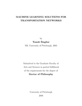
15. 2.0 TRAFFIC FLOW DATA
Summary. In this chapter we describe the traffic data that we have available and which will serve to train
and evaluate our models. It is intended to give a degree of familiarity with the data and basic traffic patterns.
2.1 TRAFFIC FLOW DATA COLLECTION
The data are collected by a network of sensors, mostly loop detectors1 operated in the Pittsburgh metropoli-
tan area by a private company under contract from Pennsylvania Department of Transportation (PennDOT).
There are about 150 active sensors that record data about the traffic flow at their respective locations. To
get a sense of their placement, please refer to Figure 1.
Typically, each mainline lane has a separate loop detector and data is reported per lane. It is rare for
off-ramps and onramps to have a detector. Whenever one lane has a sensor, all mainline lanes going in the
same direction do. The collection of lane sensors in the same location is referred to as a detector station.
These stations report various quantities regularly to the Traffic Management Center, using a data network
built alongside the highways. Three traffic quantities are normally observed and aggregated over a time
period: the average speed, volume (number of passing vehicles) and occupancy (the percentage of road
length taken up by cars—“traffic density”). The aggregation of our data is at 5-minute intervals; the
observed shorter-interval volumes are summed, the occupancies and speeds are averaged.
Two years worth of data are available to us, the entire years 2003 and 2004. On average, about 12% of
the data are missing. However, they do not miss uniformly at random as missing data are often a result of
a single detector failure that normally takes several days to be repaired. Quality tends to be better in the
central region of the city. Data quality information is included in the form of a counter that says how many
basic detector cycles yielded a measurement that is valid from the standpoint of the internal quality control
algorithm of the sensor. Most of the time, the counter stands at its maximum value.
The data has been imported to a MySQL database and indexed to support the various queries we will
need.
1 See the Glossary (page 97) for definitions of traffic management terms. In the electronic version of this thesis, traffic
management terms are made into clickable links to the Glossary.
4

16. 29
Sensors
51
18
50
44
27
2598
17
48
2658
2638
16 268 2563
267
43
2576
2560 633
613
2615
2599
49
2657
2
9637 254
6
2656
2
8636
2655
2635
26
5 47
393
2
1
269 374
271 417
416
56459
415
414
2596
270 2557
255 2695
673
653 1631
293259
294 34 36 2575 2597
32
11 1633 1634
2595 373 258
273
2676
2675
10 260 274
262
275
30
272
264
266
52
280 265
−80.08 −80.06 −80.04 −80.02 −80 −79.98 −79.96 −79.94 −79.92 −79.9
Figure 1: The road network in Pittsburgh with placement of sensors.
2.2 TRAFFIC PATTERNS
Global. The overarching traffic pattern is the diurnal variation and the workday/weekend dichotomy.
Workday traffic volumes exhibit a characteristic variation with high volumes during the rush hours and
lower volumes at other times. Furthermore, some sensors mainly register traffic in the morning hours
(inbound sensors), some have their peaks in afternoon hours (outbound sensors) and many have a mixed
traffic pattern. A typical volume profile is shown in Figure 2. Slight but consistent differences are also
observed between workdays.
Local. Let us look at the saturation effects that arise when the number of vehicles entering a road
segment grows beyond a certain limit. The throughput of a roadway increases linearly with the number of
cars entering it until the point of a phase transition when the traffic starts to jam and throughput declines.
This is demonstrated by Figure 3a: The correlation of volume and speed is positive at lower volumes, but
negative at high volumes that occur during the daily peaks.
It is a part of traffic manager’s expert knowledge that to keep the traffic flowing freely, you need about
one lane for each 1200 cars per hour in order to prevent traffic from backing up. Figure 3b, looking at one
sensor, confirms that this seems to be the case. The sensor has 4 lanes, so 400 cars in 5 minutes corresponds
to 1200 cars per hour per lane. The horizontal (x-) axis represents speed, while the y-axis represents the
5

17. Sensor 47, direction inbound Sensor 47, direction outbound
1200 1200
1000 1000
800 800
600 600
400 400
200 200
0 0
0 1 2 3 4 5 6 7 8 9 10 11 12 13 14 15 16 17 18 19 20 21 22 23 24 0 1 2 3 4 5 6 7 8 9 10 11 12 13 14 15 16 17 18 19 20 21 22 23 24
(a) Inbound sensor flow profile (b) Outbound sensor flow profile
Figure 2: Daily traffic profiles. Time is on the horizontal axis, hourly volumes per lane on the vertical one.
Both profiles represent sensor 47, a) in the inbound direction, b) in the outbound direction.
600
Daily profile: Correlation between speed and volume, total volumes
0.6 450
volume (# of vehicles)
400
0.4
500
350
0.2
400
300
Number of cars
0
250
300
speed−volume
200
−0.2 correlation
150 200
−0.4
100
−0.6 100
50
−0.8 0
0 50 100 150 200 250 300
Time after midnight (x5 minutes) 0
0 10 20 30 40 50 60 70
Average speed in 5 min intervals
(a) Correlation of flow and speed in time (b) Joint distribution of volume and speed
Figure 3: Local flow properties. a) Volume (right y-axis) and its correlation to speed (left y-axis) during
the day (x-axis in multiplies of 5-minutes. The graph represents 24 hours.
b) Volume-speed scatterplot diagram, Ft Pitt tunnel sensor inbound. The horizontal (red in color printouts)
line represents 1200 vehicles per lane per hour.
6

18. number of cars passing. Each point is therefore a paired measurement of car count and speed. Most of the
time, the traffic is uncongested and vehicles pass at a mean speed of about 50-55 miles per hour. However, at
around 300 vehicles per interval, instances of lowered speed begin to appear and above 400 cars per interval
(red horizontal line), the average speed decreases significantly due to congestion.
7

19. 3.0 A STATIC DESCRIPTION OF TRAFFIC PATTERNS
Summary. Traffic flow data, as any real-world measurement, suffers from missing or incorrect data and
noise. A powerful approach to these problems is to model the joint density of the data and use inference to
clean it. Our goal is to devise a model that can capture the dependencies of data dimensions that result from
interactions between traffic flows. As with all statistical models, one needs to balance the tension between
model complexity and accuracy of representation. In this chapter, a generative model called “mixture of
Gaussian trees” (MGT) is developed. It can model densities with fairly complex covariances nearly as well as
a full-covariance Gaussian, but does so with only a linear number of parameters. This squares well with the
intuition that traffic flow dependencies are local and in nature, being moderated by the physical connectivity
of the road network. We use MGT to model the joint distribution of all traffic volumes, but avoid making
any assumptions restricting its use to the particular domain.
3.1 INTRODUCTION
Density estimation is a task central to machine learning. Once a joint probability density of multiple variables
is found, it can be used to answer almost any questions about the data. No learning is, however, possible
without selecting a bias that embodies our basic assumptions about the data. Ideally, we look for a model
that is simple, can explain data well and admits efficient inference and learning algorithms. Some of these
goals are naturally opposed, for instance model complexity and accuracy.
Because so many quantities describing real-world systems are continuous-valued, continuous multivariate Contri-
bution
density estimation is an important and well studied topic and many models of varying uses have been
developed. In this chapter, a new model is proposed that stands out on low complexity, while it models the
types of continuous distributions arising in networks nearly as well as the complex (in terms of model space
dimension) multivariate Gaussian.
Traffic quantities measured at different locations on highways are not independent. Spatially close loca-
tions experience correlations due to physical interaction between their respective traffic flows. On one hand,
this makes the analysis of the network system more challenging. On the other hand, the dependencies can
be profitably used to infer information about portions of the roadway where the sensor is malfunctioning or
8

20. not present at all. To take advantage of the dependencies, models that compactly capture the covariance of
traffic variables are needed. It should also embed a model bias that matches the local nature of dependencies
in traffic networks.
We approach the problem by modeling the dependencies with the most complex1 Bayesian network
still tractable, a tree. Since different dependencies may be more prominent in different traffic modes (for
instance, times of day), we combine several trees in a mixture model. The mixture variable “selects” which
tree dependency structure best represents the particular data point.
3.2 STATE OF THE ART
Two approaches to traffic modeling exist that parallel the division that exists in machine learning: generative
joint probability models and discriminative, conditional models. The goal of a joint probability model is to
fully describe the distribution of variables in the complete high-dimensional space. Generative models are
better equipped to deal with missing values and support general probabilistic queries. Conditional models
represent conditional dependencies among (subsets of) variables. They typically do not define a full joint
probabilistic model as they lack a prior over data. Their advantage is that they usually directly optimize
the desired performance metric.
3.2.1 Joint probability (generative) models
The multivariate Gaussian [47] is the most commonly used distribution, as it naturally arises in very many Multi-
variate
problems. It also appears to be well suited for modeling traffic volumes [12]. The number of cars passing Gaussian
during a given interval can be thought of as a result of a stochastic process in which drivers choose to take the
particular segment with a fixed probability p, resulting in a binomial distribution of the number of observed
cars. The binomial distribution, for large N , is well approximated by the Gaussian. The multivariate
Gaussian model is characterized by its mean µ and covariance matrix Σ. It is described by the probability
density function (pdf)
1
p(x; µ, Σ) = exp x − µ)Σ−1 (x − µ)
(2π)d |Σ|
The covariance matrix Σ is assumed to be positive semi-definite. The parameters are usually learned from
observed traffic data using maximum-likelihood estimates. The quality of the estimate depends on the
number N of data points available. One learning disadvantage of the Gaussian distribution is that the
number of its parameters grows quadratically in the number of dimensions, leading to high uncertainty of
the covariance estimate. The problem of parameter dimensionality can be addressed by introduction of
independence assumptions or transformation of the original covariate space into a lower-dimensional one.
1 Of course, the scale of model complexity is close to a continuum and what can be considered “tractable” depends on
application and size the problems presented.
9

21. The axis-aligned covariance Gaussian [47] assumes all variables are independent. Thus, the model ex-
plicitly disregards correlations between the component variables by restricting the covariance matrix to the
diagonal. An even more severe restriction is a spherical Gaussian with Σ = σ 2 I. The terms “axis-aligned”
and “spherical” refer to the shape and orientation of equiprobability surfaces of the probability density
function.
3.2.1.1 Modeling conditional independence Graphical models [72, 91] reduce the complexity of Bayesian
belief
the model by explicitly representing conditional independences among the variables. In general, the models networks
require smaller numbers of parameters. A Bayesian network consists of a directed acyclic graph and a
probability specification. In the directed graph, each node corresponds to a random variable, while edges
define the decomposition of the represented joint probability distribution. The probability specification is
the set of conditional distributions p(Xi |pa(Xi )), i = 1, . . . , D:
D
p(X) = p(Xi |pa(Xi )),
i=1
where pa(Xi ) are the parents of Xi in the graph. The set {Xi } ∪ pa(Xi ) is referred to as the family of Xi .
Intuitively (but not exactly), an edge in a Bayesian network represents a causal influence of the parent on
the child.2
Bayesian belief networks have been used to model both local dependencies between traffic flows at Bayes nets
and traffic
neighboring locations and global congestion patterns. In Sun et al.’s work [159, 158], the dependence structure
is constructed manually as a Bayesian network, following the road connectivity. The learning component
then reduces to parameter learning.
The JamBayes system [69] is interesting in that it learns directly to predict the occurrence of traffic jams
in Seattle area. Thus the prediction task is binary. Moreover, they attempt to predict surprising traffic jams
– those that are not easily implied by observing the time series. JamBayes uses structure learning to get a
Bayesian network suitable for their task. However, their task is very different from what we attempt here.
The space they are modeling is essentially the discrete set {0, 1}d and their data is situated within the road
network only implicitly. Learning in JamBayes optimizes prediction accuracy and the resulting structure
has very little to do with the original network.
Bayesian belief networks cannot represent cyclic interactions and dependencies well [23]. Bidirectional Markov
random
and circular interactions are better modeled by Markov random fields (MRFs) [23, 86], synonymous with fields
undirected graphical probability models [91]. MRFs model local interactions between variables by means of
local potentials ϕ. The joint distribution is given as a product of F factors:
F
1
p(x) = ϕi (x),
Z i=1
2 The exact concept of (in-)dependence in Bayesian networks is closely tied to the graph theoretical concept of directed
separation [91].
10

22. where the normalizing factor Z is such that we obtain a proper probability distribution, i.e. Z = x i ϕi (x).
Domains of the factors are cliques of the underlying graph. Ideally, a factor should range over a small sub-
set of X. In the special case of Bayesian networks, the factors correspond to the conditional probability
distributions over families.
Note that (1) the marginal of a multivariate Gaussian is a Gaussian and (2) product of two Gaussians
is a Gaussian up to a normalization constant. Hence, if the potential functions ϕi are themselves Gaussian,
the entire joint distribution implied by an MRF is a Gaussian. Gaussian MRFs do not add representative
power over a normal distribution, but may encode a multivariate normal more compactly. They are popular
in fields such as image reconstruction [54] because elegant algorithms can be formulated on pixel grids and
other regular lattices. However, they are rarely seen applied to large irregular structures where the graph
cannot be triangulated [72] neatly in advance.
Inference in general graphical models is very difficult. Even approximate inference in Bayesian networks Trees –
efficient
is NP-hard [36]. In general Markov random fields, additional difficulty lies in estimating Z, also known as inference
3
the partition function. However, tree-structured graphical models admit efficient (linear) inference, a fact
that is directly connected to their low treewidth and the complexity of the join tree algorithm [72]. This
favorable property will take a central role in the development of our algorithm.
3.2.1.2 Dimensionality reduction and latent space models Another road to reducing model com-
plexity (number of parameters) is to reduce data dimensionality. Transformations such as PCA (Principal
Component Analysis) [47] and its variants can reduce the high-dimensional multivariate space to a more com-
pact approximate representation. With PCA, the data X is projected onto a lower-dimensional subspace
such that maximum variance is retained. The original data can be reconstructed from the lower-dimensional
representation Y by means of the basis matrix V :
Xn×d ≈ Yn×k Vk×d ,
where d k. Once the data is represented with a lower dimension, any model can be used with less risk of
overfitting. In communication networks, PCA has been successfully applied [98] to decompose the network
flow data into a smaller number of component “eigenflows”. Recently [71] proposed a distributed imple-
mentation of PCA that permits an approximate computation in very high dimensional spaces by splitting
the matrix into manageable chunks, one per computation node, and bounding the error incurred by deciding
to not communicate updates between nodes.
Latent space models [16] achieve dimensionality reduction by assuming that the observed data is a noisy Latent
space
function of a lower-dimensional set of unobserved random variables. They correctly capture the real-world models
fact that behavior correlations are often caused by some common factors (time of day, weather, large events,
etc.). Latent variable models are available and being developed for a variety of data types, including the
3 Inference in GMRF is simplified by their joint normality.
11

23. classical Gaussian [162], multinomial [68, 17] and binary [138, 144]. Non-linear manifolds in the data space
can also be modeled [34].
Kalman filter is a dynamic latent space model usually thought of as a temporal tool. We will discuss Kalman
filter
them in more detail in the following chapter, focusing on state prediction. Kalman filtering can also be
applied spatially, to fill in data using the readings from neighboring sensors [56]. However, it is susceptible
to breaking at discontinuities in the flow effected by onramps, exits or change in road infrastructure [58, 59].
3.2.1.3 Mixture models The Gaussian distribution is unimodal. Mixture models [47] overcome the Mixture
models
problem of unimodality by assuming that the observations come from several different distributions. There
is an unobservable choice variable that selects which component distribution the particular data point comes
4
from. The type of the latent variable distinguishes between a mixture model (discrete) and a latent space
model (continuous). In principle, given enough components, a Gaussian mixture model can approximate any
distribution with arbitrary precision [110]. The joint probability distribution implied by a mixture model
with K components is a sum of the component distributions Mi weighted by the mixture probabilities
p(m = i):
K
p(x) = p(m = i)Mi (x), (3.1)
i=1
where m is the mixture variable and Mi is the i-th mixture component, a probability distribution over the
space of x.
3.2.1.4 Nonparametric models Non-parametric density estimation models [47, 65] eschew choosing a
particular model for the data D. Instead, the data density is estimated by putting a small kernel around
each data point xi ∈ D. If the kernel is itself a probability distribution (integrates to 1), the density implied
by the model is
|D|
1
p(x|D) = K(x, xi ), (3.2)
|D| i=1
where K(x, xi ) is the kernel function with a maximum at xi . This functional form implies high values of
p(x|D) in regions of high concentration of training data points, which is what we need. In essence, such model
can be understood as a mixture model with as many components as there are data points. The largest issue
with non-parametric model is the choice of the kernel. A popular choice for the kernel is a radial basis kernel
(such as a spherical Gaussian). We will use axis-aligned Gaussian kernels to model local traffic behavior
later. An important choice is the bandwidth of the kernels, which controls the smoothness of the resulting
distribution. For instance, a very low-variance Gaussian kernel will produce a spiky distribution with many
local maxima; increasing the variance will result in a smoother probability surface.
4 The choice variable often becomes the class variable in classification problems, leading to classification models such as LDA
(Linear) and QDA (Quadratic Discriminant Analysis) [47].
12

24. 3.2.2 Conditional (discriminative) models
Given the strong correlations between flows at points in time and space, it is not surprising to find that traffic
data imputation literature is dominated by variants of linear regression [65]. Linear regression is a mainstay
of statistical modeling. The variable of interest y is modeled as a linear combination of other covariates x:
y = θ0 + θ · x,
where θ is a vector of weights.
Chen [24] uses a spatial linear regression approach to predict volumes. The volume reading of sensor
is regressed on the readings of neighboring sensors at the same time. The paper reports a relative error of
approximately 11% with this method.
The conditional autoregressive (CAR) model embodies similar intuitions about locality as the MGT
model presented below. It was first used to model neighboring pixels in a raster image [15]. The model
assumes that the volume y(s) observed at location s is a linear combination of volumes at adjacent locations:
s
y(s) = s + θr y(r), (3.3)
r∈N (s)
s
where N (s) denotes the neighborhood of s, a parameter θr is the linear coefficient of r’s volume in s’s
2
equation, and s ∼ N (0, σs ) is Gaussian additive noise.
The intuition is that traffic flows at places not directly adjacent are unlikely to influence each other except
via the situation on a road segment(s) connecting them. In other words, a “spatial” Markov property [99]
holds. The neighborhood N (s) serves the function of the Markov blanket; that is, given the state in the
neighborhood, s is independent of the state at other locations.
[57] use a pairwise regression model with readings from neighboring lanes as input covariates together
with upstream and downstream sensor measurements. Pairwise regression is unique in that the output
variable is regressed on each input variable separately. The prediction is taken to be the median of the
predictions with the isolated covariates.
In [83], the authors consider a hypothetical ad hoc wireless network between vehicles and use an adjusted
linear-regression model to fill in the data lost due to connectivity problems inherent in such a mobile setup.
Unfortunately, the technique was not evaluated on real data and the evaluation leaves a more quantitative
methodology to be desired.
3.3 GAUSSIAN TREE MODELS
The model-complexity problem of the full multivariate Gaussian model is often avoided by assuming that all
variables are independent. As a result, the learning problem decomposes to D univariate learning problems,
13

25. where D is the dimensionality of the data. The drawback is that ignoring all interactions is unrealistic for
traffic networks that exhibit strong correlation between readings of neighboring sensors.
Our model exploits the intuitive observation that traffic variates do not causally (co-)depend if they are
associated with distant locations. The dependencies are the result of and transmitted by interactions of
physical traffic flows. Since we want to preserve the general applicability of the model, we will not restrict
the structural learning to (any derivative of) the network topology.
3.3.1 Mixture of Gaussian Trees
Bayesian networks [72] are a popular formalism for capturing probabilistic dependencies. Being based on
directed acyclic graphs, they model causal relations well. However, some application domains exhibit cyclic
causal patterns that cannot be naturally expressed as a Bayesian network, with the causes being parent
variables of the effects. For instance, traffic congestions are subject to grid locking. Undirected graphical
models such as Markov random fields avoid this representational issue, but often at a great computational
cost.
One way to address the problem of cyclic interactions is to approximate the underlying distribution with
a simpler dependence structure that permits both efficient learning and inference. Having the maximum
number of edges without introducing cycles, tree structures are a natural choice. By committing to a single
tree, we capture the maximum number of dependencies without introducing a cycle; but inevitably, some
dependencies will be ignored. In the mixture of trees model [112], the missed dependencies may be accounted
for by the remaining mixture components. Mixtures of trees are a special case of Bayesian multinets [53].
Meil˘ developed the model in a discrete variable setting [112]. The mixture of Gaussian trees (MGT)
a
model uses Gaussian instead of discrete variables. The MGT model is related to mixtures of Bayesian
networks [161], but differs in how it performs structure search. For trees, the optimal structure can be
computed exactly from mutual information, while [161] relies on a heuristic to score the candidate structures
and greedily ascend in the model space.
Let there be a set of variables X, such as measurements from different sensors in the traffic networks.
Mixture of Gaussian trees models dependencies between the random variables in X by constructing several
tree structures on the same set of variables, each tree encoding a different subset of the dependencies. The
tree structures are then combined together in a mixture model.
Definition 1 The MGT model consists of:
• a collection of m trees with identical vertex sets T1 = (X, E1 ), . . . , Tm = (X, Em ), where each node xv ∈ X
with parent xu has a conditional probability function
xv ∼ N (µv + cv xu , σv ).
Thus, a child node’s value is a noisy linear function of its parent’s value. The parameters of the conditional
probability distribution associated with the node xv are (µv , cv , σv ).
14

26. m
• mixture weights λ = (λ1 , . . . , λm ) such that λi = 1. Graphically, this can be represented by an
k=1
unobservable m-valued multinomial mixture variable z that selects which tree is “switched on”.
Because of the conditional linear Gaussian local CPDs, a distribution represented by a single tree is
jointly Gaussian, but clearly not all Gaussian distributions are representable by trees. Thus, the space of
MGT distributions is a proper subset of distributions representable by a mixture of Gaussians with the same
number m of components.5 Note that it is always possible to orient a tree so that each node has at most one
parent. Such a tree-structured directed graph encodes the same set of independencies under d-separation as
an undirected tree does under graph separation.
Let Tk (x) also denote the probability of x under the distribution implied by the tree Bayesian network
Tk . The joint probability for the mixture model is then:
m
p(x) = λk Tk (x). (3.4)
k=1
(Compare Equation 3.1.)
3.3.2 Inference in the MGT Model
Any probabilistic query in the form p(y|e) can be answered from the joint distribution (Equation 3.4) by
taking:
p(y, e) i λi Ti (y, e)
p(y|e) = = (3.5)
p(e) i λi Ti (e)
Both the numerator and denominator represent m instances of inference in tree Gaussian networks, which
is a linear-complexity problem [140] and well supported in the Bayes Net Toolbox [118] for Matlab.
3.3.3 Learning in the MGT Model
The maximum likelihood parameters for the MGT model can be obtained by the EM algorithm.
Let γk (n) denote the posterior mixture proportion:
λk Tk (xn )
γk (n) = n
.
i λi Ti (x )
The γk (n)s can be interpreted as “responsibility” of tree k for the n-th data point. Computing γk (n)s
N
constitutes the E-step. The quantity Γk = n=1 γk (n) takes on the meaning of the expected count of data
points that Tk is responsible for generating. Let us also define the distribution Pk associated with Tk over
γk (n)
the set of data points by Pk (xn ) = Γk . This distribution represents a weighting of the dataset from which
we’ll learn the structure and parameterization of Tk .
Three quantities must be estimated in each M-step: (1) the structure of trees that constitute the mixture
components, (2) their parameterization and (3) the mixture proportions.
We need to select the structure that maximizes the Gaussian likelihood of the weighted data ascribed to Tree
structure
5 which in turn is, asymptotically as m → ∞, all continuous distributions with support RD [67].
15

27. the component in the E-step. Chow and Liu [30] have shown how to accomplish this. Given any distribution
D, the Chow-Liu (CL) procedure finds an undirected graph structure that optimally approximates the
given distribution. In our case, the distribution D is given empirically as a training data set (histogram)
D = {xn , wn }N , where wn = Pk (xn ). The algorithm selects a tree model T such that the KL-divergence (or
n=1
equivalently, the cross-entropy) between the responsibilities computed in the E-step and the tree distribution
is minimized:
N
new
Tk = argmax Pk (xi ) log Tk (xi ). (3.6)
Tk i=1
Equivalently, this maximizes the marginal likelihood of the model. The minimization of the cross-entropy
is accomplished by finding a Maximum Weight Spanning Tree (MWST), where the edges are weighted by
the mutual information between variables they connect. The structure update for a tree Tk thus requires
that we compute the mutual information between all variables xu , xv ∈ X. Mutual information between xu
and xv under distribution p is defined in the discrete case as
p(xu , xv )
Ik (xu , xv ) = p(xu , xv ) log . (3.7)
xu ,xv
p(xu )p(xv )
That is, the sum is performed over all values of xu and xv , yielding O(r2 ) complexity for this step if both
xu and xv can take on r values.
In the continuous case, this is computationally infeasible without making a distributional assumption.
Since the modeling assumption is that xu and xv are jointly distributed as a mixture-of-Gaussians and
one tree is to represent one of the mixture components, we treat Pk (xi ) as a weighted sample from a
Gaussian. Estimating the parameters of the Gaussian entails computing the maximum-likelihood estimate
ˆ
of the covariance matrix Σk , from the data D weighted by the posterior contributions γk (n). Then we can
obtain the posterior mutual information for the k−th tree in closed form:
1 ˆ 2 2
Ik (xu , xv ) = − log(|Σk |/(σu σv )), (3.8)
2
ˆ 2 2
where Σk is the maximum likelihood estimate of the 2 × 2 covariance matrix of xu , xv . σu and σv are
ˆ
the diagonal elements of Σk and | · | denotes the determinant of a matrix. Intuitively, if the off-diagonal
covariance elements are large compared to the variances themselves, then knowing xv tells us much about
the value of xu . This is the meaning of mutual information.
When we have the mutual information, we can run the MWST procedure. After we have determined the
optimal structure, we orient the tree by picking a vertex at random and directing all the edges away from
it. In this manner we achieve that every vertex has at most one parent. Mutual information is symmetrical,
which means that any orientation of edges yields a spanning tree that is optimal in the Chow-Liu sense.
Once the structure is learned, we proceed to parameter learning. It is unsurprising to derive that the Parameter
learning
Γk
M-step update for λ is to match the expected empirical marginal: λk = N .
Now consider an arc u → v and recall that xv ∼ N (µv + cv xu , σv ). We have data in the form Duv =
(i) (i)
{(xu , xv , w(i) )}N ,
i=1 where the weight w(i) corresponds to Pk (xi ) computed in the E-step. We can update
16

28. the parameters of v, denoted θv = {µv , cv , σv }, by maximizing the likelihood of the data P (Duv |θv ). This is
accomplished in the standard manner of equating the derivatives of the completed log-likelihood w.r.t. cv ,
µv and σ 2 to 0. We obtain that the update of µv and cv is the solution of the following linear system:
   
N
(i)
N
(i) (i)   N
(i) (i)
 w xu w  µ
ˆ  xv w 
 n=1 i=1  v  =  i=1 . (3.9)
 N N   N 
(i) (i)
xu w
(i) (i) (i)
xu xu w cv
ˆ (i) (i) (i)
xv xu w
i=1 i=1 i=1
2
Knowing µv and cv we can estimate σv :
N −1 N
2 (i)
σv = w (x(i) − µv − cv x(i) )2 wv
v u
(i)
(3.10)
n=1 i=1
This completes the M-step description. E- and M- steps are alternated until the expected complete log-
likelihood stabilizes.
The parameter that remains to be chosen is the number of mixture components (trees). We propose that Model
selection
the search be performed by learning the model with increasing number of components until the Bayesian
Information Criterion (BIC) no longer decreases. The BIC is defined as an approximation to the integrated
likelihood [139, 29]:
ˆ
BIC(k) = −2 ln p(D|k, θk ) + ψk ln N (3.11)
ˆ
where D is the training data, θk is the ML estimate of parameters and ψk is the number of free parameters
in model with k components. BIC trades off model fit for model complexity. Note that the first term grows
approximately linearly with the number of training data points N , while the second grows logarithmically.
Thus on small datasets BIC will favor simple models, while large training sets will support more complex
models.
3.4 EXPERIMENTAL EVALUATION
While the proposed MGT model is generally applicable to any continuous multivariate distribution, its
development was inspired by traffic networks and we therefore test it on a dataset of traffic variables. The
testing task is to impute, or “fill in”, missing data. We use three metrics to compare the performance of the
MGT model to full- and diagonal-covariance Gaussians and the conditional auto-regressive model.
3.4.1 Data
The data was collected by 75 sensors monitoring the freeways in the densely connected and instrumented
central area of Pittsburgh. Each data point is thus a vector consisting of the numbers of vehicles passing
the respective sensors during a five-minute interval. The dataset contains all measurements during the time
interval between 8am and 9am of all workdays throughout one year. The correlations between sensors are
17

29. high and we expect that this will be a challenging dataset for the structure search algorithms, causing them
to capture spurious correlations.
Data from some sensors are missing, typically in either short periods (malfunctions that can be resolved
by resetting the sensor) or longer streaks (malfunctions that require servicing the sensor). Sensor outages
at distinct sensor stations appear independent, as intuitively expected. Data points with missing data were
discarded so that we have a complete dataset with observed ground truth for the evaluation. The data is
divided into training and testing sets in 70/30 random splits.
3.4.2 Evaluation metrics
In order to assess the quality of distribution modeling, we use the following metrics: a log-likelihood score,
relative error and coefficient of determination. The complexity of the model is accounted for by also reporting
the BIC score obtained in training of the model. After the model is trained on the training set, some variables
in each data point of the testing set are chosen to be hidden; they will be denoted by h(n) , while the remaining
(observed) variables will be denoted by e(n) . Denote the set of hidden variables by H.
We compute the log-likelihood score
N
LLS(H|θM ) = log p(h(n) |e(n) , θM ) (3.12)
n=1
This score reflects how well the model predicts the set of chosen values, given the remaining observations.
As this measure is computed on a subset of the unseen test set and the sample space of observables in all
models is the same, it is not skewed by the different complexity of the models.
The coefficient of determination is a classical measure of predictor quality and can be interpreted as the
proportion of the data variance explained by the model. It is obtained as 1 − RSS/T SS, where RSS and
TSS are respectively the residual and the total sum of squares, defined as follows. The prediction given by
model M is the mean of p(h(n) |e(n) , M, θM ). Denoting the actually observed value of the hidden variable h
by x(h) and the model’s prediction by y(h),
RSS = (x(h) − y(h))2 .
h∈H
The total sum of squares is defined as
T SS = (x(h) − E(x(h)))2 ,
h∈H
that is the error of the simplest predictor possible — the constant function. The relative error is defined
naturally as erel = |x(h) − y(h)|/x(h).
Multivariate metrics such as the LLS, which considers all hidden values in a particular data point jointly,
reflect the model prediction quality better and should be given more weight than the univariate scores such
as the coefficient of determination, which look at each missing value in isolation.
18

30. 3.4.3 Evaluation setup and parameters
In the reported experiment, 20% of the values are omitted at random from the testing set; the values omitted
are fixed across the methods so that each method encounters the same set of missing data. This ensures
comparability of the quality metrics across the methods. Statistics were collected from 20 train/test splits.
The product of univariate Gaussians is learned using the ML estimate of mean and variance for each Gaussians
dimension separately. Conditioning is trivial for the model: p(h(n) |e(n) , µ, σ) = p(h(n) |µ, σ).
The full covariance Gaussians are parameterized from the data by the maximum likelihood estimates.
Conditionals are obtained as p(h(n) |e(n) = f, µ, Σ) = N (µ, Σ), where
µ = µh − Σhe Σ−1 (µe − f )
ee (3.13)
Σ = Σhh − Σhe Σ−1 Σeh
ee (3.14)
and Σ·· are the respective block submatrices of Σ. For instance, Σuv is the matrix obtained from Σ by
extracting all the rows in the set u and all columns in v.
Since the conditional auto-regressive model (CAR) model may not define a proper distribution6 , we CAR model
obtain a large number (106 ) of samples with the Gibbs sampler. We allow 10 Gibbs updates between taking
each sample to mix the chain and decrease correlations between the samples.
CAR linear weights were estimated using a the ridge-regression procedure [65] with the ridge penalty set
to λ = 30000.
 2
|D|
minimize y (n) (s) − θr y (n) (r) + λ||θ s ||,
s
(3.15)
s
θ
n=1 r∈N (s)
where || · || is the L2 (Euclidean) vector norm. This is an instance of a typical learning problem of the form
“minimize Err[D|θ] + λJ[θ]”. The first component favors a good fit to the data, while the second pushes
for some desirable characteristic of the parameters θ, in this case their small magnitude under Euclidean
norm. λ is a parameter that balances between these competing goals. The ridge penalty λ was calibrated
2
in a separate cross-validation experiment. The noise variance σs of the CAR model is equal to the mean
squared residual.
The remaining question is how to define the neighborhood N (s) for the CAR model. We use as the
neighborhood all sensor locations within 3 miles of s. With sensors spaced approximately 1 mile apart, this
gives us fairly small neighborhoods with ≤ 10 sensors (except for the central densely instrumented area).
It is better to err on the side of including some potentially irrelevant sensor locations as the regularized
learning method should winnow down the uninformative features.
6 Alternatively, we could define a joint distribution as a product of the Gaussians implied by the local regressions:
p(X) = p(Xi |N (Xi ), θxi )
i
However, such distribution would not necessarily represent the empirical joint distribution of X well due to circular dependencies.
To use a MRF analogy, it is more akin to pseudolikelihood than the true likelihood.
19

31. We learn the Mixture of Gaussian Trees (MGT) model using the EM algorithm described in Section Mixture of
trees
3.3.1, using 1,2,3 and 5 mixture components. The LL score is computed by conditional inference as described
in Section 3.3.1 as well.
3.4.4 Evaluation results
Evaluation results are shown in Table 1. The 3-component MGT yielded the best log-likelihood score, Data
likelihood
closely followed by the conditional autoregressive model. However, the differences in the likelihood score are
not statistically significant among the models, with the exception of the diagonal Gaussian. The MT model
achieves this performance with many fewer parameters. The difference is reflected in the BIC complexity
penalty. The CAR model is the worst on this metric. The BIC suggests that a single-tree model might
be appropriate, although the likelihood is higher for mixtures of 2 and 3 trees. Further in favor of the
mixture model, the MGT model also has an embedded structure-learning component, while the CAR model
operates with informed pre-defined neighborhoods. Therefore MGT achieves this performance with less
prior information. MGT is very good at modeling the training data, yielding low BIC scores. This can
lead to some amount of overfitting: the 5-component MGT shows signs of testing performance deterioration.
Overall, the MGT is the best generative model on distribution modeling (the log-likelihood score).
The relative error results confirm our original intuition that the MGT stands between the full and Relative
error
independent Gaussian in performance and complexity. The CAR model is widely used for a reason: it
produces the best mean prediction. However, this comes at a high model and inference complexity price
when more than one value is missing. Furthermore, it is not clear how to learn such a discriminative model
from incomplete data. The story told by the coefficient of determination agrees with the relative error.
We note the disproportionately high BIC scores of the full-Gaussian, independent Gaussian and CAR
models. In the independent Gaussian case, this is caused by poor modeling of the dependencies in data.
On the other hand, the full-Gaussian and CAR models suffer a high complexity penalty. This cautions us
that normally we do not have the data to fit a full covariance Gaussian. A variety of factors is observable
in traffic networks, of which the most obvious is the variability with the time of day. The correct way to
deal with observable factors is to condition on them, which cuts down the training data severely. The full
covariance Gaussian will likely meet scaling-up problems in such a context.
In terms of time complexity, the plain Gaussian representations are clearly the fastest. However, as-
symptotically, the mixture of trees is faster. The slower results here just reflect the fact that much heavier
machinery (a general Bayesian network library) is invoked for the mixture of trees algorithm. The CAR
model is easy to learn (it is just regularized regression), but the inference is very slow.
20

32. Method # prms LLS BIC Relat err Coef of det Time (learn) Time (infer)
N (µ, Σ) 2,925 −8, 448(664.2) 186,910 (6,751) 0.039(0.0022) 0.889(0.012) 0.012 (3e-4) 0.36 (0.06)
N (µ, diag(σ)) 150 −13, 314(1, 036.3) 197,910 (7,361) 0.073(0.0050) 0.638(0.019) 0.001 (0.001) 0.01 (0.001)a
CAR 1,277 −8, 162(598.3) 203,126 (5,970) 0.037(0.0023) 0.868(0.016) 0.421 (0.07) 5671 (493)
SingleTree 224 −8, 282(616.6) 13,667 (784.1) 0.057(0.0056) 0.765(0.050) 229 (42) 1.76 (0.17)
MixTrees(2) 449 −8, 176(638.6) 17,159 (4,299) 0.053(0.0050) 0.766(0.052) 720 (97) 5.48 (0.66)
MixTrees(3) 674 −8, 158(632.0) 24,562 (12,995) 0.055(0.0141) 0.704(0.176) 814 (98) 5.65 (1.47)
21
MixTrees(5) 1,124 −8, 226(624.2) 67,787 (32,787) 0.197(0.4567) 0.305(0.341) 2305 (566) 15.04 (2.24)
Table 1: The likelihood scores (larger is better), and BIC scores (smaller is better), relative errors (smaller is better) and coefficients
of determination (larger is better). The parenthesized numbers are the standard deviations across test splits. Statistical significance
of the differences is visualized in Figure 4. The time is measured for the entire dataset of approximately 400 data points with 75
dimensions, for both learning (obviously) and inference (less so). The time unit is seconds.
a looking up missing values takes longer than learning