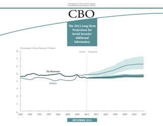
The 2013 Long-Term Projections for Social Security: Additional Information
•
2 recomendaciones•14,853 vistas


Recomendados
Recomendados
Más contenido relacionado
La actualidad más candente
La actualidad más candente (20)
Similar a The 2013 Long-Term Projections for Social Security: Additional Information
Similar a The 2013 Long-Term Projections for Social Security: Additional Information (20)
Más de Congressional Budget Office
Más de Congressional Budget Office (20)
Último
Último (20)
The 2013 Long-Term Projections for Social Security: Additional Information
- 1. CONGRESS OF THE UNITED STATES CONGRESSIONAL BUDGET OFFICE CBO The 2013 Long-Term Projections for Social Security: Additional Information Percentage of Gross Domestic Product 8 Actual Projected 7 6 Tax Revenues 5 4 Outlays 3 2 1 0 1985 1989 1993 1997 2001 2005 2009 2013 DECEMBER 2013 2017 2021 2025 2029 2033 2037
- 2. Notes and Definitions Unless otherwise noted, all years referred to are calendar years. Numbers in the text and tables may not add up to totals because of rounding. Supplemental data are posted on the Congressional Budget Office’s (CBO’s) website (www.cbo.gov/publication/44972). In this report, historical values for gross domestic product (GDP) and figures expressed as ratios to GDP reflect revised data from the national income and product accounts that were released by the Bureau of Economic Analysis on July 31, 2013. In addition, all projections incorporate those revisions. 80 percent range of uncertainty: A range of uncertainty based on 500 simulations from CBO’s long-term model. Outcomes were above the range in 10 percent of the simulations, below the range in 10 percent, and within the range in 80 percent. Median: The middle of the distribution. When the median outcome for a group of people (defined in this document by birth cohort and lifetime earnings category) is shown, the value is lower for half of the people in that group and higher for half of the group. Present value: A single number that expresses a flow of current and future income or payments in terms of an equivalent lump sum received or paid today. Summarized cost rate: The present value of outlays for a period, plus the present value of a year’s worth of benefits as a reserve at the end of the period, divided by the present value of GDP or taxable payroll over the same period. Summarized income rate: The present value of tax revenues for a period, plus the trust funds’ initial balance, divided by the present value of GDP or taxable payroll over the same period. Actuarial balance: The difference between the income rate and the cost rate. Scheduled benefits: Full benefits as calculated under current law, regardless of the amounts available in the Social Security trust funds. Payable benefits: Benefits as calculated under current law, reduced as necessary to make outlays equal the Social Security system’s revenues. Upon the exhaustion of the Social Security trust funds, the Social Security Administration would reduce all scheduled benefits such that outlays from the funds equaled revenues flowing into the funds. CBO Replacement rate: Annual benefits as a percentage of average annual lifetime earnings. Pub. No. 4796
- 3. List of Exhibits Exhibit Page The System’s Finances 1. Social Security Tax Revenues and Outlays, With Scheduled Benefits 6 2. Social Security Tax Revenues and Outlays in Selected Years, With Scheduled Benefits 7 3. Social Security Tax Revenues and Outlays, With Scheduled Benefits 8 4. Social Security Tax Revenues and Outlays, With Scheduled and Payable Benefits 9 5. Summarized Financial Measures for Social Security, With Scheduled Benefits 10 6. Trust Fund Ratio, With Scheduled Benefits 11 7. Percentage of Simulations That Show the Social Security Trust Funds Exhausted by a Particular Year 12 Distribution of Benefits 8. 14 9. Median Initial Replacement Rates for Retired Workers, With Scheduled and Payable Benefits 15 10. Median Present Value of Lifetime Benefits for Retired Workers, With Scheduled and Payable Benefits 16 11. Median Benefits and Initial Replacement Rates for Disabled Workers, With Scheduled and Payable Benefits 17 12. Percentage of Simulations in Which Payable Benefits Exceed Specified Percentages of Scheduled Benefits 18 13. Median Lifetime Social Security Taxes and Benefits, With Scheduled and Payable Benefits 19 14. CBO Median Initial Benefits for Retired Workers, With Scheduled and Payable Benefits Lifetime Social Security Benefit-to-Tax Ratios, With Scheduled and Payable Benefits 20
- 5. The 2013 Long-Term Projections for Social Security: Additional Information Social Security is the federal government’s largest single program.1 Of the 58 million people who currently receive Social Security benefits, about 70 percent are retired workers or their spouses and children, and another 11 percent are survivors of deceased workers; all of those beneficiaries receive payments through Old-Age and Survivors Insurance (OASI). The other 19 percent of beneficiaries are disabled workers or their spouses and children; they receive Disability Insurance (DI) benefits. In fiscal year 2013, Social Security’s outlays totaled $808 billion, almost one-quarter of federal spending; OASI payments accounted for about 83 percent of those outlays, and DI payments made up about 17 percent.2 Each year, CBO prepares long-term projections of revenues and outlays for the program. The most recent set of 75-year projections was published in September 2013.3 This publication presents additional information about those projections. 1. For an overview of Social Security and a discussion of the program’s financing and trust funds, see Congressional Budget Office, Social Security Policy Options (July 2010), pp. 1–5, www.cbo.gov/publication/21547. CBO Social Security has two primary sources of tax revenues: payroll taxes and income taxes on benefits. Roughly 96 percent of those revenues derive from a payroll tax—generally, 12.4 percent of earnings— that is split evenly between workers and their employers; self-employed people pay the entire tax.4 The payroll tax applies only to taxable 2. Numbers for 2013 were derived from information reported in Department of the Treasury, Final Monthly Treasury Statement of Receipts and Outlays of the United States Government for Fiscal Year 2013 Through September 30, 2013, and Other Periods (October 2013), www.fms.treas.gov/mts/mts0913.pdf. 3. See Congressional Budget Office, The 2013 Long-Term Budget Outlook (September 2013), www.cbo.gov/ publication/44521. Some of the 75-year projections in that volume extended through fiscal year 2088 because CBO generally considers the projection period to begin in the next fiscal year (in this case, fiscal year 2014). In this report and in Chapter 3 (“Social Security”) of The 2013 Long-Term Budget Outlook, the 75-year projection period consists of calendar years 2013 through 2087, matching the period used in Social Security Administration, The 2013 Annual Report of the Board of Trustees of the Federal Old-Age and Survivors Insurance and Federal Disability Insurance Trust Funds (May 2013), www.ssa.gov/oact/tr/ 2013/index.html. earnings—earnings up to a maximum annual amount ($113,700 in 2013). The remaining share of tax revenues—4 percent—is collected from income taxes that higher-income beneficiaries pay on their benefits. Revenues credited to the program totaled $745 billion in fiscal year 2013. Revenues from taxes, along with intragovernmental interest payments, are credited to Social Security’s two trust funds—one for OASI and one for DI—and the program’s benefits and administrative costs are paid from those funds. Although legally separate, the funds often are described collectively as the OASDI trust funds. In a given year, the sum of receipts to a fund along with the interest that is credited on balances, minus spending for benefits and administrative costs, constitutes that fund’s surplus or deficit. 4. The worker’s portion of the payroll tax was reduced by 2 percentage points for 2011 and 2012 (as was the tax on the self-employed), and the reduction in tax revenues was made up by reimbursements from the U.S. Treasury’s general fund. In this report, Social Security tax revenues include those reimbursements.
- 6. THE 2013 LONG-TERM PROJECTIONS FOR SOCIAL SECURITY: ADDITIONAL INFORMATION In calendar year 2010, for the first time since the enactment of the Social Security Amendments of 1983, annual outlays for the program exceeded annual tax revenues (that is, outlays exceeded total revenues excluding interest credited to the trust funds). In 2012, outlays exceeded noninterest income by about 7 percent, and CBO projects that the gap will average about 12 percent of tax revenues over the next decade. As more members of the baby-boom generation retire, outlays will increase relative to the size of the economy, whereas tax revenues will remain at an almost constant share of the economy. As a result, the gap will grow larger in the 2020s and will exceed 30 percent of revenues by 2030. CBO projects that under current law, the DI trust fund will be exhausted in fiscal year 2017, and the OASI trust fund will be exhausted in 2033. If a trust fund’s balance fell to zero and current revenues were insufficient to cover the benefits specified in law, the Social Security Administration would no longer have legal authority to pay full benefits when they were due. In 1994, legislation redirected revenues from the OASI trust fund to prevent the imminent exhaustion of the DI trust fund. In part because of that experience, it is a common analytical convention to consider the DI and OASI trust funds as combined. Thus, CBO projects, if some future legislation shifted resources from the OASI trust fund to the DI trust fund, the combined OASDI trust funds would be exhausted in 2031. The amount of Social Security taxes paid by various groups of people differs, as do the benefits that different groups receive. For example, people with higher earnings pay more in Social Security payroll CBO taxes than do lower-earning participants, and they also receive benefits that are larger (although not proportionately so). Because Social Security’s benefit formula is progressive, replacement rates— annual benefits as a percentage of average annual lifetime earnings—are lower, on average, for workers who have had higher earnings. As another example, the amount of taxes paid and benefits received will be greater for people who were born more recently because they typically will have higher earnings over a lifetime, even after an adjustment for inflation, CBO projects. Scheduled and Payable Benefits CBO prepares two types of benefit projections. Benefits as calculated under the Social Security Act, regardless of the balances in the trust funds, are called scheduled benefits. However, if the trust funds were depleted, the Social Security Administration would no longer have legal authority to pay full benefits when they were due. If that were to occur, annual outlays would be limited to annual revenues in the years after the exhaustion of the trust funds.5 Benefits thus reduced are called payable benefits. In such a case, all receipts to the trust funds would be used, and the trust fund balances would remain essentially at zero. When presenting projections of Social Security’s finances, CBO 5. See Christine Scott, Social Security: What Would Happen if the Trust Funds Ran Out? Report for Congress RL33514 (Congressional Research Service, October 2013), www.fas.org/sgp/crs/misc/RL33514.pdf. As explained in that report, it is unclear how payments would be reduced. In its analysis, CBO assumes that each year after the trust funds became exhausted, each individual’s annual benefit would be reduced by the percentage necessary for outlays to match revenues. generally focuses on scheduled benefits because, by definition, the system would be fully financed if payable benefits were all that was disbursed. Quantifying Uncertainty To quantify the uncertainty in its Social Security projections, CBO, using its long-term model, created a distribution of outcomes from 500 simulations. In those simulations, the values for most of the key demographic and economic factors that underlie the analysis—for example, fertility and mortality rates, interest rates, and the rate of growth of productivity—were based on historical patterns of variation.6 Several exhibits in this publication show the simulations’ 80 percent range of uncertainty: That is, in 80 percent of the 500 simulations, the value in question fell within the range shown; in 10 percent of the simulations, the value was above that range; and in 10 percent, it was below. Long-term projections are necessarily uncertain, and that uncertainty is illustrated in this publication; nevertheless, under a variety of values for key factors, the general conclusions of this analysis are unchanged. In contrast to previous reports, the uncertainty analysis in this year’s report focuses on the next 25 years. Beyond that period, the projected ratio of debt held by the public to gross domestic product (GDP) is well outside historical 6. For more information, see Congressional Budget Office, Quantifying Uncertainty in the Analysis of Long-Term Social Security Projections (November 2005), www.cbo.gov/ publication/17472. The methodology used in this report differs slightly from the techniques described in that earlier publication. This year, CBO updated the data used in the time-series equations. 2
- 7. THE 2013 LONG-TERM PROJECTIONS FOR SOCIAL SECURITY: ADDITIONAL INFORMATION experience in a significant share of simulations. Projections of economic outcomes under those circumstances are unreliable, precluding analysis of the uncertainty of those outcomes. Changes in CBO’s Long-Term Social Security Projections Since 2012 The shortfalls for Social Security that CBO is currently projecting are larger than those the agency projected a year ago.7 Spending and Revenues Measured Relative to Taxable Payroll. The 75-year imbalance has increased from 1.95 percent to 3.36 percent of taxable payroll (see Exhibit 5). The higher projection results from a number of factors, including increases in projections of life expectancy and of the disability incidence rate, both of which raise projected outlays for benefits, and decreases in the projection of income taxes on benefits. This year, rather than using the Social Security trustees’ projections of life expectancy (as done for earlier analyses), CBO used its own, which incorporate faster growth of that measure than the Social Security trustees anticipate. In addition, CBO increased its projection of the share of workers who will receive Social Security disability benefits, resulting in higher projected spending for Social Security.8 Of the 1.4 percentage-point increase in the 75-year imbalance, a higher projection of life expectancy accounts for 0.6 percentage points, a higher projec7. See Congressional Budget Office, The 2012 Long-Term Projections for Social Security: Additional Information (October 2012), www.cbo.gov/publication/43648. 8. For further details on CBO’s projections of life expectancy and disability incidence, see Congressional Budget Office, The 2013 Long-Term Budget Outlook (September 2013), pp. 104–107, www.cbo.gov/publication/44521. CBO tion of the disability incidence rate accounts for 0.1 percentage point, reductions in income tax rates enacted in January 2013 (which reduce the revenues for Social Security from income taxes on benefits) account for 0.4 percentage points, and other factors (including a projection period that extends a year later and updated data) account for 0.4 percentage points. When measured as a share of taxable payroll, longterm tax revenues are lower than those that CBO projected in 2012, but long-term outlays are higher. Compared with last year’s projection, the 75-year income rate—a measure of Social Security’s tax revenues—is 0.3 percentage points lower because revenues from income taxes on benefits are now projected to be lower as a result of the American Taxpayer Relief Act of 2012.9 The 75-year cost rate—a measure of outlays—is 1.1 percentage points higher. Outlays are a higher share of taxable payroll because of the increases in projections of life expectancy and the incidence of disability. Spending and Revenues Measured Relative to GDP. When measured as a share of GDP, the projection of the income rate is slightly lower than it was in last year’s report. CBO reduced its projection of how much a new excise tax on some employmentbased health insurance plans with premiums above a certain threshold will affect the mix of compensation that employees receive, resulting in a lower projection of taxable earnings. That reduc9. The income rate is the present value of tax revenues for a period, plus the trust funds’ initial balance, divided by the present value of GDP or taxable payroll over the same period. The cost rate is the present value of outlays for a period, plus the present value of a year’s worth of benefits as a reserve at the end of the period, divided by the present value of GDP or taxable payroll over the same period. tion in taxable earnings was partly offset by a lower projection of growth in health care costs, which implies that a larger share of compensation will be paid as taxable earnings, rather than nontaxable health benefits. As a result of those partially offsetting changes, CBO projects that taxable earnings will make up a smaller share of compensation than the amount estimated last year. Together with the reductions in income tax rates, those changes imply that the income rate will be slightly lower than the level estimated last year.10 The current projection of Social Security spending as a percentage of GDP is lower than last year’s projection through 2028—for much of that period, almost entirely because of revisions to GDP.11 For years after 2028, Social Security spending as a percentage of GDP is higher than or equal to the amounts CBO projected last year, and the difference is greater if the amounts projected in last year’s report are adjusted to incorporate revised values for GDP. The higher projection results from the same factors that increase costs as a share of taxable payroll, including increases in projections of life expectancy and the disability incidence rate. The 75-year imbalance is greater as a share of GDP for the same reasons that it is greater as a share of taxable payroll. The imbalance rose from 0.73 percent of GDP to 1.17 percent. 10. See Congressional Budget Office, The 2013 Long-Term Budget Outlook (September 2013), p. 105, www.cbo.gov/ publication/44521. 11. In this report, historical values for GDP and figures expressed as ratios to GDP reflect revised data from the national income and product accounts that were released by the Bureau of Economic Analysis on July 31, 2013. In addition, all projections incorporate those revisions. 3
- 8. THE 2013 LONG-TERM PROJECTIONS FOR SOCIAL SECURITY: ADDITIONAL INFORMATION Related CBO Analyses Further information about Social Security and CBO’s projections is available in other CBO publications: Various approaches to changing the program are presented in Social Security Policy Options (July 2010), www.cbo.gov/publication/21547, and in Policy Options for the Social Security Disability Insurance Program (July 2012), www.cbo.gov/ publication/43421. The current long-term projections are consistent with the 10-year baseline CBO published in Updated Budget Projections: Fiscal Years 2013 to 2023 (May 2013), www.cbo.gov/publication/ 44172. Data in that report and in The 2013 LongTerm Budget Outlook (September 2013), CBO www.cbo.gov/publication/44521, generally are presented for fiscal years; this analysis, Social Security Policy Options, and Policy Options for the Social Security Disability Insurance Program use calendar year data. The current projections update those published in The 2012 Long-Term Projections for Social Security: Additional Information (October 2012), www.cbo.gov/publication/43648. Differences in the two sets of projections result from newly available economic and programmatic data, updated assumptions about future demographic and economic trends, and improvements in models. The methodology used to develop the projections in this publication is described in CBO’s Long-Term Model: An Overview (June 2009), www.cbo.gov/ publication/20807. The data underlying the figures in this report and expanded versions of some of the tables are available as supplemental material on CBO’s website (www.cbo.gov/publication/44972). The values used for the demographic and economic variables underlying the projections, are explained in a section, “CBO’s Projections of Demographic and Economic Trends,” in Chapter 1 of The 2013 Long-Term Budget Outlook (pp. 15–21). Numerous other aspects of the program are addressed in various publications available on the “Retirement” page of CBO’s website (www.cbo.gov/topics/retirement). 4
- 9. The System’s Finances The first part of this publication (Exhibits 1 through 7) examines Social Security’s financial status from several vantage points. The fullest perspective is provided by projected streams of annual revenues and outlays. A more succinct analysis is given by measures that summarize the annual streams in a single number. The system’s finances also are described by projecting the trust fund ratio, the amount in the trust funds at the beginning of a year in proportion to the outlays in that year. CBO
- 10. THE SYSTEM’S FINANCES THE 2013 LONG-TERM PROJECTIONS FOR SOCIAL SECURITY: ADDITIONAL INFORMATION Exhibit 1. In 2012, Social Security’s total outlays (benefits plus administrative costs) equaled 4.9 percent of the country’s gross domestic product; tax revenues dedicated to the program equaled 4.5 percent of GDP. Most of Social Security’s tax revenues come from payroll taxes, although a small portion comes from income taxes on benefits paid to higherincome beneficiaries. In addition to those tax revenues, the trust funds are credited with interest on the Treasury securities they hold. Social Security Tax Revenues and Outlays, With Scheduled Benefits (Percentage of gross domestic product) 7 Actual Projected 6 Tax Revenues a 5 4 Outlays b 3 2 1 0 1985 Source: 1991 1997 2003 2009 2015 2021 2027 2033 2039 2045 2051 2057 2063 2069 2075 2081 2087 Congressional Budget Office. a. Includes payroll taxes, income taxes on benefits, and, in 2011 and 2012, reimbursements from the U.S. Treasury’s general fund to make up for reductions in payroll taxes in those years. b. Includes scheduled benefits and administrative costs. During the next few decades, the number of beneficiaries will increase as the baby-boom generation ages. In 2037, scheduled spending will be 6.3 percent of GDP, CBO estimates. Over the ensuing decade, spending will decline slightly, relative to the size of the economy, as people in the baby-boom generation die. Demographers generally predict that life expectancy will continue to rise and that birth rates will remain as they are now, so scheduled outlays are projected to resume their upward trajectory around 2050, reaching 6.7 percent of GDP in 2087. The amount of tax revenues credited to the trust funds is projected to be about 4.4 percent of GDP through 2016. Tax revenues are then projected to slowly increase, reaching about 4.7 percent of GDP by the late 2020s. In the decades that follow, tax revenues are projected to decline slightly relative to GDP, to 4.6 percent by the late 2060s. Three factors are important in creating that pattern. CBO expects that health care costs will continue to rise more rapidly than taxable earnings, a trend that by itself would decrease the proportion of compensation that workers receive as taxable (Continued) CBO 6
- 11. THE SYSTEM’S FINANCES THE 2013 LONG-TERM PROJECTIONS FOR SOCIAL SECURITY: ADDITIONAL INFORMATION Exhibit 2. Social Security Tax Revenues and Outlays in Selected Years, With Scheduled Benefits (Percentage of gross domestic product) Actual, 2012 Tax Revenues Outlays Difference Source: Note: 4.53 4.86 -0.33 Projected 2062 2037a 4.66 (4.5 to 4.9) 6.27 (5.6 to 7.3) -1.61 (-2.5 to -1.1) b 2087 4.66 6.41 -1.74 4.63 6.74 -2.11 Congressional Budget Office. Tax revenues consist of payroll taxes and income taxes on benefits that are credited to the Social Security trust funds in the specified year. In 2011 and 2012, they include reimbursements from the U.S. Treasury’s general fund to make up for reductions in payroll taxes in those years. Outlays consist of scheduled benefits and administrative costs; scheduled benefits are benefits as calculated under the Social Security Act, regardless of the balances in the trust funds. a. The range spans the outcomes of 80 percent of CBO’s simulations. Beyond 2037, the projected ratio of debt held by the public to GDP is well outside historical experience in a significant share of simulations. Projections of economic outcomes under those circumstances are unreliable, precluding analysis of the uncertainty of those outcomes. b. The range of differences displayed does not equal the difference between the outlays and revenues shown because each value is drawn from a different simulation. (Continued) earnings. However, the Affordable Care Act imposed an excise tax on some employment-based health insurance plans that have premiums above a specified threshold. Some employers and workers will respond to that tax—which is scheduled to take effect in 2018—by shifting to less expensive plans, thereby reducing the share of compensation composed of health insurance premiums and increasing the share composed of taxable earnings. CBO projects that the effects of the excise tax on the mix of compensation will roughly offset the effects of rising costs for health care for a few decades; thereafter, the impact of rising health care costs will outweigh the impact of the tax. In addition, when the distribution of earnings widens, as it has in recent decades, the taxable share of earnings declines because more earnings are above the maximum amount that is taxed for Social Security. CBO projects that the distribution of earnings will widen somewhat during the next few decades. As a result of a combination of those three factors, the share of compensation that workers receive as taxable earnings is projected to remain close to 81 percent until around 2050 and then decline slightly. With outlays increasing sharply and tax revenues rising only slightly (both relative to GDP), the difference between them is projected to increase from about -0.3 percent of GDP in 2012 to about -1.6 percent in 2037. In 10 percent of CBO’s simulations, that difference is larger than -2.5 percent of GDP, and in 10 percent, it is smaller than -1.1 percent. The gap widens further beyond 2037, in part because life expectancy is expected to continue to rise. CBO 7
- 12. THE SYSTEM’S FINANCES THE 2013 LONG-TERM PROJECTIONS FOR SOCIAL SECURITY: ADDITIONAL INFORMATION Exhibit 3. The uncertainty in CBO’s projections is illustrated by the range of outcomes from a series of 500 simulations in which most of the key demographic and economic factors that underlie the analysis were varied on the basis of historical patterns. In this year’s report, outcomes for the range of uncertainty stop in 2037 (thus focusing on the next 25 years because, in later years, the projected ratio of debt held by the public to GDP is well outside historical experience in a significant share of simulations, making projections of economic outcomes unreliable and precluding analysis of the uncertainty of those outcomes). Social Security Tax Revenues and Outlays, With Scheduled Benefits (Percentage of gross domestic product) 8 Actual Projected 7 6 Tax Revenuesa 5 4 Outlaysb 3 2 1 0 1985 1989 1993 1997 2001 2005 2009 2013 2017 2021 2025 2029 2033 2037 Source: Congressional Budget Office. Note: The lines indicate CBO’s projections of expected outcomes. The shaded areas indicate the 80 percent range of uncertainty. Beyond 2037, the projected ratio of debt held by the public to GDP is well outside historical experience in a significant share of simulations. Projections of economic outcomes under those circumstances are unreliable, precluding analysis of the uncertainty of those outcomes. a. Includes payroll taxes, income taxes on benefits, and, in 2011 and 2012, reimbursements from the U.S. Treasury’s general fund to make up for reductions in payroll taxes in those years. b. Includes scheduled benefits and administrative costs. CBO CBO projects that Social Security tax revenues will equal 4.7 percent of GDP in 2037, but in 10 percent of the simulations, tax revenues in 2037 are less than 4.5 percent of GDP, and in 10 percent, they exceed 4.9 percent. The range of uncertainty for Social Security outlays is wider than that for revenues. CBO projects that if benefits are paid as scheduled, outlays will equal 6.3 percent of GDP in 2037, but in 10 percent of the simulations, outlays that year are less than 5.6 percent of GDP, and in 10 percent, they exceed 7.3 percent. In most cases, outlays in 2037 account for a much larger share of GDP than the 4.8 percent estimated for 2013. Uncertainty surrounding projections for Social Security revenues and outlays over the next 25 years largely derives from uncertainty in mortality rates and productivity growth. The former has the largest effect on benefits, as life spans determine the number of years people receive benefits. The latter affects total earnings and, hence, tax revenues, benefits, and GDP, but the ratio of tax revenues to GDP does not change much even as the growth of productivity changes. Because earnings growth affects benefits with a lag, uncertainty about that growth has a greater effect on the future ratio of outlays to GDP. 8
- 13. THE SYSTEM’S FINANCES THE 2013 LONG-TERM PROJECTIONS FOR SOCIAL SECURITY: ADDITIONAL INFORMATION Exhibit 4. If the projected gap between outlays and revenues occurred, it would ultimately eliminate the balance in the trust funds. Once the balance was depleted, the Social Security Administration would no longer have legal authority to pay full benefits when they were due. Annual outlays would be limited to annual revenues in the years after the exhaustion of the trust funds. (As explained in a report by the Congressional Research Service, how payments would be reduced is unclear. See Christine Scott, Social Security: What Would Happen if the Trust Funds Ran Out? Report for Congress RL33514 [Congressional Research Service, October 2013], www.fas.org/sgp/crs/misc/RL33514.pdf.) Social Security Tax Revenues and Outlays, With Scheduled and Payable Benefits (Percentage of gross domestic product) 7 Actual Projected 6 Outlays With Scheduled Benefits b a Tax Revenues 5 Outlays With Payable Benefits 4 Outlays b b 3 2 1 0 1985 Source: 1991 1997 2003 2009 2015 2021 2027 2033 2039 2045 2051 2057 2063 2069 2075 2081 2087 Congressional Budget Office. a. Includes payroll taxes, income taxes on benefits, and, in 2011 and 2012, reimbursements from the U.S. Treasury’s general fund to make up for reductions in payroll taxes in those years. Tax revenues shown are consistent with payable benefits; they would be slightly higher if scheduled benefits were paid because revenues from income taxes paid on those benefits would be higher. b. Includes benefits and administrative costs. In its analysis, CBO assumes that each year after the trust funds became exhausted, each individual’s annual benefit would be reduced by the percentage necessary for outlays to match revenues. Payable benefits would equal scheduled benefits until the trust funds were exhausted; after that, they would equal the Social Security program’s annual revenues. CBO projects that the trust funds, considered in combination for analytical purposes, will be exhausted in 2031. (For the DI trust fund, that date is fiscal year 2017; and for the OASI trust fund, 2033.) For 2032, revenues are projected to equal 75 percent of scheduled outlays. Thus, payable benefits will be 25 percent less than scheduled benefits. For more than 20 years thereafter, the gap between scheduled and payable benefits will fluctuate narrowly around 26 percent. It will then widen, and by 2087, payable benefits will be 34 percent smaller than scheduled benefits. CBO 9
- 14. THE SYSTEM’S FINANCES THE 2013 LONG-TERM PROJECTIONS FOR SOCIAL SECURITY: ADDITIONAL INFORMATION Exhibit 5. Summarized Financial Measures for Social Security, With Scheduled Benefits As a Percentage of Gross Domestic Product Actuarial Income Cost Balance Rate Rate (Difference) 25 years (2013–2037) 50 years (2013–2062) 75 years (2013–2087) Source: Note: 5.22 4.98 4.89 5.75 5.93 6.07 -0.53 -0.95 -1.17 As a Percentage of Taxable Payroll Actuarial Income Cost Balance Rate Rate (Difference) 14.90 14.17 14.00 16.41 16.87 17.35 -1.51 -2.69 -3.36 Congressional Budget Office. Over the relevant periods, the income rate is the present value of annual tax revenues plus the initial trust fund balance, and the cost rate is the present value of annual outlays plus the present value of a year’s worth of benefits as a reserve at the end of the period, each divided by the present value of GDP or taxable payroll. The actuarial balance is the difference between the income and cost rates. To present the results of long-term projections succinctly, analysts often summarize scheduled outlays and revenues as a single number that covers a given period (for example, total outlays over 75 years). The data are summarized by computing the present value of outlays or tax revenues for a period and dividing that figure by the present value of GDP or taxable payroll over the same period. (Present value is a single number that expresses a flow of current and future income, or payments, in terms of an equivalent lump sum received or paid today—in this case, applying the interest rate used to compute interest credited to the trust funds.) The income rate is the present value of annual noninterest revenues plus the initial trust fund balance, and the cost rate is the present value of annual outlays plus a target trust fund balance at the end of the period (which is traditionally the following year’s projected outlays), each divided by the present value of GDP or taxable payroll. The actuarial balance is the difference between the income and cost rates. The estimated 75-year actuarial balance is -1.17 percent of GDP or -3.36 percent of taxable payroll. That means, for example, that if the Social Security payroll tax rate was increased immediately and permanently by 3.36 percentage points— from the current rate of 12.40 percent to 15.76 percent—or if scheduled benefits were reduced by an equivalent amount, then the trust funds’ projected balance at the end of 2087 would equal projected outlays for 2088. Because, relative to GDP, the gap between projected costs and projected revenues is widening over time, the actuarial balance is more negative over 75 years than over shorter periods. CBO 10
- 15. THE SYSTEM’S FINANCES THE 2013 LONG-TERM PROJECTIONS FOR SOCIAL SECURITY: ADDITIONAL INFORMATION Exhibit 6. The trust fund ratio—the balance in the Social Security trust funds at the beginning of the year divided by the system’s outlays for that year— indicates the proportion of a year’s cost that could be paid with the funds available. The trust fund ratio for 2012 was 3.4, and CBO projects that it will fall to 3.3 this year. The rate of decline will accelerate in subsequent decades, and the ratio will reach zero in 2032; that is, the trust funds (combined) will be exhausted by the end of 2031, CBO projects. At that point, payments to current and new beneficiaries would need to be reduced to make the outlays equal revenues. Trust Fund Ratio, With Scheduled Benefits 4 Actual Projected 3 2 1 0 -1 -2 -3 1985 1989 Source: Congressional Budget Office. 1993 1997 2001 2005 2009 2013 2017 2021 2025 2029 2033 2037 Notes: The trust fund ratio is the ratio of the trust fund balance (the amount in the trust funds) at the beginning of a year to outlays in that year. Outlays consist of benefits and administrative costs. The trust ratio reaches zero the year following trust fund exhaustion. Under current law, the trust funds cannot incur negative balances. The negative balances shown in this exhibit indicate a projected shortfall, reflecting the trust funds’ inability to pay scheduled benefits out of current-law revenues. The dark line indicates CBO’s projection of expected outcomes; the shaded area indicates the 80 percent range of uncertainty around the projection. Beyond 2037, the projected ratio of debt held by the public to GDP is well outside historical experience in a significant share of simulations. Projections of economic outcomes under those circumstances are unreliable, precluding analysis of the uncertainty of those outcomes. The year in which the trust funds are exhausted could differ significantly from CBO’s projection, however. In CBO’s simulations, in which most of the key demographic and economic factors in the analysis were varied on the basis of historical patterns, the trust fund ratio falls to zero in 2029 or earlier (that is, the trust funds are exhausted in 2028 or earlier) 10 percent of the time; the ratio drops to zero in 2037 or later (that is, the trust funds are exhausted in 2036 or later) another 10 percent of the time. (The shaded area in the figure shows the 80 percent range of uncertainty. The intersection between the shaded area and the horizontal line at zero, spanning the years between 2029 and 2037, corresponds to the 80 percent range of uncertainty about the year in which the trust fund ratio falls to zero.) The negative balances represent CBO’s estimates of the cumulative amount of scheduled benefits, plus interest on debt incurred to pay those benefits, that cannot be paid from the program’s revenues under current law, expressed as a ratio to outlays in each year. By 2036, that shortfall amounts to more than one year’s worth of benefits. CBO 11
- 16. THE SYSTEM’S FINANCES THE 2013 LONG-TERM PROJECTIONS FOR SOCIAL SECURITY: ADDITIONAL INFORMATION Exhibit 7. An alternative way to consider uncertainty is to examine the percentage of simulations in which the trust funds are exhausted by a specific year. In those simulations, most of the key demographic and economic factors that underlie the analysis were varied on the basis of historical patterns. In 10 percent of CBO’s simulations, the funds combined are exhausted by 2028, and in 42 percent, they are exhausted by 2030. In 94 percent of the simulations, the trust funds are exhausted by 2037. CBO’s best estimate is that they will be exhausted in 2031. Percentage of Simulations That Show the Social Security Trust Funds Exhausted by a Particular Year 100 90 80 70 60 50 40 30 20 10 0 2013 Source: Note: CBO 2015 2017 2019 2021 2023 2025 2027 2029 2031 2033 2035 2037 Congressional Budget Office. The data are based on 500 simulations from CBO’s long-term model. Beyond 2037, the projected ratio of debt held by the public to GDP is well outside historical experience in a significant share of simulations. Projections of economic outcomes under those circumstances are unreliable, precluding analysis of the uncertainty of those outcomes. 12
- 17. Distribution of Benefits In the second part of this publication (Exhibits 8 through 14), CBO examines the program’s effects on people by grouping Social Security participants according to various characteristics and presenting the average taxes and benefits for those groups. In its analysis, CBO divided people into groups by the decade in which they were born and by the quintile of their lifetime household earnings.1 For example, one 10-year cohort consists of people born in the 1940s, and the highest earnings quintile consists of the top fifth of earners. CBO’s modeling approach produces estimates for individuals; household status is used only to place people into earnings groups. In this part of the analysis, benefits are calculated net of income taxes paid on benefits by higherincome recipients and credited to the Social Security trust funds.2 The payroll taxes paid do not reflect the 2 percentage-point reduction in 2011 and 2012. Median values are estimated for each group: Estimates for half of the people in the group are lower, and estimates for half are higher. Most retired and disabled workers receive Social Security benefits on the basis of their own work history. In Exhibits 8 through 11, this publication presents measures of those benefits that do not include benefits received by dependents or survivors who are entitled to them on the basis of another person’s work history. Exhibit 12 shows the percentage of simulations in which payable benefits exceed specified percentage of scheduled benefits. For a more comprehensive perspective on the distribution of Social Security benefits, Exhibits 13 and 14 present measures of the total amount of Social Security payroll taxes that each participant pays over his or her lifetime as well as the total Social Security benefits—including payments received as a worker’s dependent or as a survivor—that each receives over a lifetime. 1. Each person who lives at least to age 45 is ranked by lifetime household earnings. Lifetime earnings for someone who is single in all years equal the present value of his or her real (inflationadjusted) earnings over a lifetime. In any year that a person is married, the earnings measure is a function of his or her earnings plus those of his or her spouse (adjusted for economies of scale in household consumption). To compute present values in Social Security analyses, CBO uses a real discount rate of 3.0 percent, which equals the long-term rate used to compute interest for the Social Security trust funds. 2. Some of the income taxes collected on Social Security benefits are credited to Medicare’s Hospital Insurance trust fund. In this analysis, Social Security benefits are not reduced by that portion of those income taxes. CBO
- 18. DISTRIBUTION OF BENEFITS THE 2013 LONG-TERM PROJECTIONS FOR SOCIAL SECURITY: ADDITIONAL INFORMATION Exhibit 8. Median Initial Benefits for Retired Workers, With Scheduled and Payable Benefits (Thousands of 2013 dollars) 10-Year Birth Cohort All Retired Workers Scheduled Payable Lowest Quintile of Lifetime Household Earnings Scheduled Payable Middle Quintile of Lifetime Household Earnings Scheduled Payable Highest Quintile of of Lifetime Household Earnings Scheduled Payable All 1940s 1960s 1980s 2000s 17 19 22 29 17 17 16 20 9 11 13 18 9 10 10 13 1940s 1960s 1980s 2000s 22 22 25 34 22 21 19 24 11 12 14 19 19 20 23 32 11 11 11 13 19 19 18 22 25 30 38 51 25 28 29 36 23 23 26 36 23 22 20 25 27 32 40 54 27 30 31 38 14 17 21 29 14 16 16 20 19 26 32 44 19 24 25 31 Men Women 1940s 1960s 1980s 2000s Source: Note: 13 16 19 26 13 15 14 18 8 10 12 17 8 10 9 12 Congressional Budget Office. Initial annual benefits are computed for all individuals who are eligible to claim retirement benefits at age 62 and who have not yet claimed any other benefit. All workers are assumed to claim benefits at age 65. All values are net of income taxes paid on benefits and credited to the Social Security trust funds. Future retired workers are projected to receive higher initial scheduled Social Security benefits than today’s beneficiaries receive (net of income taxes paid on the benefits and credited to the Social Security trust funds, and adjusted for the effects of inflation). CBO considered a hypothetical benefit amount: the median initial benefit among workers if everyone claimed benefits at age 65, based on earnings through age 61. The median initial scheduled benefit rises over time because of growth in average earnings. However, the effect of growing earnings will be partly offset for several cohorts by the scheduled rise in the full retirement age, from 65 for people born before 1938 to 67 for those born after 1959. The effect is equivalent to a reduction in benefits at any age at which benefits are claimed. Once the older retirement age is in place, the median initial benefit will grow at about the same rate as median earnings. When the trust funds are exhausted, payable benefits will fall, but then they will rise again as earnings (and therefore tax revenues) grow. Initial payable benefits, measured in 2013 dollars, are lower than initial scheduled benefits for people born in the latter part of the 1960s and later. Projected benefits are lower for women than for men in all cohorts (because women have lower average earnings), although the gap narrows (as a share of men’s benefits) for later cohorts as men’s and women’s earnings become more equal. For the 1940s cohort, projected initial benefits for women are about 40 percent below those for men, but for the 1970s cohort and later groups, they are about 25 percent below those for men. CBO 14
- 19. DISTRIBUTION OF BENEFITS THE 2013 LONG-TERM PROJECTIONS FOR SOCIAL SECURITY: ADDITIONAL INFORMATION Exhibit 9. Median Initial Replacement Rates for Retired Workers, With Scheduled and Payable Benefits (Percent) 10-Year Birth Cohort All Retired Workers Scheduled Payable Lowest Quintile of Lifetime Household Earnings Scheduled Payable Middle Quintile of Lifetime Household Earnings Scheduled Payable Highest Quintile of of Lifetime Household Earnings Scheduled Payable All 1940s 1960s 1980s 2000s 46 43 46 45 46 41 35 31 77 71 74 73 77 65 57 51 45 42 44 43 45 40 33 30 32 27 28 26 32 26 22 19 40 39 42 40 40 38 31 28 26 22 23 22 26 21 18 15 52 45 47 46 52 43 36 32 42 35 36 35 42 33 27 24 Men 1940s 1960s 1980s 2000s 41 40 43 42 41 38 32 29 65 66 69 67 65 61 53 47 1940s 1960s 1980s 2000s 54 47 51 49 54 45 38 34 83 76 77 76 83 67 58 53 Women Source: Note: CBO Congressional Budget Office. The initial replacement rate is a worker’s initial benefit as a percentage of a worker’s average annual lifetime earnings. (To compute lifetime earnings, past earnings are adjusted for average growth in economywide earnings.) Replacement rates are computed for all individuals who are eligible to claim retirement benefits at age 62 and who have not yet claimed any other benefit. All workers are assumed to claim benefits at age 65. All values are net of income taxes paid on benefits and credited to the Social Security trust funds. Initial replacement rates—initial annual benefits net of income taxes paid to the Social Security trust funds on those benefits as a percentage of average annual lifetime earnings—provide a perspective on retired workers’ benefits that is different from that provided by looking simply at dollar amounts. Several factors affect the patterns. First, the progressive nature of Social Security’s benefit formula results in replacement rates that are higher for workers within a birth cohort who have had lower earnings. Second, with payable benefits, the replacement rate will drop noticeably at all earnings amounts for people in the cohorts that first receive benefits after the trust funds are exhausted. Third, the scheduled increase in the full retirement age will, in the absence of other changes, lower the replacement rate for future beneficiaries (for any chosen age for claiming benefits) compared with the rate for people who are claiming benefits now. However, because of other factors, such as changes in the relative earnings of different groups, overall median replacement rates with scheduled benefits for the cohorts shown in the exhibit do not vary much. People in later cohorts, however, are expected to collect benefits for a longer time as life expectancy increases. Fourth, because women tend to have lower lifetime earnings, their average replacement rates are higher than men’s are, especially for earlier birth cohorts. The difference between the rates for women and men is largest in the highest quintile, in part because that group includes many women who spend time out of the labor force or who work part time. In contrast, most men in households with high earnings are employed full time. 15
- 20. DISTRIBUTION OF BENEFITS THE 2013 LONG-TERM PROJECTIONS FOR SOCIAL SECURITY: ADDITIONAL INFORMATION Exhibit 10. Median Present Value of Lifetime Benefits for Retired Workers, With Scheduled and Payable Benefits (Thousands of 2013 dollars) 10-Year Birth Cohort All Retired Workers Scheduled Payable Lowest Quintile of Lifetime Household Earnings Scheduled Payable Middle Quintile of Lifetime Household Earnings Scheduled Payable Highest Quintile of of Lifetime Household Earnings Scheduled Payable All 1940s 1960s 1980s 2000s 191 226 282 410 188 183 206 278 95 114 153 229 94 95 111 155 211 256 316 463 207 206 232 313 328 415 547 774 324 331 404 536 260 281 347 498 258 227 255 335 378 465 620 863 372 368 457 601 171 231 293 432 168 185 213 290 254 349 447 652 249 278 328 448 Men 1940s 1960s 1980s 2000s 231 250 311 447 230 203 227 304 103 117 160 236 102 97 117 162 1940s 1960s 1980s 2000s 161 207 260 378 158 168 190 257 87 112 147 220 86 94 106 149 Women Source: Note: CBO Congressional Budget Office. Benefits are the present value of all retired-worker benefits received. To calculate their present value, benefits are adjusted for inflation (to produce constant dollars) and discounted to age 62. All values are net of income taxes paid on benefits and credited to the Social Security trust funds. CBO calculates lifetime retirement benefits as the present value, discounted to the year in which the beneficiary turns 62, of all such benefits that a worker receives from the program. CBO estimates that real median lifetime scheduled benefits for each birth cohort will be greater than those for the preceding cohort, because benefits increase with earnings, real earnings are expected to continue to rise over time, and each cohort is projected to live longer than the previous one. For example, real median scheduled lifetime benefits for people born in the 2000s will be more than twice those for people born in the 1940s; real median payable lifetime benefits for the 2000s cohort will be about one-and-a-half times as large. The projected trends in median lifetime retirement benefits differ from the trends in median initial benefits for two reasons. First, as life expectancy increases, people will collect benefits for longer periods, so lifetime scheduled benefits will grow faster than initial scheduled benefits. Second, although cohorts that begin to receive benefits before the trust funds are exhausted will collect their initial scheduled benefits, some members of those cohorts will still be receiving benefits when the trust funds are exhausted. At that point, payable benefits will be less than scheduled benefits, and the lifetime payable benefits for those recipients will be less than their lifetime scheduled benefits. Hence, for people born in the 1940s and 1960s, the difference between initial scheduled and payable benefits is smaller than the difference between lifetime scheduled and payable benefits. Most of those individuals begin receiving benefits before the trust funds are exhausted, so initial scheduled and payable benefits are the same. In contrast, for people born in the 1980s, payable benefits are smaller than scheduled benefits in all years, and the reductions in initial and lifetime benefits are similar. Lifetime benefits are lower for women than for men, although the gap is smaller than it is for initial benefits because women live longer, on average, and thus tend to collect benefits for a longer time. 16
- 21. DISTRIBUTION OF BENEFITS THE 2013 LONG-TERM PROJECTIONS FOR SOCIAL SECURITY: ADDITIONAL INFORMATION Exhibit 11. Median Benefits and Initial Replacement Rates for Disabled Workers, With Scheduled and Payable Benefits (Thousands of dollars) Initial Benefits 10-Year (Thousands of 2013 Dollars) Birth Cohort Scheduled Payable Initial Replacement Ratea (Percent) Scheduled Payable Present Value of Lifetime Benefitsb (Thousands of 2013 Dollars) Scheduled Payable All Disabled Workers 1940s 1960s 1980s 2000s 14 15 18 24 14 15 15 18 48 52 54 54 48 52 44 39 274 303 427 632 273 274 326 436 * 344 558 828 * 341 494 615 Workers Whose Disability Begins Before Age 40 1940s 1960s 1980s 2000s * 10 12 16 1940s 1960s 1980s 2000s * 10 12 13 * 14 17 23 * 61 63 61 * 61 62 48 Workers Whose Disability Begins Between Ages 40 and 54 * 14 14 17 * 53 55 56 * 53 47 41 * 303 442 647 * 287 341 454 Workers Whose Disability Begins Between Age 55 and the Full Retirement Age 1940s 1960s 1980s 2000s Source: 16 19 22 30 16 19 17 21 47 49 50 50 47 49 38 36 247 297 396 574 246 257 288 385 Congressional Budget Office. Notes: Initial annual benefits and replacement rates are computed for all individuals who are projected to receive disabled worker benefits. All values are net of income taxes paid on benefits and credited to the Social Security trust funds. * = no data are available for people who died before 1984. a. Initial annual benefits as a percentage of average annual lifetime earnings. b. The present value of all disability benefits received plus retired-worker benefits received after the full retirement age. To calculate present value, benefits are adjusted for inflation (to produce constant dollars) and discounted to age 62. CBO The projected trends for initial benefits for disabled workers are similar to those for retired workers (shown in Exhibit 8): Future beneficiaries are likely to receive higher real initial benefits than today’s beneficiaries receive. However, the scheduled increase in the full retirement age—which will effectively reduce annual benefits for retired workers—will have no direct effect on people who receive disability benefits because they can receive those benefits in any year before they reach the full retirement age. Initial replacement rates tend to be higher for disabled workers than for retired workers (shown in Exhibit 9) because disabled workers’ earnings tend to be lower. Also because their earnings tend to be lower, workers who become disabled at earlier ages tend to have lower benefits, but higher replacement rates, than do those who become disabled when they are older. The median present value of lifetime benefits paid to disabled beneficiaries—including the retirement benefits they receive after reaching the full retirement age—is greater than the present value of lifetime benefits paid to retired workers (shown in Exhibit 10) for two reasons. First, disabled beneficiaries are younger when they begin to collect benefits, so they receive benefits for a longer period, on average, than retired workers do. Second, because benefits are received at younger ages, their present value is greater. For the 1940s cohort, for example, the median present value of lifetime benefits for a disabled worker is $274,000 in 2013 dollars, and for a retired worker, it is $191,000. As with retirement benefits, projected lifetime disability benefits are generally greater for each birth cohort than for the preceding one, rising from $274,000 (in 2013 dollars) for the 1940s birth cohort to $427,000 for those born in the 1980s. 17
- 22. DISTRIBUTION OF BENEFITS THE 2013 LONG-TERM PROJECTIONS FOR SOCIAL SECURITY: ADDITIONAL INFORMATION Exhibit 12. Percentage of Simulations in Which Payable Benefits Exceed Specified Percentages of Scheduled Benefits (Percent) 10-Year Birth Cohort 99 or More 95 or More Payable Benefits as a Percentage of Scheduled Benefitsa 90 or 85 or 80 or 75 or 70 or 65 or More More More More More More 60 or More 55 or More Initial Benefits 1940s 1950s 1960s 100 100 25 100 100 34 100 100 44 100 100 55 100 100 68 100 100 82 100 100 90 100 100 95 100 100 98 100 100 99 100 100 100 100 b Lifetime Benefits 1940s 11 Source: Congressional Budget Office. Note: 96 100 100 100 100 The analysis was based on a distribution of 500 simulations from CBO’s long-term model. Beyond 2037, the projected ratio of debt held by the public to GDP is well outside historical experience in a significant share of simulations. Projections of economic outcomes under those circumstances are unreliable, precluding analysis of the uncertainty of those outcomes. a. The sum of all payable benefits for everyone in a 10-year birth cohort divided by the sum of scheduled benefits for everyone in that cohort. b. Lifetime benefits are calculated as the present value of all benefits received by everyone in a cohort during his or her lifetime. Only members of the 1940s cohort have completed their lifetime within the span of years simulated. CBO Initial payable benefits are more likely to fall short of specified percentages of initial scheduled benefits for later birth cohorts. For its analysis, CBO created a distribution of outcomes from 500 simulations in which most of the key demographic and economic factors that underlie the analysis were varied on the basis of historical patterns. In all of the simulations, the 1940s cohort receives initial payable benefits that are at least 99 percent of the amount of initial scheduled benefits. However, the 1960s cohort does so in only 25 percent of the simulations. In 90 percent of the simulations, the 1960s cohort receives initial payable benefits that are at least 70 percent of the amount of initial scheduled benefits. The exhaustion of the trust funds could occur after a group has begun collecting benefits, so the odds that a beneficiary’s lifetime payable benefits will be as large as—or nearly as large as—lifetime scheduled benefits are generally lower than the corresponding odds for initial benefits. For instance, although initial payable benefits equal at least 99 percent of initial scheduled benefits in every simulation for the 1940s cohort, in only 11 percent of the simulations does the same occur for lifetime benefits. Yet the 1940s cohort receives lifetime payable benefits equal to at least 95 percent of lifetime scheduled benefits in 96 percent of the simulations. 18
- 23. DISTRIBUTION OF BENEFITS THE 2013 LONG-TERM PROJECTIONS FOR SOCIAL SECURITY: ADDITIONAL INFORMATION Exhibit 13. Median Lifetime Social Security Taxes and Benefits, With Scheduled and Payable Benefits (Thousands of 2013 dollars) Lowest Quintile of Lifetime Household Earnings 1,200 1,000 Taxes Scheduled Benefits Payable Benefits 800 600 400 200 0 1940s 1960s 1980s 2000s Middle Quintile of Lifetime Household Earnings 1,200 1,000 800 600 400 200 0 1940s 1960s 1980s 2000s Highest Quintile of Lifetime Household Earnings 1,200 1,000 800 600 400 200 0 1940s Source: Note: CBO 1960s 1980s 2000s Congressional Budget Office. The distribution of lifetime household earners includes only people who live to at least age 45. Payroll taxes consist of the employer’s and employee’s shares combined. To calculate present value, amounts are adjusted for inflation (to produce constant dollars) and discounted to age 62. Social Security payroll taxes are a fixed share of earnings that are subject to the tax, so people with higher earnings generally pay more in payroll taxes. (In this analysis, payroll taxes comprise all Social Security payroll taxes levied on individual earnings, including the shares paid by employers and by employees. Taxable earnings exclude individuals’ earnings above a threshold that increases over time with average earnings—termed the taxable maximum, which this year is $113,700.) Because workers in later birth cohorts will have higher average taxable earnings, even when adjusted for inflation, CBO projects that they will pay more in payroll taxes. The median amount of payroll taxes paid over a lifetime by people born in the 1940s in the middle quintile of household earnings is projected to be about $300,000 (measured in 2013 dollars). For people in that quintile born in the 1980s, the amount increases to about $360,000. Projected increases in real earnings and in life expectancy lead to projected increases in real lifetime Social Security benefits over time. Benefits shown in this exhibit include almost all payments—those based on the recipient’s own work history as well as most benefits the individual receives as another worker’s dependent or survivor—net of income taxes paid on benefits by higher-income recipients and credited to the Social Security trust funds. (Because there are insufficient data on benefits received by young widows and children for years before 1984, those benefits are excluded from this measure.) The median amount of benefits received over a lifetime by people born in the 1940s who are in the lowest quintile of household earnings is projected to be about $85,000 (in 2013 dollars). For those born in the 1980s, that amount will be $166,000 if they receive scheduled benefits. Lifetime payable benefits are lower but follow a similar pattern over time. Benefits are substantially higher for people in groups with higher lifetime household earnings. The median amount of lifetime benefits for people born in the 1940s who are in the highest earnings group is projected to be $340,000, compared with $85,000 for people in the lowest quintile. 19
- 24. DISTRIBUTION OF BENEFITS THE 2013 LONG-TERM PROJECTIONS FOR SOCIAL SECURITY: ADDITIONAL INFORMATION Exhibit 14. Lifetime Social Security Benefit-to-Tax Ratios, With Scheduled and Payable Benefits (Median lifetime benefits as a percentage of median lifetime payroll taxes) Lowest Quintile of Lifetime Household Earnings 200 Scheduled Benefits Payable Benefits 150 100 50 0 1940s 1960s 1980s 2000s Middle Quintile of Lifetime Household Earnings 200 150 100 50 0 1940s 1960s 1980s 2000s Highest Quintile of Lifetime Household Earnings 200 150 100 50 0 1940s Source: Note: CBO 1960s 1980s 2000s Congressional Budget Office. The distribution of lifetime household earners includes only people who live to at least age 45. Payroll taxes consist of the employer’s and employee’s shares combined. To calculate present value, amounts are adjusted for inflation (to produce constant dollars) and discounted to age 62. The present value of total net benefits received over a lifetime can be compared with the present value of total payroll taxes paid over a lifetime by computing a ratio. A benefit-to-tax ratio of 150 percent, for example, indicates that benefits are 50 percent greater than taxes paid on a presentvalue basis. The first generations of Social Security participants, who were born before the 1940s, received more in benefits than they paid in taxes. However, for people born in the 1940s through the 1960s who have household earnings in the second lowest quintile or above, the present value of taxes paid will be, on average, more than the present value of scheduled benefits. For people born in the 1970s or later who have household earnings in the top two quintiles, the present value of taxes paid will be more than the present value of scheduled benefits. Also, taxes are projected to be insufficient to pay for scheduled benefits, so benefit-to-tax ratios for payable benefits will be lower than for scheduled benefits. (If the program is to be self-supporting, then current and future participants must pay more in taxes than they receive in benefits to offset the larger benefit-to-tax ratios of those born before the 1940s.) Benefit-to-tax ratios are lower for people with higher household earnings, in part because the benefit formula is progressive and in part because those with lower earnings are more likely to receive disability benefits, dependent benefits, or both. Those effects are partially offset by the longer average life expectancy of higher earners (see Congressional Budget Office, Is Social Security Progressive? [December 2006], www.cbo.gov/ publication/18266). 20
- 25. Appendix: CBO’s Projections of Demographic Trends The long-term budget estimates in this report also depend on projections for a host of demographic and economic variables; the resulting economic outcomes are referred to here as the economic benchmark. Annual projected values for selected demographic and economic variables for the next 75 years are included in the supplemental data for this report, which are available on the Congressional Budget Office’s (CBO’s) website (www.cbo.gov/publication/44972). Demographic Variables The future size and composition of the U.S. population will affect federal tax revenues, federal spending, and the performance of the economy— for example, by influencing the size of the labor force and the number of beneficiaries of programs such as Medicare and Social Security. Population projections depend on projections of fertility, immigration, and mortality. For fertility rates, CBO adopted the intermediate (midrange) values assumed in the 2012 report of the Social Security trustees.1 For immigration and mortality, CBO produced its own projections, which differ from those of the Social Security trustees. Together, CBO’s long-term assumptions about fertility, CBO mortality, and immigration imply a total U.S. population of 390 million in 2037, compared with 321 million today and 386 million projected by the trustees. CBO also used its own projection of the rate at which people will qualify for Social Security’s Disability Insurance program. Immigration. CBO’s and the Social Security trustees’ estimates of immigration differ somewhat. In CBO’s view, the recent recession discouraged immigration to the United States in the past few years to a greater extent than the trustees estimate.2 (The total number of immigrants who entered the country in recent years must be estimated because the number of unauthorized immigrants is not 1. See Social Security Administration, The 2012 Annual Report of the Board of Trustees of the Federal Old-Age and Survivors Insurance and Federal Disability Insurance Trust Funds (April 2012), www.ssa.gov/OACT/TR/2012/ index.html. Detailed data from the trustees’ 2013 annual report were not available in time for CBO to incorporate into the analysis on which this report is based. 2. For more background about immigration to the United States, see Congressional Budget Office, A Description of the Immigrant Population—2013 Update (May 2013), www.cbo.gov/publication/44134. known.) In contrast, CBO anticipates more immigration over the coming decades than the trustees do. For its economic benchmark, CBO assumes that, in the long run, net immigration will equal 3.2 immigrants per year for every 1,000 members of the U.S. population, the average ratio for much of the past two centuries.3 On that basis, CBO projects that net annual immigration to the United States will grow from 1.1 million people in 2023 to 1.2 million people in 2037—rather than remain close to 1.1 million from 2022 on, as the trustees estimate in their 2013 annual report. The amount of authorized and unauthorized immigration over 3. That ratio equals the estimated average net flow of immigrants between 1821 and 2002. See Social Security Administration, Technical Panel on Assumptions and Methods, Report to the Social Security Advisory Board (October 2003), p. 28, www.ssab.gov/Publications/ Financing/2003TechnicalPanelRept.pdf (450 KB). That ratio was also the assumption recommended by the 2011 technical panel; see Social Security Administration, Technical Panel on Assumptions and Methods, Report to the Social Security Advisory Board (September 2011), p. 64, www.ssab.gov/Reports/2011_TPAM_Final_Report.pdf (6.3 MB).
- 26. THE 2013 LONG-TERM PROJECTIONS FOR SOCIAL SECURITY: ADDITIONAL INFORMATION the long term is subject to a great deal of uncertainty, however. Mortality. CBO has previously used the Social Security trustees’ projections of mortality rates; this year, however, it used its own projections. Demographers have concluded that mortality has improved at a fairly consistent pace in the United States. In the absence of compelling reasons to expect that future trends will differ from those experienced in the past, CBO projects that mortality rates will decline by an average of 1.17 percent a year—as they did, on average, between 1950 and 2008.4 That figure is greater than the 0.80 percent average annual decline projected in the trustees’ 2013 report, but it is less than the assumption of a 1.26 percent average annual decline recommended by the Social Security Administration’s 2011 Technical Panel on Assumptions and Methods. The panel’s recommendation reflects a belief that the 4. Mortality rates measure the number of deaths per thousand people in a population. Historically, declines in mortality rates have varied among age groups, but CBO assumes the same average decline for all ages. For further discussion of mortality patterns in the past and methods for projecting mortality, see Social Security Administration, Technical Panel on Assumptions and Methods, Report to the Social Security Advisory Board (September 2011), pp. 55–64, www.ssab.gov/Reports/ 2011_TPAM_Final_Report.pdf (6.3 MB). For additional background, see Hilary Waldron, “Literature Review of Long-Term Mortality Projections,” Social Security Bulletin, vol. 66, no. 1 (2005), www.socialsecurity.gov/ policy/docs/ssb/v66n1/v66n1p16.html; and John R. Wilmoth, Overview and Discussion of the Social Security Mortality Projections, working paper for the 2003 Technical Panel on Assumptions and Methods (Social Security Advisory Board, May 5, 2005), www.ssab.gov/ documents/mort.projection.ssab.pdf (480 KB). CBO decline in mortality will be greater in the future than in the past because of decreases in smoking rates. However, because of uncertainty about the possible effects of many other factors, such as obesity and future medical technology, CBO has based its mortality projections on a simple extrapolation of past trends. Consequently, CBO projects that life expectancy in 2060 will be 84.9 years, substantially higher than the agency’s estimate of current life expectancy, 78.5 years.5 (For additional information about why CBO changed its approach to projecting mortality, see Congressional Budget Office, The 2013 Long-Term Budget Outlook [September 2013], Box A-1, p. 106, www.cbo.gov/ publication/44521.) Assuming the same response after the 2007–2009 recession suggests an annual qualification rate of 5.8 per 1,000, the figure recommended by the 2011 Technical Panel on Assumptions and Methods. The recent recession was unusually severe, however, which suggests that the rate may fall a bit more in the wake of the recession than it did during previous economic recoveries. If it fell twothirds of the way toward its previous low point, the rate would plateau at 5.6 per 1,000—a figure midway between the 5.8 per 1,000 recommended by the 2011 technical panel and the 5.4 per 1,000 used in the trustees’ 2013 report and in CBO’s long-term projections last year.6 Disability. Unlike in previous years, CBO now anticipates that more workers will enroll in the Disability Insurance program in the future than the Social Security trustees do. According to CBO’s estimates, of the people who have worked long enough to qualify for disability benefits but are not yet receiving them, an average of 5.6 per 1,000 will qualify each year (after an adjustment for changes in the age and sex makeup of the population relative to its composition in 2000). In the years after the recessions of the early 1990s and early 2000s, the age- and sex-adjusted rate at which people qualified for Disability Insurance declined by about half of the amount that it had risen from its low point before each recession. 5. Those life expectancies represent period life expectancy at birth, which is the average number of years that a person would live if mortality rates (for people at every age) remained constant throughout the person’s life at the values in the year of birth. 6. For more discussion of historical patterns of disability and projection methods, see Social Security Administration, Technical Panel on Assumptions and Methods, Report to the Social Security Advisory Board (September 2011), pp. 74–82, www.ssab.gov/Reports/2011_TPAM_Final _Report.pdf (6.3 MB). 23
- 27. About This Document This Congressional Budget Office (CBO) publication provides additional information about long-term projections of the Social Security program’s finances that were included in The 2013 Long-Term Budget Outlook (September 2013). Those projections, which cover the 75-year period spanning 2013 to 2087, and the additional information presented in this document update projections CBO prepared last year and reported in The 2012 Long-Term Projections for Social Security: Additional Information. The analysis was prepared by Xiaotong Niu, Charles Pineles-Mark, Jonathan Schwabish, Michael Simpson, and Julie Topoleski of CBO’s Long-Term Analysis Unit with guidance from Linda Bilheimer and Joyce Manchester. John Skeen edited the document, and Maureen Costantino and Jeanine Rees prepared it for publication. The report is available on the agency’s website (www.cbo.gov/publication/44972). Douglas W. Elmendorf Director December 2013 CBO