
Recomendados
Más contenido relacionado
La actualidad más candente
La actualidad más candente (17)
Destacado
Similar a Formulario de matematicas
Similar a Formulario de matematicas (20)
Último
Último (20)
Formulario de matematicas
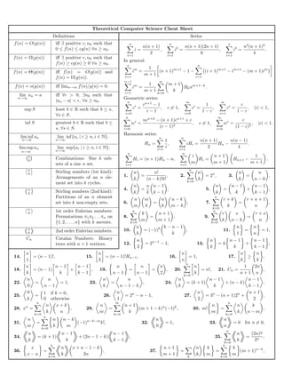
- 1. Theoretical Computer Science Cheat Sheet Definitions Series f (n) = O(g(n)) iff ∃ positive c, n0 such that n n n n(n + 1) n(n + 1)(2n + 1) n2 (n + 1)2 0 ≤ f (n) ≤ cg(n) ∀n ≥ n0 . i= , i2 = , i3 = . i=1 2 i=1 6 i=1 4 f (n) = Ω(g(n)) iff ∃ positive c, n0 such that In general: f (n) ≥ cg(n) ≥ 0 ∀n ≥ n0 . n n 1 f (n) = Θ(g(n)) iff f (n) = O(g(n)) and im = (n + 1)m+1 − 1 − (i + 1)m+1 − im+1 − (m + 1)im i=1 m+1 i=1 f (n) = Ω(g(n)). n−1 m 1 m+1 f (n) = o(g(n)) iff limn→∞ f (n)/g(n) = 0. im = Bk nm+1−k . i=1 m+1 k k=0 lim an = a iff ∀ > 0, ∃n0 such that n→∞ Geometric series: |an − a| < , ∀n ≥ n0 . n ∞ ∞ cn+1 − 1 1 c sup S least b ∈ R such that b ≥ s, ci = , c = 1, ci = , ci = , |c| < 1, c−1 1−c 1−c ∀s ∈ S. i=0 i=0 i=1 n ∞ ncn+2 − (n + 1)cn+1 + c c inf S greatest b ∈ R such that b ≤ ici = , c = 1, ici = , |c| < 1. s, ∀s ∈ S. i=0 (c − 1)2 i=0 (1 − c)2 Harmonic series: lim inf an lim inf{ai | i ≥ n, i ∈ N}. n n n→∞ n→∞ 1 n(n + 1) n(n − 1) Hn = , iHi = Hn − . lim sup an lim sup{ai | i ≥ n, i ∈ N}. i=1 i i=1 2 4 n→∞ n→∞ n n n i n+1 1 k Combinations: Size k sub- Hi = (n + 1)Hn − n, Hi = Hn+1 − . sets of a size n set. i=1 i=1 m m+1 m+1 n n Stirling numbers (1st kind): n n! n n n k Arrangements of an n ele- 1. = , 2. = 2n , 3. = , k (n − k)!k! k k n−k k=0 ment set into k cycles. n n n−1 n n−1 n−1 n 4. = , 5. = + , k Stirling numbers (2nd kind): k k k−1 k k k−1 Partitions of an n element n m n n−k n r+k r+n+1 set into k non-empty sets. 6. = , 7. = , m k k m−k k n n k=0 1st order Eulerian numbers: n n k k n+1 r s r+s Permutations π1 π2 . . . πn on 8. = , 9. = , m m+1 k n−k n {1, 2, . . . , n} with k ascents. k=0 k=0 n k−n−1 n n n 2nd order Eulerian numbers. 10. = (−1) k , 11. = = 1, k k k 1 n Cn Catalan Numbers: Binary n n−1 n n−1 trees with n + 1 vertices. 12. = 2n−1 − 1, , 13. =k + 2 k−1 k k n n n n n 14. = (n − 1)!, 15. = (n − 1)!Hn−1 , 16. = 1, 17. ≥ , 1 2 n k k n n n−1 n−1 n n n n 1 2n 18. = (n − 1) + , 19. = = , 20. = n!, 21. Cn = , k k k−1 n−1 n−1 2 k n+1 n k=0 n n n n n n−1 n−1 22. = = 1, 23. = , 24. = (k + 1) + (n − k) , 0 n−1 k n−1−k k k k−1 0 1 if k = 0, n n n+1 25. = 26. = 2n − n − 1, 27. = 3n − (n + 1)2n + , k 0 otherwise 1 2 2 n m n n x+k n n+1 n n k 28. xn = , 29. = (m + 1 − k)n (−1)k , 30. m! = , k n m k m k n−m k=0 k=0 k=0 n n n n−k n n 31. = (−1)n−k−m k!, 32. = 1, 33. = 0 for n = 0, m k m 0 n k=0 n n n−1 n−1 n (2n)n 34. = (k + 1) + (2n − 1 − k) , 35. = , k k k−1 k 2n k=0 n n x n x+n−1−k n+1 n k k 36. = , 37. = = (m + 1)n−k , x−n k 2n m+1 k m m k=0 k k=0
- 2. Theoretical Computer Science Cheat Sheet Identities Cont. Trees n n n n+1 n k k n−k 1 k x n x+k Every tree with n 38. = = n = n! , 39. = , vertices has n − 1 m+1 k m m k! m x−n k 2n k k=0 k=0 k=0 edges. n n k+1 n n+1 k 40. = (−1)n−k , 41. = (−1)m−k , Kraft inequal- m k m+1 m k+1 m k k ity: If the depths m m m+n+1 n+k m+n+1 n+k of the leaves of 42. = k , 43. = k(n + k) , m k m k a binary tree are k=0 k=0 n n+1 k n n+1 k d1 , . . . , dn : 44. = (−1)m−k , 45. (n − m)! = (−1)m−k , for n ≥ m, n m k+1 m m k+1 m 2−di ≤ 1, k k n m−n m+n m+k n m−n m+n m+k i=1 46. = , 47. = , n−m m+k n+k k n−m m+k n+k k and equality holds k k n +m k n−k n n +m k n−k n only if every in- 48. = , 49. = . ternal node has 2 +m m k +m m k k k sons. Recurrences Master method: Generating functions: T (n) = aT (n/b) + f (n), a ≥ 1, b > 1 1 T (n) − 3T (n/2) = n 1. Multiply both sides of the equa- 3 T (n/2) − 3T (n/4) = n/2 tion by xi . If ∃ > 0 such that f (n) = O(nlogb a− ) . . . 2. Sum both sides over all i for then . . . . . . which the equation is valid. T (n) = Θ(nlogb a ). 3log2 n−1 T (2) − 3T (1) = 2 3. Choose a generating function ∞ If f (n) = Θ(nlogb a ) then G(x). Usually G(x) = i=0 xi gi . T (n) = Θ(nlogb a log2 n). Let m = log2 n. Summing the left side 3. Rewrite the equation in terms of we get T (n) − 3m T (1) = T (n) − 3m = the generating function G(x). If ∃ > 0 such that f (n) = Ω(nlogb a+ ), T (n) − nk where k = log2 3 ≈ 1.58496. 4. Solve for G(x). and ∃c < 1 such that af (n/b) ≤ cf (n) Summing the right side we get for large n, then m−1 m−1 5. The coefficient of xi in G(x) is gi . n i 3 i Example: T (n) = Θ(f (n)). 3 =n 2 . i=0 2i i=0 gi+1 = 2gi + 1, g0 = 0. Substitution (example): Consider the following recurrence Let c = 3 . Then we have 2 Multiply and sum: i Ti+1 = 22 · Ti2 , T1 = 2. m−1 c −1m gi+1 xi = 2gi xi + xi . i n c =n i≥0 i≥0 i≥0 c−1 Note that Ti is always a power of two. i=0 We choose G(x) = i≥0 xi gi . Rewrite Let ti = log2 Ti . Then we have = 2n(clog2 n − 1) in terms of G(x): ti+1 = 2i + 2ti , t1 = 1. = 2n(c(k−1) logc n − 1) G(x) − g0 = 2G(x) + xi . Let ui = ti /2i . Dividing both sides of = 2nk − 2n, x i≥0 the previous equation by 2i+1 we get ti+1 2i ti and so T (n) = 3n − 2n. Full history re- k Simplify: = i+1 + i . G(x) 1 2 i+1 2 2 currences can often be changed to limited = 2G(x) + . history ones (example): Consider x 1−x Substituting we find i−1 ui+1 = 1 + ui , 2 u1 = 1 , 2 Solve for G(x): Ti = 1 + Tj , T0 = 1. x G(x) = . which is simply ui = i/2. So we find j=0 (1 − x)(1 − 2x) i−1 that Ti has the closed form Ti = 2i2 . Note that i Expand this using partial fractions: Summing factors (example): Consider 2 1 the following recurrence Ti+1 = 1 + Tj . G(x) = x − 1 − 2x 1 − x T (n) = 3T (n/2) + n, T (1) = 1. j=0 Subtracting we find Rewrite so that all terms involving T i i−1 = x 2 2i xi − xi are on the left side Ti+1 − Ti = 1 + Tj − 1 − Tj i≥0 i≥0 T (n) − 3T (n/2) = n. j=0 j=0 = i+1 (2 − 1)x i+1 . Now expand the recurrence, and choose = Ti . i≥0 a factor which makes the left side “tele- scope” And so Ti+1 = 2Ti = 2i+1 . So gi = 2i − 1.
- 3. Theoretical Computer Science Cheat Sheet √ √ 1+ 5 ˆ 1− 5 π ≈ 3.14159, e ≈ 2.71828, γ ≈ 0.57721, φ= 2 ≈ 1.61803, φ= 2 ≈ −.61803 i 2i pi General Probability 1 2 2 Bernoulli Numbers (Bi = 0, odd i = 1): Continuous distributions: If 1 1 1 b 2 4 3 B0 = 1, B1 = B2 = −2, B4 = 6, − 30 , Pr[a < X < b] = p(x) dx, 1 1 5 3 8 5 B6 = 42 , B8 = − 30 , B10 = 66 . a 4 16 7 Change of base, quadratic formula: then p is the probability density function of √ X. If 5 32 11 loga x −b ± b2 − 4ac Pr[X < a] = P (a), logb x = , . 6 64 13 loga b 2a then P is the distribution function of X. If 7 128 17 Euler’s number e: P and p both exist then 1 1 11 8 256 19 e=1+ 2 + 24 + 120 + · · · + 6 a x n P (a) = p(x) dx. 9 512 23 lim 1 + = ex . −∞ n→∞ n Expectation: If X is discrete 10 1,024 29 1 n 1 n+1 1+ n <e< 1+ n . 11 2,048 31 E[g(X)] = g(x) Pr[X = x]. 1 n e 11e 1 x 12 4,096 37 1+ =e− + 2 −O . n 2n 24n n3 If X continuous then 13 8,192 41 ∞ ∞ Harmonic numbers: 14 16,384 43 E[g(X)] = g(x)p(x) dx = g(x) dP (x). 1, 3 , 11 , 25 , 137 , 49 , 363 , 761 , 7129 , . . . 2 6 12 60 20 140 280 2520 −∞ −∞ 15 32,768 47 Variance, standard deviation: 16 65,536 53 ln n < Hn < ln n + 1, VAR[X] = E[X 2 ] − E[X]2 , 17 131,072 59 1 σ = VAR[X]. Hn = ln n + γ + O . 18 262,144 61 n For events A and B: 19 524,288 67 Factorial, Stirling’s approximation: Pr[A ∨ B] = Pr[A] + Pr[B] − Pr[A ∧ B] 20 1,048,576 71 1, 2, 6, 24, 120, 720, 5040, 40320, 362880, ... Pr[A ∧ B] = Pr[A] · Pr[B], 21 2,097,152 73 iff A and B are independent. √ n 1 n 22 4,194,304 79 n! = 2πn 1+Θ . Pr[A ∧ B] e n Pr[A|B] = 23 8,388,608 83 Pr[B] Ackermann’s function and inverse: 24 16,777,216 89 For random variables X and Y : 2j i=1 25 33,554,432 97 a(i, j) = a(i − 1, 2) j=1 E[X · Y ] = E[X] · E[Y ], 26 67,108,864 101 a(i − 1, a(i, j − 1)) i, j ≥ 2 if X and Y are independent. 27 134,217,728 103 α(i) = min{j | a(j, j) ≥ i}. E[X + Y ] = E[X] + E[Y ], E[cX] = c E[X]. 28 268,435,456 107 Binomial distribution: n k n−k Bayes’ theorem: 29 536,870,912 109 Pr[X = k] = p q , q = 1 − p, k Pr[B|Ai ] Pr[Ai ] 30 1,073,741,824 113 Pr[Ai |B] = n . n j=1 Pr[Aj ] Pr[B|Aj ] 31 2,147,483,648 127 n k n−k E[X] = k p q = np. Inclusion-exclusion: 32 4,294,967,296 131 k n n k=1 Poisson distribution: Pr Xi = Pr[Xi ] + Pascal’s Triangle e−λ λk i=1 i=1 1 Pr[X = k] = , E[X] = λ. n k k! 11 Normal (Gaussian) distribution: (−1)k+1 Pr Xij . k=2 ii <···<ik j=1 121 1 2 2 p(x) = √ e−(x−µ) /2σ , E[X] = µ. Moment inequalities: 1331 2πσ 1 14641 The “coupon collector”: We are given a Pr |X| ≥ λ E[X] ≤ , random coupon each day, and there are n λ 1 5 10 10 5 1 1 different types of coupons. The distribu- Pr X − E[X] ≥ λ · σ ≤ . 1 6 15 20 15 6 1 tion of coupons is uniform. The expected λ2 1 7 21 35 35 21 7 1 Geometric distribution: number of days to pass before we to col- lect all n types is Pr[X = k] = pq k−1 , q = 1 − p, 1 8 28 56 70 56 28 8 1 ∞ 1 9 36 84 126 126 84 36 9 1 nHn . 1 E[X] = kpq k−1 = . p 1 10 45 120 210 252 210 120 45 10 1 k=1
- 4. Theoretical Computer Science Cheat Sheet Trigonometry Matrices More Trig. Multiplication: C n (0,1) C = A · B, ci,j = ai,k bk,j . a b b h (cos θ, sin θ) k=1 C θ Determinants: det A = 0 iff A is non-singular. A (-1,0) (1,0) A c B det A · B = det A · det B, Law of cosines: c a c2 = a2 +b2 −2ab cos C. n (0,-1) B det A = sign(π)ai,π(i) . π i=1 Area: Pythagorean theorem: C 2 = A2 + B 2 . 2 × 2 and 3 × 3 determinant: a b A = 1 hc, 2 Definitions: = ad − bc, = 1 ab sin C, c d 2 sin a = A/C, cos a = B/C, a b c c2 sin A sin B csc a = C/A, sec a = C/B, b c a c a b = . d e f =g −h +i 2 sin C sin a A cos a B e f d f d e Heron’s formula: tan a = = , cot a = = . g h i cos a B sin a A aei + bf g + cdh √ Area, radius of inscribed circle: = − ceg − f ha − ibd. A = s · sa · sb · sc , 1 AB Permanents: s = 1 (a + b + c), 2 AB, . 2 A+B+C n sa = s − a, Identities: perm A = ai,π(i) . π i=1 sb = s − b, 1 1 sin x = , cos x = , Hyperbolic Functions sc = s − c. csc x sec x 1 Definitions: More identities: tan x = , sin2 x + cos2 x = 1, cot x ex − e−x e +e x −x 1 − cos x sinh x = , cosh x = , sin x = , 1 + tan2 x = sec2 x, 1 + cot2 x = csc2 x, 2 −x 2 2 2 e −e x 1 tanh x = x , csch x = , 1 + cos x sin x = cos π 2 −x , sin x = sin(π − x), e + e−x sinh x cos x = 2 , 1 1 2 sech x = , coth x = . cos x = − cos(π − x), tan x = cot π 2 −x , cosh x tanh x 1 − cos x tan x = 2 , Identities: 1 + cos x cot x = − cot(π − x), csc x = cot x − cot x, 2 1 − cos x cosh2 x − sinh2 x = 1, tanh2 x + sech2 x = 1, = sin x , sin(x ± y) = sin x cos y ± cos x sin y, sin x coth2 x − csch2 x = 1, sinh(−x) = − sinh x, = , cos(x ± y) = cos x cos y sin x sin y, 1 + cos x cosh(−x) = cosh x, tanh(−x) = − tanh x, 1 + cos x tan x ± tan y cot x = , tan(x ± y) = , 2 1 − cos x 1 tan x tan y sinh(x + y) = sinh x cosh y + cosh x sinh y, 1 + cos x cot x cot y 1 = , cot(x ± y) = , cosh(x + y) = cosh x cosh y + sinh x sinh y, sin x cot x ± cot y sin x 2 tan x sinh 2x = 2 sinh x cosh x, = , sin 2x = 2 sin x cos x, sin 2x = 1 + tan2 x , 1 − cos x cosh 2x = cosh2 x + sinh2 x, eix − e−ix cos 2x = cos2 x − sin2 x, cos 2x = 2 cos2 x − 1, sin x = , 2i 1 − tan2 x cosh x + sinh x = ex , cosh x − sinh x = e−x , eix + e−ix cos 2x = 1 − 2 sin2 x, cos 2x = , 1 + tan2 x cos x = , (cosh x + sinh x)n = cosh nx + sinh nx, n ∈ Z, 2 2 tan x cot2 x − 1 eix − e−ix tan 2x = 2 , cot 2x = , 2 sinh2 x = cosh x − 1, 2 cosh2 x = cosh x + 1. tan x = −i ix , 1 − tan x 2 cot x 2 2 e + e−ix sin(x + y) sin(x − y) = sin2 x − sin2 y, e2ix − 1 θ sin θ cos θ tan θ . . . in mathematics = −i 2ix , e +1 cos(x + y) cos(x − y) = cos2 x − sin2 y. you don’t under- sinh ix 0 0 √ 1 √ 0 sin x = , π 1 3 3 stand things, you i Euler’s equation: 6 2 2 3 √ √ just get used to eix = cos x + i sin x, eiπ = −1. π 2 2 cos x = cosh ix, 4 2 2 1 them. v2.02 c 1994 by Steve Seiden π √ 3 1 √ – J. von Neumann tan x = tanh ix . 3 2 2 3 i sseiden@acm.org π 2 1 0 ∞ http://www.csc.lsu.edu/~seiden
- 5. Theoretical Computer Science Cheat Sheet Number Theory Graph Theory The Chinese remainder theorem: There ex- Definitions: Notation: ists a number C such that: Loop An edge connecting a ver- E(G) Edge set tex to itself. V (G) Vertex set C ≡ r1 mod m1 c(G) Number of components Directed Each edge has a direction. . . . . . . Simple Graph with no loops or G[S] Induced subgraph . . . multi-edges. deg(v) Degree of v C ≡ rn mod mn ∆(G) Maximum degree Walk A sequence v0 e1 v1 . . . e v . if mi and mj are relatively prime for i = j. Trail A walk with distinct edges. δ(G) Minimum degree Path A trail with distinct χ(G) Chromatic number Euler’s function: φ(x) is the number of vertices. χE (G) Edge chromatic number positive integers less than x relatively n Connected A graph where there exists Gc Complement graph prime to x. If i=1 pei is the prime fac- i a path between any two Kn Complete graph torization of x then n vertices. Kn1 ,n2 Complete bipartite graph φ(x) = pi i −1 (pi − 1). e Component A maximal connected r(k, ) Ramsey number i=1 subgraph. Geometry Euler’s theorem: If a and b are relatively Tree A connected acyclic graph. prime then Projective coordinates: triples Free tree A tree with no root. 1 ≡ aφ(b) mod b. (x, y, z), not all x, y and z zero. DAG Directed acyclic graph. Eulerian Graph with a trail visiting (x, y, z) = (cx, cy, cz) ∀c = 0. Fermat’s theorem: each edge exactly once. Cartesian Projective 1 ≡ ap−1 mod p. Hamiltonian Graph with a cycle visiting (x, y) (x, y, 1) The Euclidean algorithm: if a > b are in- each vertex exactly once. y = mx + b (m, −1, b) tegers then Cut A set of edges whose re- x=c (1, 0, −c) gcd(a, b) = gcd(a mod b, b). moval increases the num- Distance formula, Lp and L∞ n If i=1 pei is the prime factorization of x ber of components. metric: i then Cut-set A minimal cut. (x1 − x0 )2 + (y1 − y0 )2 , pi i +1 − 1 n e Cut edge A size 1 cut. 1/p S(x) = d= . k-Connected A graph connected with |x1 − x0 |p + |y1 − y0 |p , pi − 1 d|x i=1 the removal of any k − 1 lim |x1 − x0 |p + |y1 − y0 | p 1/p . Perfect Numbers: x is an even perfect num- vertices. p→∞ ber iff x = 2n−1 (2n −1) and 2n −1 is prime. k-Tough ∀S ⊆ V, S = ∅ we have Area of triangle (x0 , y0 ), (x1 , y1 ) Wilson’s theorem: n is a prime iff k · c(G − S) ≤ |S|. and (x2 , y2 ): (n − 1)! ≡ −1 mod n. k-Regular A graph where all vertices 1 x1 − x0 y1 − y0 2 abs x − x . have degree k. 2 0 y2 − y0 M¨bius o inversion: k-Factor A k-regular spanning 1 if i = 1. Angle formed by three points: subgraph. 0 if i is not square-free. µ(i) = Matching A set of edges, no two of (−1)r if i is the product of (x2 , y2 ) r distinct primes. which are adjacent. 2 Clique A set of vertices, all of If θ which are adjacent. G(a) = F (d), (0, 0) 1 (x1 , y1 ) Ind. set A set of vertices, none of d|a which are adjacent. (x1 , y1 ) · (x2 , y2 ) cos θ = . then Vertex cover A set of vertices which 1 2 a F (a) = µ(d)G . cover all edges. Line through two points (x0 , y0 ) d d|a Planar graph A graph which can be em- and (x1 , y1 ): Prime numbers: beded in the plane. x y 1 ln ln n Plane graph An embedding of a planar x0 y0 1 = 0. pn = n ln n + n ln ln n − n + n ln n graph. x1 y1 1 n Area of circle, volume of sphere: +O , deg(v) = 2m. ln n A = πr2 , V = 4 πr3 . v∈V 3 n n 2!n π(n) = + + If G is planar then n − m + f = 2, so ln n (ln n)2 (ln n)3 If I have seen farther than others, f ≤ 2n − 4, m ≤ 3n − 6. it is because I have stood on the n +O . Any planar graph has a vertex with de- shoulders of giants. (ln n)4 gree ≤ 5. – Issac Newton
- 6. Theoretical Computer Science Cheat Sheet π Calculus Wallis’ identity: Derivatives: 2 · 2 · 4 · 4 · 6 · 6··· π =2· d(cu) du d(u + v) du dv d(uv) dv du 1 · 3 · 3 · 5 · 5 · 7··· 1. =c , 2. = + , 3. =u +v , dx dx dx dx dx dx dx dx Brouncker’s continued fraction expansion: 12 d(un ) du d(u/v) v du − u dv d(ecu ) du π 4. = nun−1 , 5. = dx dx , 6. = cecu , 4 =1+ 32 dx dx dx v2 dx dx 2+ 52 2+ 2+ 72 d(cu ) du d(ln u) 1 du 2+··· 7. = (ln c)cu , 8. = , dx dx dx u dx Gregrory’s series: 1 1 1 1 4 =1− 3 + − − ··· π + d(sin u) du d(cos u) du 5 7 9 9. = cos u , 10. = − sin u , dx dx dx dx Newton’s series: d(tan u) du d(cot u) du 1 1 1·3 11. = sec2 u , 12. = csc2 u , dx dx dx dx 6 = 2 + 2 · 3 · 23 + 2 · 4 · 5 · 25 + · · · π d(sec u) du d(csc u) du Sharp’s series: 13. = tan u sec u , 14. = − cot u csc u , dx dx dx dx 1 1 1 1 d(arcsin u) 1 du d(arccos u) −1 du π = √ 1− 1 + 2 − 3 +··· 15. =√ , 16. =√ , 6 3 ·3 3 ·5 3 ·7 dx 1−u 2 dx dx 1 − u2 dx 3 Euler’s series: d(arctan u) 1 du d(arccot u) −1 du 17. = , 18. = , dx 1 + u2 dx dx 1 + u2 dx π2 1 1 1 1 1 6 = 12 + 22 + 32 + 42 + 52 + ··· d(arcsec u) 1 du d(arccsc u) −1 du π2 1 1 1 1 1 19. = √ , 20. = √ , u 1−u 2 dx u 1−u 2 dx 8 = 12 + 32 + 52 + 72 + 92 + ··· dx dx π2 1 1 1 1 1 d(sinh u) du d(cosh u) du 12 = 12 − 22 + 32 − 42 + 52 − ··· 21. = cosh u , 22. = sinh u , dx dx dx dx Partial Fractions d(tanh u) du d(coth u) du 23. = sech2 u , 24. = − csch2 u , Let N (x) and D(x) be polynomial func- dx dx dx dx tions of x. We can break down d(sech u) du d(csch u) du N (x)/D(x) using partial fraction expan- 25. = − sech u tanh u , 26. = − csch u coth u , dx dx dx dx sion. First, if the degree of N is greater than or equal to the degree of D, divide d(arcsinh u) 1 du d(arccosh u) 1 du 27. =√ , 28. =√ , dx 1+u 2 dx dx u 2 − 1 dx N by D, obtaining N (x) N (x) d(arctanh u) 1 du d(arccoth u) 1 du = Q(x) + , 29. = , 30. = 2 , D(x) D(x) dx 1 − u2 dx dx u − 1 dx where the degree of N is less than that of d(arcsech u) −1 du d(arccsch u) −1 du 31. = √ , 32. = √ . D. Second, factor D(x). Use the follow- dx u 1 − u2 dx dx |u| 1 + u2 dx ing rules: For a non-repeated factor: Integrals: N (x) A N (x) = + , (x − a)D(x) x−a D(x) 1. cu dx = c u dx, 2. (u + v) dx = u dx + v dx, where N (x) 1 1 A= . 3. xn dx = xn+1 , n = −1, 4. dx = ln x, 5. ex dx = ex , D(x) x=a n+1 x For a repeated factor: dx dv du 6. = arctan x, 7. u dx = uv − v dx, N (x) m−1 Ak N (x) 1 + x2 dx dx = + , (x − a)m D(x) (x − a)m−k D(x) 8. sin x dx = − cos x, 9. cos x dx = sin x, k=0 where 1 dk N (x) 10. tan x dx = − ln | cos x|, 11. cot x dx = ln | cos x|, Ak = . k! dxk D(x) x=a 12. sec x dx = ln | sec x + tan x|, 13. csc x dx = ln | csc x + cot x|, The reasonable man adapts himself to the world; the unreasonable persists in trying to adapt the world to himself. Therefore 14. arcsin x dx = arcsin x + a a a2 − x2 , a > 0, all progress depends on the unreasonable. – George Bernard Shaw
- 7. Theoretical Computer Science Cheat Sheet Calculus Cont. 15. arccos x dx = arccos x − a a a2 − x2 , a > 0, 16. arctan x dx = x arctan x − a a a 2 ln(a2 + x2 ), a > 0, 17. sin2 (ax)dx = 1 2a ax − sin(ax) cos(ax) , 18. cos2 (ax)dx = 1 2a ax + sin(ax) cos(ax) , 19. sec2 x dx = tan x, 20. csc2 x dx = − cot x, sinn−1 x cos x n − 1 cosn−1 x sin x n − 1 21. sinn x dx = − + sinn−2 x dx, 22. cosn x dx = + cosn−2 x dx, n n n n tann−1 x cotn−1 x 23. tann x dx = − tann−2 x dx, n = 1, 24. cotn x dx = − − cotn−2 x dx, n = 1, n−1 n−1 tan x secn−1 x n − 2 25. secn x dx = + secn−2 x dx, n = 1, n−1 n−1 cot x cscn−1 x n − 2 26. cscn x dx = − + cscn−2 x dx, n = 1, 27. sinh x dx = cosh x, 28. cosh x dx = sinh x, n−1 n−1 29. tanh x dx = ln | cosh x|, 30. coth x dx = ln | sinh x|, 31. sech x dx = arctan sinh x, 32. csch x dx = ln tanh x , 2 33. sinh2 x dx = 1 4 sinh(2x) − 1 x, 2 34. cosh2 x dx = 1 4 sinh(2x) + 1 x, 2 35. sech2 x dx = tanh x, 36. arcsinh x dx = x arcsinh x − a a x2 + a2 , a > 0, 37. arctanh x dx = x arctanh x + a a a 2 ln |a2 − x2 |, x x arccosh − x2 + a2 , if arccosh x > 0 and a > 0, a 38. x arccosh a dx = a x x arccosh + x2 + a2 , if arccosh x < 0 and a > 0, a a dx 39. √ = ln x + a2 + x2 , a > 0, a2 + x2 dx 1 a2 40. = a arctan x , a > 0, 41. a2 − x2 dx = x 2 a2 − x2 + 2 arcsin x , a > 0, a2 + x2 a a 3a4 42. (a2 − x2 )3/2 dx = x (5a2 − 2x2 ) a2 − x2 + 8 8 arcsin x , a a > 0, dx dx 1 a+x dx x 43. √ = arcsin x , a > 0, 44. = ln , 45. = √ , a2 − x2 a a2 −x 2 2a a−x (a2 −x2 )3/2 a2 a2 − x2 a2 dx 46. a2 ± x2 dx = x 2 a2 ± x2 ± 2 ln x + a2 ± x2 , 47. √ = ln x + x2 − a2 , a > 0, x2 − a2 dx 1 x √ 2(3bx − 2a)(a + bx)3/2 48. = ln , 49. x a + bx dx = , ax2 + bx a a + bx 15b2 √ √ √ a + bx √ 1 x 1 a + bx − a 50. dx = 2 a + bx + a √ dx, 51. √ dx = √ ln √ √ , a > 0, x x a + bx a + bx 2 a + bx + a √ √ a2 − x2 a + a2 − x2 52. dx = a2 − x2 − a ln , 53. x a2 − x2 dx = − 1 (a2 − x2 )3/2 , 3 x x √ 2 2 2 a4 dx 1 a+ a2 − x2 54. x a2 − x2 dx = x 8 (2x −a ) a2 − x2 + 8 arcsin x a, a > 0, 55. √ = − a ln , a2 − x2 x x dx x2 dx 2 56. √ = − a2 − x2 , 57. √ = − x a2 − x2 + a arcsin a, 2 2 x a > 0, a2 − x2 a2 − x2 √ √ √ a2 + x2 2 + x2 − a ln a + a2 + x2 x2 − a2 58. dx = a , 59. dx = x2 − a2 − a arccos |x| , a a > 0, x x x dx x 60. x x2 ± a2 dx = 1 (x2 ± a2 )3/2 , 3 61. √ = 1 ln √ , x x2 + a2 a a+ a2 + x2