Sienna 6 bst

Computer Science 385
Analysis of Algorithms
Siena College
Spring 2011

Topic Notes: Binary Search Trees

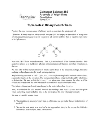
Possibly the most common usage of a binary tree is to store data for quick retrieval.
Definition: A binary tree is a binary search tree (BST) iff it is empty or if the value of every node
is both greater than or equal to every value in its left subtree and less than or equal to every value
in its right subtree.

6

4 9

2 5 7 10

1 3 8

Note that a BST is an ordered structure. That is, it maintains all of its elements in order. This
restriction allows us to build more efficient implementations of the most important operations on
the tree.
We will refer to the implementation of binary search trees in the structure package, the same
package we have been using for graph implementations.
Any interesting operation in a BST (get, add, remove) has to begin with a search for the correct
place in the tree to do the operation. Our implementation has a helper method used by all of these
to do just that. We want to find the BinaryTree whose root either contains the value, or, if the
value is not to be found, the node whose non-existent child would contain the value.
This is just a binary search, and is performed in the protected method locate.
Next, let’s consdier the add method. We will be creating a new BinaryTree with the given
value, and setting parent and child links in the tree to place this new value appropriately.
We need to consider several cases:

1. We are adding to an empty binary tree, in which case we just make the new node the root of
the BST.

2. We add the new value as a new leaf at the appropriate place in the tree as the child of a
current leaf. For example, add 5.5 to this tree:

CS 385 Analysis of Algorithms Spring 2011

6

4 9

2 5 7 10

1 3 8

to get

6

4 9

2 5 7 10

1 3 5.5 8

3. If the value is one that is already in the tree, the search may stop early, in which case we
need to add the new item as a child of the predecessor of the node found.
For example, adding 9 to the tree above:

6

4 9

2 5 7 10

1 3 5.5 8

9

We can choose to add duplicate values as either left or right children as long as we’re con-
sistent. Our implementation chooses to put them at the left.

Our add implementation used a helper method predecessor. We have this, plus a helper
method to ﬁnd the successor.
These are pretty straightforward. Our predecessor is the rightmost entry in our left subtree, and the
successor is the leftmost entry in the right subtree.
The get method is very simple. It’s just a locate, followed by a check to make sure the value
was found at the location.
remove is more interesting.
Again, there are a number of possibilities:

1. We are removing a leaf, which is very straightforward.

2


2. We are removing the root of the entire tree, in which case we need to change the root of the
BST.

3. We are removing an internal node, in which case we need to merge the children into a single
subtree to replace the removed internal node.

4. The item is not found, so the tree is unmodiﬁed and we return null.

The implementation separates out three important cases: removing the root, removing a node
which is a left subtree, or removing a node which is a right subtree. In each case, we replace the
removed node with a tree equivalent to its two subtrees, merged together. This is accomplished
through the removeTop method.
This method is also broken into a number of cases:

1. Easy cases: If either child of top is empty, just use the other child as the new top. Done.

2. Another easy case: top’s left child has no right child. Here, just assign top’s right to be the
right child of left child and call the left child the new top.

3. The more complex case remains: left child has a right child.
Here, we will proceed by locating the predecessor of the top node, make that the new top,
and rearrange the subtrees in the only way that retains the order of the entire tree.

What about complexity of these operations?
add, get, contains, and remove are all proportional to the height of the tree. So if the tree is
well-balanced, these are Θ(log n), but all are Θ(n) in the worst case.

Tree Sort
One of many ways we can use a BST is for sorting.
We can build a BST containing our data and then do an inorder traversal to retrieve them in sorted
order. Since the cost of entering an element into a (balanced) binary tree of size n is log n, the cost
of building the tree is
(log 1) + (log 2) + (log 3) + · · · + (log n) = Θ(n log n) compares.
The inorder traversal is Θ(n). The total cost is Θ(n log n) in both the best and average cases.
The worst case occurs if the input data is in order. In this case, we’re essentially doing an insertion
sort, creating a tree with one long branch. This results in a tree search as bad as Θ(n2 ).

Balanced Trees

3


Just having the same height on each child of the root is not enough to maintain a Θ(log n) height
for a binary tree.
We can deﬁne a balance condition, some set of rules about how the subtrees of a node can differ.
Maintaining a perfectly strict balance (minimum height for the given number of nodes) is often too
expensive. Maintaining too loose a balance can destroy the Θ(log n) behaviors that often motivate
the use of tree structures in the ﬁrst place.
For a strict balance, we could require that all levels except the lowest are full.
How could we achieve this? Let’s think about it by inserting the values 1,2,3,4,5,6,7 into a BST
and seeing how we could maintain strict balance.
First, insert 1:

1

Next, insert 2:

1

2

We’re OK there. But when we insert 3:

1

2

3

we have violated our strict balance condition. Only one tree with these three values satisies the
condition:

4


2
/
1 3

We will see how to “rotate” the tree to achieve this shortly.
Now, add 4:

2
/
1 3

4

Then add 5:

2
/
1 3

4

5

Again, we need to ﬁx the balance condition. Here, we can apply one of these rotations on the right
subtree of the root:

2
/
1 4
/
3 5

Now, add 6:

2
/
1 4
/
3 5

6

5


It’s not completely obvious how to fix this one up, and we won’t worry about it just now. We do
know that after we insert the 7, there’s only one permissible tree:

4
/
2 6
/ /
1 3 5 7

So maintaining strict balance can be very expensive. The tree adjustments can be more expensive
than the benefits.
There are several options to deal with potentially unbalanced trees without requiring a perfect
balance.

1. Red-black trees – nodes are colored red or black, and place restrictons on when red nodes
and black nodes can cluster.

2. AVL Trees - Adelson-Velskii and Landis developed these in 1962. We will look at these.

3. Splay trees – every reference to a node causes that node to be relocated to the root of the tree.
This is very unusual! We have a contains() operation that actually modifies the structure.
This works very well in cases where the same value or a small group of values are likely to
be accessed repeatedly.
We may talk more later about splay trees as well.

AVL Trees
We consider AVL Trees, developed by and named for Adelson-Velskii and Landis, who invented
them in 1962.
Balance condition: the heights of the left and right subtrees of any node can differ by at most 1.
To see that this is less strict than perfect balance, let’s consider two trees:

5
/
2 8
/ /
1 4 7
/
3

6


This one satisﬁes the AVL condition (to decide this, we check the heights at each node), but is not
perfectly balanced since we could store these 7 values in a tree of height 2.
But...

7
/
2 8
/
1 4
/
3 5

This one does not satisfy the AVL condition – the root node violates it!
So the goal is to maintain the AVL balance condition each time there is an insertion (we will ignore
deletions, but similar techniques apply).
When inserting into the tree, a node in the tree can become a violator of the AVL condition. Four
cases can arise which characterize how the condition came to be violated. Let’s call the violating
node A.

1. Insertion into the left subtree of the left child of A.
2. Insertion into the right subtree of the left child of A.
3. Insertion into the left subtree of the right child of A.
4. Insertion into the right subtree of the right child of A.

In reality, however, there are only two really different cases, since cases 1 and 4 and cases 2 and 3
are mirror images of each other and similar techniques apply.
First, we consider a violation of case 1.
We start with a tree that satisﬁes AVL:

k2

k1

Z
level n−1
X Y
level n

7


After an insert, the subtree X increases in height by 1:

k2

k1

Z
level n−1
Y
X level n
level n+1

So now node k2 violates the balance condition.
We want to perform a single rotation to obtain an equivalent tree that satisﬁes AVL.
Essentially, we want to switch the roles of k1 and k2 , resulting in this tree:

k1

k2

X Y Z
level n

For this insertion type (left subtree of a left child – case 1), this rotation has restored balance.
We can think of this like you have a handle for the subtree at the root and gravity determines the
tree.
If we switch the handle from k2 to k1 and let things fall where they want (in fact, must), we have
rebalanced.
Consider insertion of 3,2,1,4,5,6,7 into an originally empty tree.
Insert 3:

3

8


Insert 2:

3
/
2

Insert 1:

3 2
/ /
2 ---> 1 3
/
1

Here, we had to do a rotation. We essentially replaced the root of the violating subtree with the
root of the taller of its children.
Now, we insert 4:

2
/
1 3

4

Then insert 5:

2
/
1 3 <-- AVL violated here (case 4)

4

5

and we have to rotate at 3:

2
/
1 4
/
3 5

9


Now insert 6:

2 <-- AVL violated here (case 4)
/
1 4
/
3 5

6

Here, our rotation moves 4 to the root and everything else falls into place:

4
/
2 5
/
1 3 6

Finally, we insert 7:

4
/
2 5 <-- AVL violated here (case 4 again)
/
1 3 6

7

4
/
2 6
/ /
1 3 5 7

We achieve perfect balance in this case, but this is not guaranteed in general.
This example demonstrates the application of cases 1 and 4, but not cases 2 and 3.
Here’s case 2:
We start again with the good tree:

10


k2

k1

Z
level n−1
X Y
level n

But now, our inserted item ends up in subtree Y :

k2

k1

Z
level n−1
level n X
Y
level n+1

We can attempt a single rotation:

k1

k2

X
level n−1 Z
Y level n
level n+1

This didn’t get us anywhere. We need to be able to break up Y .
We know subtree Y is not empty, so let’s draw our tree as follows:

11


k3

k1

k2
D
A level n−1
level n B C
level n+1

Here, only one of B or C is at level n + 1, since it was a single insert below k2 that resulted in the
AVL condition being violated at k3 with respect to its shorter child D.
We are guaranteed to correct it by moving D down a level and both B and C up a level:

k2

k1 k3

A B C D
level n

We’re essentially rearranging k1 , k2 , and k3 to have k2 at the root, and dropping in the subtrees in
the only locations where they can ﬁt.
In reality, only one of B and C is at level n – the other only descends to level n − 1.
Case 3 is the mirror image of this.
To see examples of this, let’s pick up the previous example, which had constructed a perfectly-
balanced tree of the values 1–7.

4
/
2 6
/ /
1 3 5 7

At this point, we insert a 16, then a 15 to get:

12


4
/
2 6
/ /
1 3 5 7

16
/
15

Node 7 violates AVL and this happened because of an insert into the left subtree of its right child.
Case 3.
So we let k1 be 7, k2 be 15, and k3 be 16 and rearrange them to have k2 at the root of the subtree,
with children k1 and k3 . Here, the subtrees A, B, C, and D are all empty.
We get:

4
/
2 6
/ /
1 3 5 15
/
7 16

Now insert 14.

4
/
2 6
/ /
1 3 5 15
/
7 16

14

This violates AVL at node 6 (one child of height 0, one of height 2).
This is again an instance of case 3: insertion into the left subtree of the right child of the violating
node.
So we let k1 be 6, k2 be 7, and k3 be 15 and rearrange them again. This time, subtrees A is the 5,
B is empty, C is the 14, and D is the 16.

13


The double rotation requires that 7 become the root of that subtree, the 6 and the 15 its children,
and the other subtrees fall into place:

4
/
2 7
/ /
1 3 6 15
/ /
5 14 16

Insert 13:

4
/
2 7
/ /
1 3 6 15
/ /
5 14 16
/
13

What do we have here? Looking up from the insert location, the ﬁrst element that violates the
balance condition is the root, which has a difference of two between its left and right child heights.
Since this is an insert into the right subtree of the right child, we’re dealing with case 4. This
requires just a single rotation, but one done all the way at the root. We get:

7
/
4 15
/ /
2 6 14 16
/ / /
1 3 5 13

Now adding 12:

7
/
4 15
/ /

14


2 6 14 16
/ / /
1 3 5 13
/
12

The violation this time is at 14, which is a simple single rotation (case 1):

7
/
4 15
/ /
2 6 13 16
/ / /
1 3 5 12 14

Inserting 11:

7
/
4 15
/ /
2 6 13 16
/ / /
1 3 5 12 14
/
11

Here, we have a violation at 15, case 1, so another single rotation there, promoting 13:

7
/
4 13
/ /
2 6 12 15
/ / / /
1 3 5 11 14 16

(Almost done)
Insert 10:

15


7
/
4 13
/ /
2 6 12 15
/ / / /
1 3 5 11 14 16
/
10

The violator here is 12, case 1:

7
/
4 13
/ /
2 6 11 15
/ / / /
1 3 5 10 12 14 16

Then we ﬁnally add 8 (no rotations needed) then 9:

7
/
4 13
/ /
2 6 11 15
/ / / /
1 3 5 10 12 14 16
/
8

9

Finally we see case 2 and do a double rotation with 8, 9, and 10 to get our ﬁnal tree:

7
/
4 13
/ /
2 6 11 15
/ / / /
1 3 5 9 12 14 16
/
8 10

16


This tree is not strictly balanced – we have a hole under 6’s right child, but it does satisfy AVL.
You can think about how we might implement an AVL tree, but we will not consider an actual
implementation. However, AVL insert operations make excellent exam questions, so keep that in
mind when preparing for the ﬁnal.
The whole point of considering AVL trees is to maintain a reasonable balance, and hopefully, a
tree height that looks like log n. We will not do a detailed analysis, but the height n of an AVL tree
is guaranteed to satisfy the inequality:

⌊log2 n⌋ ≤ h < 1.44.05 log2 (n + 2) − 1.3277.

We have log factors on both sides, leading to Θ(log n) worst case behavior of search and insert
operations.

17

Sienna 6 bst

Recomendados

Recomendados

Más contenido relacionado

Destacado

Destacado (6)

Similar a Sienna 6 bst

Similar a Sienna 6 bst (20)

Más de chidabdu

Más de chidabdu (19)

Último

Último (20)

Sienna 6 bst