veanlo

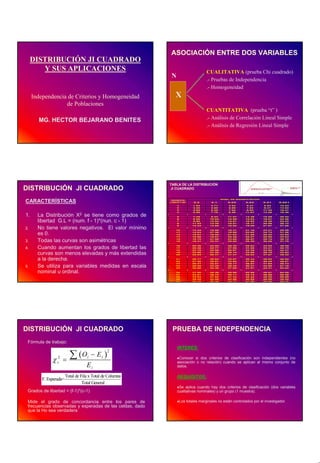
1. ASOCIACIÓN ENTRE DOS VARIABLES
DISTRIBUCIÓN JI CUADRADO
Y SUS APLICACIONES CUALITATIVA (prueba Chi cuadrado)
N
.- Pruebas de Independencia
.- Homogeneidad
Independencia de Criterios y Homogeneidad X
de Poblaciones
CUANTITATIVA (prueba “t” )
MG. HECTOR BEJARANO BENITES .- Análisis de Correlación Lineal Simple
.- Análisis de Regresión Lineal Simple
TABLA DE LA DISTRIBUCIÓN
DISTRIBUCIÓN JI CUADRADO JI CUADRADO
CARACTERÍSTICAS
NIVEL DE SIGNIFICACION
GRADOS
LIBERT AD 0.2 0.1 0.05 0.02 0.01 0.001
1 1.64 2.71 3.84 5.41 6.64 10.83
2 3.22 4.60 5.99 7.82 9.21 13.82
3 4.64 6.25 7.82 9.84 11.34 16.27
4 5.99 7.78 9.49 11.67 13.28 18.46
1. La Distribución X2 se tiene como grados de 5 7.29 9.24 11.07 13.39 15.09 20.52
libertad G.L = (num. f - 1)*(nun. c - 1)
6 8.55 10.64 12.59 15.03 16.81 22.46
7 9.80 12.02 14.07 16.62 18.48 24.32
8 11.03 13.26 15.51 18.17 20.09 26.12
No tiene valores negativos. El valor mínimo
9 12.24 14.68 16.92 19.08 21.67 27.88
2. 10 13.44 15.99 18.31 21.16 23.21 29.59
es 0. 11
12
13
14.63
15.81
16.98
27.28
18.55
19.81
19.68
21.03
22.36
22.62
21.05
25.47
24.72
26.22
25.69
31.26
32.94
34.53
3. Todas las curvas son asimétricas 14
15
18.15
19.31
21.06
22.31
23.68
25.00
26.87
28.26
29.14
30.58
36.12
37.70
Cuando aumentan los grados de libertad las
16 20.46 23.54 26.30 29.63 32.00 39.29
4. 17
18
20.46
22.76
24.77
25.99
27.59
28.87
31.00
32.35
33.41
34.80
40.75
42.31
curvas son menos elevadas y más extendidas 19
20
23.90
25.04
27.20
28.41
30.14
31.41
33.69
35.02
36.19
37.57
43.82
45.32
a la derecha. 21
22
26.17
27.30
29.62
30.81
32.67
33.92
36.34
37.66
38.93
40.29
46.80
48.27
23 28.41 32.01 35.17 38.97 41.64 49.73
5. Se utiliza para variables medidas en escala 24
25
29.55
30.68
33.20
34.38
36.42
37.65
40.27
41.57
42.98
44.31
51.18
52.62
nominal u ordinal. 26
27
31.80
32.91
35.36
36.74
38.88
40.11
42.86
44.14
45.61
46.96
54.05
55.48
28 34.03 37.92 41.34 45.42 48.28 58.89
29 36.25 32.09 42.56 46.69 49.59 38.20
30 36.25 40.26 43.77 47.96 50.89 59.70
DISTRIBUCIÓN JI CUADRADO PRUEBA DE INDEPENDENCIA
Fórmula de trabajo:
INTERES:
∑ ( Oi − E i )
2
χ c2 = Conocer si dos criterios de clasificación son independientes (no
asociación o no relación) cuando se aplican al mismo conjunto de
Ei datos.
Total de Fila x Total de Columna REQUISITOS:
F. Esperada=
Total General
Se aplica cuando hay dos criterios de clasificación (dos variables
Grados de libertad = (f-1)*(c-1) cualitativas nominales) y un grupo (1 muestra).
Mide el grado de concordancia entre los pares de Los totales marginales no están controlados por el investigador.
frecuencias observadas y esperadas de las celdas, dado
que la Ho sea verdadera
1

2. PRUEBA DE INDEPENDENCIA PRUEBA DE INDEPENDENCIA
Ejemplo: PROCEDIMIENTO
Evaluar si el toser por la mañana está asociado al fumar 1. Variables cualitativas, medidas en escala
cigarrillos en personas de 25 a 50 años de edad. nominal.
2. Planteamiento de Hipótesis.
¿Tose por la ¿Fuma Cigarrillos? Total Ho: Toser por la mañana es independiente de
Mañana? fumar cigarrillos
SI NO H1: Toser por la Mañana esta asociada a fumar
cigarrillos.
Si 45 24 69 3. Nivel de significación:
No 15 16 31
Para un nivel de significación de: α =0.05
Total 60 40 100
Cálculo de las frecuencias esperadas:
PRUEBA DE INDEPENDENCIA ¿Tose por la Mañana? ¿Fuma Cigarrillos? Total
SI NO
4. Estadístico de Prueba: Si 45 24 69
∑ (Oi − E i )
2 No 15 16 31
χ c2 = Total 60 40 100
Ei Su respectiva significancía es: P
69 x60
E 11 = = 4 1 .4
5. Criterios de Decisión: 100
69 x40
E 12 = = 2 7 .6
Ho se rechazaría si P≤α 100
31x60
E 21 = = 1 8 .6
100
6. Conclusión:
31x40
Se indica lo que se decidió con respecto a la hipótesis nula. E 22 = = 1 2 .4
100
(4 5 ) (1 5 ) (2 4 ) (1 6 )
2 2 2 2
− 4 1 .4 − 1 8 .6 − 2 7 .6 − 1 2 .4
χ 2
c = + + +
4 1 .4 1 8 .6 2 7 .6 1 2 .4
χ 2
c = 2 .5 3
PRUEBA DE HOMOGENEIDAD
DECISIÓN:
INTERES:
Como P ≥ 0.05 ( 0.1 < P < 0.2)
no se rechaza la Ho Conocer si dos o mas muestras provienen de poblaciones
Homogéneas con respecto a algún criterio de clasificación.
REQUISITOS:
CONCLUSIÓN:
Hay una variable y más de dos grupos independientes
El toser por la mañana es independiente del fumar
cigarrillos. Se usa cuando se hacen Estudios de Tipo Experimental
La Hipótesis Nula establece que las muestras se extraen de la
misma población
2

3. PRUEBA DE HOMOGENEIDAD PRUEBA DE HOMOGENEIDAD
PROCEDIMIENTO
Ejemplo:
1. Variables cualitativas, medidas en escala nominal.
Evaluar la efectividad de un antibiótico en tres
enfermedades de transmisión sexual.
2. Planteamiento de Hipótesis.
Curabilidad de ETS Ho: Las muestras provienen de poblaciones
la Enfermedad Total homogéneas según la curabilidad de pacientes con
A B C ETS.
H1: Las muestras no provienen de poblaciones
Si 75 25 70 170 homogéneas según la curabilidad de pacientes con
ETS.
No 15 45 10 70
Total 90 70 80 240 3. Nivel de significación
Para un nivel de significación de: α =0.05
PRUEBA DE HOMOGENEIDAD Cálculo de las frecuencias esperadas:
Estadístico de Prueba: 170x90 170x70
E11 = = 63.75 E12 = = 49.58
∑(O − E )
2
240 240
χc2 = i i
Su respectiva
170x80 70x90
Ei significancía es: P E13 = = 56.67 E21 = = 26.25
240 240
70x70 70x80
Criterios de Decisión: E22 = = 20.42 E23 = = 23.34
Ho se rechazaría si P ≤ α 240 240
( 75 − 63.75) ( 25 − 49.58) (10 − 23.34)
2 2 2
Conclusión:
Se indica lo que se decidió con respecto a la χc2 = + + ... +
63.75 49.58 23.34
hipótesis nula.
χc2 = 59.34
PRUEBA DE
HOMOGENEIDAD
DECISIÓN: χ c2 ≥ χ t2
Ho se rechaza 59.34 ≥ 5.99
CONCLUSIÓN:
Las muestras no provienen de poblaciones
homogéneas según la curabilidad de pacientes
con ETS.
3