Industry

© R.E.Marks 1998 Industry 1
© R.E.Marks 1998 Industry 2

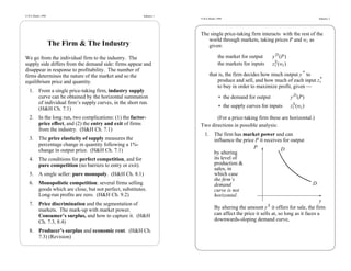
The single price-taking firm interacts with the rest of the
world through markets, taking prices P and wi as
The Firm & The Industry given:

We go from the individual firm to the industry. The the market for output y D (P)
supply side differs from the demand side: firms appear and the markets for inputs z S (wi )
i
disappear in response to profitability. The number of
firms determines the nature of the market and so the that is, the firm decides how much output y * to
equilibrium price and quantity. produce and sell, and how much of each input z *
i
to buy in order to maximize profit, given —
1. From a single price-taking firm, industry supply
curve can be obtained by the horizontal summation • the demand for output y D (P)
of individual firm’s supply curves, in the short run.
• the supply curves for inputs z S (wi )
i
(H&H Ch. 7.1)
2. In the long run, two complications: (1) the factor- (For a price-taking firm these are horizontal.)
price effect, and (2) the entry and exit of firms Two directions in possible analysis:
from the industry. (H&H Ch. 7.1)
1. The firm has market power and can
3. The price elasticity of supply measures the influence the price P it receives for output
percentage change in quantity following a 1%-
P .. D
change in output price. (H&H Ch. 7.1) by altering ...
its level of ...
4. The conditions for perfect competition, and for ...
production & ....
pure competition (no barriers to entry or exit). ....
sales, in .....
......
5. A single seller: pure monopoly. (H&H Ch. 8.1) which case .......
.........
the ﬁrm’s .....
6. Monopolistic competition: several firms selling demand D
goods which are close, but not perfect, substitutes. curve is not
Long-run profits are zero. (H&H Ch. 9.2) horizontal.
y
7. Price discrimination and the segmentation of
markets. The mark-up with market power. By altering the amount y S it offers for sale, the firm
Consumer’s surplus, and how to capture it. (H&H can affect the price it sells at, so long as it faces a
Ch. 7.3, 8.4) downwards-sloping demand curve,

8. Producer’s surplus and economic rent. (H&H Ch.
7.3) (Revision)

© R.E.Marks 1998 Industry 3 © R.E.Marks 1998 Industry 4

∂P
____ 1. Supply and Short-Run Response
and < 0 is evidence of market power.
∂y D (H&H Ch. 7.1)
(downwards sloping
firm’s demand curve)
1. When P < PV (where PV ≡ min(AVC)),
When this happens, we say there is then y * = 0 because TR < VC, and profit < 0.
imperfect competition,
and speak of these (definitions) When P > PV ,
monopoly one seller, then TR > VC and short-run π > 0 and π maximum
monopsony one buyer, with y * : MC (y * ) = P.
oligopoly a few sellers. (so long as increasing MC)
(strategic behaviour)
(→ game theory!) 2. The price-taking ﬁrm’s supply curve is its MC curve
above breakeven (π = 0). The industry supply
We consider this below (next lectures). curve or market supply is obtained by
horizontally adding all supply curves of
2. We can aggregate across a large number of small individual firms:
(price-taking) firms to obtain the
P
• industry supply of output, and = ΣSi
at any price of output (P 1 ) — i
• industry demand for inputs (e.g. labour).
how much will firm 1 supply?
(We assume that each firm produces identical output how much will firm 2 supply?
goods.)
• •
We shall answer these questions: • • ?
Q: at marketing-clearing equilibrium (S = D): • •
output
• what is the price of output? P
• what are the prices of inputs? wi The summation is similar to the summation of
• what are the quantities of outputs & inputs individual consumer demand curves to obtain
traded? y, zi the market demand curves (see above)
and are these equilibria stable? That is, will prices and but not exactly: there are complications:
quantities adjust to a market-clearing equilibrium,
where supply = demand?


2. Two complications in deriving the market supply >> Include H&H Fig 7.1, 7.2, 7.3 <<
curve from the individual firms’ supply curves:
Long-run Responses:

1. the number of firms is not fixed in the long run, but
will adjust in response to profitability,
∴ the number is responsive to output price P and
profits

− if a firm sees an opportunity for increased profit
in a new market, it may enter,
− if a firm is suffering low or negative profits in a
market, it must eventually leave the market.
____________________________________
∴ As price P rises, firms enter, cet. par.,
_ as price P falls, firms leave, cet. par.
___________________________________

$/unit
The effect of an ... D 1
.. S 2
increase in supply ..
... .... .. S
... .
(due to more firms) ...
... .... ... .... ....
is to bid down the .... .... ...
... .
....... ...
price, and reduce the ........ ..........
.. ...
profit of the marginal ...... ...... ............
.. .........
..... ....... D
firm to zero, i.e. no
........
more incentive for
entry or exit.
Q
The marginal firm is the one with the highest
average costs of production but positive profit still.


2. (Second complication) The Factor-Price Effect.
As the price of output P rises (say, cars) this >> Include H&H Fig 7.4 <<
may well have an effect on other markets (for
example, labour or
other markets in which cars are
an input to production)

An increase in price of output P may thus
• result in increased costs of production for the
firms,
• & result in a shift upwards in their supply
curves.
∴ the effective industry supply curve tends to
be steeper (less elastic) than the aggregate of
firms’ supply curves.

In conclusion:
• the short-run supply curve of a competitive (or price-
taking) firm is identical to its MC curve (above min
AVC),
• the short-run supply curve of a competitive industry is
the horizontal sum of firms’ supply curves, adjusted
for the factor-price effect,
• in the long run, the number of firms will change as
marginal firms (in cost terms, LRAC = P, ∴π = 0)
enter or leave in response to positive or negative
profit opportunities.


3. Price Elasticity of Supply: 4. Pure Competition
A perfectly competitive market satisfies the following
Let κ denote the price elasticity of supply: three conditions:
∆Q S Q S 1. numerous buyers
_ _______ (arc) ⇒ price takers
industry κ ≡ numerous sellers
∆P P
∂Q
_ S __ (point)
____ P ∴ there is no market power for an individual buyer
≡ or seller to affect the market price.
∂P Q
for a firm, 2. A homogenous good & identical buyers
∂Q S P (or arm’s length deals)
κi = _ ___ ___
i
∴ no price discrimination.
(point)
∂P Qi
κi +ve 3. Perfect information of all offers to buy & sell
∴ → there is one equilibrium price: S (P) = D (P).
+ 4. An additional condition ⇒ pure competition:
Defn. The price elasticity of supply is the % change in there are no barriers to entry or exit
output offered in response to a 1% increase in price of ∴ zero long-run proﬁt at the margin.
output.
1, 2, 3 ⇒ • individual consumers face horizontal
supply curves
n
But for the industry, κ ≤ Σ si κ i , (note the inequality) • individual firms face horizontal
i =1 supply curves (inputs)
• individual firms face horizontal
QS
where si = _____ is the market share
i
_
_________________________________
demand curves (outputs)
Σ QS where _ price: market supply = market demand
i _________________________________
and κ i is the price elasticity of supply of firm i. ∴ price = marginal cost to producers
(The inequality is because of a time period for = marginal value for consumers
adjustment, and entry or exit of firms, and the
.
factor-price effect.) P .... ....... S = Σ MCi
..... .....
....... ......
.......... ..............
.
.....................................
.................... ...... D = Σ Dj

Q


<<Smith Figs 8-5, 8-6 >>
..
P ... .. S
... ..
... ..
... .. MCi
.... ... .. ACi
.
.... .... ...... .. ....
.....
... ......
....... .. ........
..... ............. ........... ... ...........
.... ........... D ....................
....... ..
.....
........
Q output yi
Industry Price-Taking Firm i
Short run:
P > SRAC ∴ profit is positive

Long-run equilibrium when:
P = LRMC = min LRAC
and profit is zero.

In the diagrams (Smith 8-5, 8-6):
quantity A 2 is less than A 1
competitive price PA 2 is less than PA 1 .

For the price-taking firm:
• MR ≡ P = MC,
• rising marginal costs MC, and
• non-negative profits π .
• For the marginal firm, profits are zero (π = 0).
Although the industry demand curve is downwards
sloping, the firm sees only a horizontal demand curve.


5. Pure Monopoly P For a competitive, price-taking (PT) firm, by definition,
.. D = AR = P = P (Q)
.. the demand curve is horizontal (|η P | = ∞)
..
The single seller (monopoly) .. D ≠ MR dP
..
.. ∴ ___ = 0
faces a downward-sloping ... dQ
...
demand curve—it possesses ... ∴ MR = P
..
..
market power, and can choose .. Hence π is max. at Q*: Price = Marginal Cost (Q*)
..
...
any combination (P,Q) on the ... For a firm with market power,
... dP
demand curve to maximize its ...
... the demand curve slopes down & ___ < 0
... dQ
profit π . But choose Q ...
...
to maximise profit π .
.... ∴ MR ≠ P
.
Q dP
MR (Q) = P × (1 + __ ___ )
Q __________________________________
P dQ
π = TR (Q) − TC (Q) _1
__
MR (Q) = AR × (1 + P )
_ η
_________________________________
dπ dTR dTC ≤ AR = P × Q Q = P
max π ⇒ ___ = 0 = ____ − _ ___ i.e. MR (Q)
Q dQ dQ dQ
P AR (Q) ... S . = MC (Q)
PT
∴ MR (Q * ) = MC (Q * ) for π max. Remember:
... .
... ..
→ Q *
→ P *
... η P ≤ 0 ..
.. ... ...
... ....
..
....
d(P × Q) Q * is the output: .... ....
Marginal Revenue MR ≡ ________ M
.... ....
dQ
MR (Q * ) = MC (Q * )
M ....
.... ...
_1
__ M
..... ...
= P × (1 + P ) ....... ...
η Not P PT and Q PT when
C C ...
.
≤ P, (i.e., market power).
Supply = Demand
because the price elasticity of demand η P is negative. Q
∴ P ≥ MC with market power Where is MR (Q)?


100 In the long run . . .
Price Demand = AR = P
¢ ( . . . we’re all dead − J.M. Keynes)
Competitive market:
80
$/unit
AR = P = MC = AC MC (y)
AC (y)
& π =0 .......
..
. .....
P1
........
......... . ........
60 because ...............................................
.
AR = AC P2 .. . AR = D
....
.....
.............
40
output/period
MC = AC = 30¢
..................................................................................................... so: for the marginal firm, proﬁt is zero, having been
competed away by new entrants.
20
Long-run equilibrium when:
MR P = LRMC = min LRAC
and economic profit is zero.
1 2 3 4 5 6 7 8 9 10
Quantity Q The positive profits attract new entrants, whose output
in aggregate reduces the price at which supply equals
demand, until profits disappear (at least at the margin).

TR = P × Q, P = P (Q) To attain a competitive advantage, firms want to
secure a market position that protects from imitation
∆ TR = P × ∆ Q + ∆ P × Q and entry.
∂ TR ∂
____ = _ P (Q) Q + P
MR ≡ _ ______
∂Q ∂Q
Q: At what quantity is Revenue maximised?


6. Monopolistic Competition: Summary:
1. Prices of substitutes affect the demand curve,
For a firm (a monopoly ?) with market power (i.e. facing
downwards-sloping. (imperfect substitutes)
a downwards-sloping demand curve) with other firms
selling close substitutes, there is competition as firms
2. Assume that each firm takes others’ actions constant
change the prices of the close substitutes, which results in
& then sets sales (Q * ) so that
SR
a shift to the left in the demand curve that our firm faces.
MR(Q * ) = MC(Q * ) (SR ⇒ Short Run)
SR SR
→ Monopolistic Competition to maximize its profit (Q * → P * ).
SR
...
D′ .... D ..
..
....
..... .. 3. In general, P * > AC (Q * ) for each firm, so that
...... .. AC profit π is positive in the short run.
$/unit .. . ....... ...
.. .... ........ ... ⇒ attractive for new firms to produce close
... ....
... ...... ............. ......
.......................
......... . . ........................ substitutes in the long run.
..
...........
......................... ...... D
...........
........ D′ 4. In the medium-to-long run, new entrants invest, and
the original firms’ demand curves move to the left,
as their market share falls.
output/period 5. In the long run (LR), all profits will be bidded away
Conditions for Monopolistic Competition: for the marginal firm, with
AR = D ≡ P = AC ∴ π =0
1. firms compete by selling differentiated (such as
branded) products; substitutes but not perfect and maximum profit point on demand curve
substitutes; so they have some market power; (i.e. output Q * : MR (Q * ) = MC (Q * ))
LR LR LR

2. free entry and exit; no barriers; ∴ the demand curve must be tangent to the AC curve at
3. firms do not behave strategically, they assume their the price & output chosen. (LR: long run)
competitors’ actions fixed;
(See the T-shirt case.)
4. buyers are price takers; no bargaining.


.
.. ..
..
.. ..
D′ .. D .. D′ .. D
.. .. ..
.. .. . ..
. .. .. . ..
.
... .. . ..
...
.
...
... .. AC . ... AC
$/unit ... .. $/unit . ... MC = S
. .. .... .. .
.. ..
. ...
. .. .... .. ...
...
.
.. ..
.. .. .... .. .. ... .. ..
.. ...
..... .. .. .... .. ..
......
........ .. .. .. ..... .. ..
.. .... ........... ... .. ..... .. ..
.. ... .. ... ... .. .......
.. ... ..
.. ... ... ............................. ... ...
.. ...............................
.
...... ... ... ...
... ... ... .. D = AR
........
....................... ... D ....
.... ....
.....
.... ..
. .....
..... ....... .................
...... ....................... ........
...... .. .......
D′ ..
.. D′ = AR′
..
..
..
..
..
..
..
....
.........
output/period
Monopolistic Competition

Long-run equilibrium at the margin. output/period
(Remember: Competitive Pricing
average profit = average revenue – average cost.) and
There will be excess capacity: Monopoly Pricing
firms will not operate at minimum AC, and so they could
reduce AC by increasing output.
Why don’t they?


Assume: Many Buyers
________________________________________
_ Number of Sellers
_______________________________________
_ One A Few Many
_____________________________________________________
HOMOGENEOUS
Homogenous Pure Homogeneous Pure or
_ Product Monopoly Oligopoly Competition
_____________________________________________________ DIFFERENTIATED?
Differentiated Pure Differentiated Monopolistic
_ Product Monopoly Oligopoly Competition
_____________________________________________________ Degree of Substitutability?

Market Structure • Physical Attributes
• Ancillary Services
(One buyer, many sellers: monopsony.)
• Geographical Location
• Subjective Image
“I think it’s wrong only one company
makes the game Monopoly”
— US humorist, Steve Wright


Same seller, but ...
7. Price Discrimination

When a company which possesses some market power
charges its consumers different prices for essentially the
same product.
With market-power, the profit-maximization output y * is
Unequal markups: given by:
MR (y * ) = MC (y * )
P1 P2
_____ ≠ _____ > 1
MC 1 MC 2 but since (with uniform pricing):
P = D = AR > MR
⇒ PRICE DISCRIMINATION! it is not the case that P = MC .
across customers 1, 2 Instead,
P > MC
Perhaps because of: _ MC
________ (see above)
P =
_1
____
Different Customers (e.g. young, old, sex) 1−
|ηP |
• Different Time _P
___ _ 1
________ > 100%
∴ =
MC _1
____
• Different Place 1−
|ηP |
• Different Appearance when elastic: |η P | >1
= the mark-up (or P /MC–1).
(Note:
_ P > 1 implies market power. Why?)
___
The monopolist would like to segment the market
MC according to the price elasticity of demand η P and charge
higher prices for those consumers with lower elasticities of
demand.
Similarly: Taxes: on items with lower η ? Which?

© R.E.Marks 1998 Revision Industry 25 © R.E.Marks 1998 Revision Industry 26

Price Discrimination can take three broad forms: Total output must be such that marginal cost
equals marginal revenue across all groups
1. First-Degree Price Discrimination
(otherwise the firms are not maximising profits).
To capture all the consumers’ surplus, the firm with Total output is determined by horizontally summing
market power would like to charge each of its the marginal revenues of all groups and equating
customers the maximum price that customer is this sum with the marginal cost of total production.
willing to pay for each unit sold. Perfect price
discrimination. Remember that the mark-up formula gives:
2. Second-Degree Price Discrimination 1
__ ), η < 0
MR = P (1 +
In some markets (water, electricity, etc.) each η
consumer buys many units of the good over any and MR 1 = MR 2 implies that the ratio of prices in
given period, and the consumer’s demand falls with two segments is
the number of units bought.
In this situation, a firm can discriminate P1 (1 + 1/η 2 )
___ = _________
according to quantity bought. Multi-part pricing or P2 (1 + 1/η 1 )
declining block pricing, where the price for later
blocks bought is lower than the price for the earlier so the higher price is charged to the consumers with
blocks. the lower demand elasticity, as expected.

3. Third-Degree Price Discrimination 4. The Two-Part Tariff
The firm segments the market into two or more Another way of extracting consumer surplus:
groups with separate demand curves for each group, • charge an up-front fee T (for membership or
and charges the members of each group the same entrance or connection or a “monthly service
price, but members of different groups different fee”) and then
prices.
• charge a further per-unit price P for usage (for
This is the most common version of price
discrimination (haircuts, airfares, generic brands, use or rides or phone calls or water litres).
student and pensioner discounts). How to set the connect/entry fee T and the usage fee
For the groups, total output must be divided P? For a single consumer: let P = MC and T equal
between groups to equalise their marginal revenues the entire consumer surplus.
(otherwise firms are not maximising profits).

© R.E.Marks 1998 Revision Industry 27 © R.E.Marks 1998 Revision Industry 28

8. Consumers’ Surplus P S = MC ..
P D .. 8.1 Producers’ Surplus ..
... and Economic Rent ..
Remember: each point on ... ..
.. ..
the demand curve gives the C.S. ....... ..
..... ...
highest uniform price at ...... Each point on the supply ...
....... ....
which consumers are P 1 ........ curve (the MC curve for D .... D
........ D price-taking firms) P1 ....
willing to buy the P.S. ......
gives the lowest uniform .....
corresponding quantity of ......
.......
output. price which suppliers are ..................
Q1 Q willing to sell the
corresponding quantity of
At price P 1 there exist some consumers (represented by output.
the demand curve to the left) whose net willingness to pay Q1 Q
is still positive. The firm’s view: P.S. = TR − VC
∴ π = P.S. – FC
At price P 1 they gain consumers’ surplus, which (if their At price P 1 there exist some producers (represented by the
expenditure is a small fraction of their total expenditure, so supply curve to the left) who would sell at prices below
that there are no income effects with the price change) P 1 : their net willingness to sell at P 1 is still positive.
equals the area above the price and below the demand At price P 1 they gain producers’ surplus, or economic
curve. rent: a return to producers over and above the minimum
necessary to induce them to supply Q 1 in aggregate. P.S.
So consumers’ surplus is a willingness to pay over and equals the area below the (uniform) price and above the
above the uniform price (at uniform pricing or general supply (MC) curve.
pricing).
P S
A monopolist might like to segment the market and price
discriminate to increase his or her producers’ surplus at P1 D
the expense of consumers’ surplus.
rent

Q1 Q


________________________________________________________________

In the long run, monopolistic-competition equilibrium (1) (2)
(3) (4) (5) (6)
Consumer’s Total Marginal Profit
there will be excess capacity, Quantity Total Revenue Revenue with
Price Demanded Willingness(with perfect (with perfect AC =MC =0.3
i.e. firms will not operate at the minimum efﬁcient To Pay price disc.) price disc.) π = TR − TC
scale (y′, which results in the minimum AC), and so (1) × (2) ∆ (4) (4)–[(2)×0.30]
they could reduce AC by increasing output. ________________________________________________________________

P $1.00 1 $1.00 $1.00 $0.70
0.90 2 1.90 1.90 0.90 1.30
..... 0.80 3 2.70 2.70 0.80 1.80
.....
..... 0.70 4 3.40 3.40 0.70 2.20
.....
..... ... S
.....
..... ..... 0.60 5 4.00 4.00 0.60 2.50
..... ... 0.50 6 4.50 4.50 0.50 2.70
..... ....
..... .... 0.40 7 4.90 4.90 0.40 2.80
.....
..... ....
C.S. .......... .... 0.30 8 5.20 5.20 0.30 2.80
. ..... 0.20 9 5.40 5.40 0.20 2.70
..... .....
.....
..... ..... ..... 0.10 10 5.50 5.50 0.10 2.50
......... ________________________________________________________________
... ...... ..........
P.S. ...... .....
.. .......
.....
.....
.....
......... ..... MC = AC ⇒ constant cost firm
.......... .....
.................
.................... .....
.....
.....
.....
..... D

Q


100 9. Summary
Price Demand = AR = P
¢
In this section, we have considered:
80 1. How industry supply curves are derived from those
of individual firms, and the complications of
achieving this, in the short run and the long.
60 2. The differences between pure and perfect
competition, at one extreme, and
3. The use of market power by a proﬁt-maximising
40 monopolist, at the other extreme.
MC = AC = 30¢
..................................................................................................... 4. What the long-run equilibrium condition of zero
profits for the marginal ﬁrm means when firms face
20 horizontal demand curves (no market power) or
downwards-sloping demand curves (with market
MR power) in the case of monopolistic competition.
5. How and why firms with market power might
1 2 3 4 5 6 7 8 9 10 segment the market and price discriminate in order
Quantity to capture more of consumers’ surplus and so
increase their profits.
6. Three types of price discrimination: perfect price
TR = P × Q, P = P (Q)
discrimination, block price discrimination
∆ TR = P × ∆ Q + ∆ P × Q (declining), segmenting the market. Two-part tariff:
∂ TR ∂
____ = _ P (Q) Q + P a connect charge plus a usage charge.
MR ≡ _ ______
∂Q ∂Q 7. The meaning of economic rent, and the relationship
Monopoly PM = between producers’ surplus and profit.
MR (Q * ) = MC (Q * ), ∴ Q * =
M M M
πM =
Competitive PC =
Q* =
C
πC =

Industry

Recomendados

Recomendados

Más contenido relacionado

La actualidad más candente

La actualidad más candente (17)

Similar a Industry

Similar a Industry (20)

Último

Último (20)

Industry