Ku, E.M., Elliott, S.J. and Lineton, B. (2008). ‘Statistics of instabilities in a state space model of the cochlea,’ J. Acoust. Soc. Am., 124, (2), 1068-1079.

1. Statistics of instabilities in a state space model of the human
cochlea
Emery M. Ku,a Stephen J. Elliott, and Ben Lineton
Institute of Sound and Vibration Research, University of Southampton, Southampton,
United Kingdom SO17 1BJ
Received 16 January 2008; revised 8 May 2008; accepted 8 May 2008
A state space model of the human cochlea is used to test Zweig and Shera’s 1995 “The origin of
periodicity in the spectrum of evoked otoacoustic emissions,” J. Acoust. Soc. Am. 98 4 , 2018–
2047 multiple-reflection theory of spontaneous otoacoustic emission SOAE generation. The state
space formulation is especially well suited to this task as the unstable frequencies of an active model
can be rapidly and unambiguously determined. The cochlear model includes a human middle ear
boundary and matches human enhancement, tuning, and traveling wave characteristics. Linear
instabilities can arise across a wide bandwidth of frequencies in the model when the smooth spatial
variation of basilar membrane impedance is perturbed, though it is believed that only unstable
frequencies near the middle ear’s range of greatest transmissibility are detected as SOAEs in the ear
canal. The salient features of Zweig and Shera’s theory are observed in this active model given
several classes of perturbations in the distribution of feedback gain along the cochlea. Spatially
random gain variations are used to approximate what may exist in human cochleae. The statistics of
the unstable frequencies for random, spatially dense variations in gain are presented; the average
spacings of adjacent unstable frequencies agree with the preferred minimum distance observed in
human SOAE data. © 2008 Acoustical Society of America. DOI: 10.1121/1.2939133
PACS number s : 43.64.Kc, 43.64.Jb, 43.40.Vn, 43.64.Bt BLM Pages: 1068–1079
I. INTRODUCTION self-oscillation, when it is normally so close to instability .”
The existence of a cochlear amplifier CA was first pos- Evidence in the literature suggests that SOAEs are associated
tulated by Gold 1948 , who argued an electromechanical with BM oscillations. For example, Nuttall et al. 2004
action is necessary to counteract the heavy viscous damping measured a SOAE that had a counterpart in spontaneous me-
in the fluid-filled cochlea. The discovery of spontaneous chanical vibration of the BM at the same frequency. Further
otoacoustic emissions SOAEs by Kemp 1979 has long work performed by Martin and Hudspeth 2001 considered
served as indirect evidence supporting the presence of a CA. how locally unstable elements of the CA may be responsible
It is now widely accepted that the outer hair cells situated in for SOAEs. However, without careful tuning, a local-
the organ of Corti actively enhance the motion of the basilar oscillator model fails to account for the regular spacings be-
membrane BM e.g., Diependaal et al., 1987 , which gives tween unstable frequencies observed in mammalian SOAEs.
rise to a mammal’s sharply tuned sense of hearing. However, The strong peak in the distribution of spacings between
the precise mechanism underlying the generation of SOAEs adjacent SOAE frequencies, termed the preferred minimum
is still in debate. distance PMD , has been demonstrated by various studies
SOAEs are believed to be a feature of a normally func- Dallmayr, 1985, 1986; Talmadge et al., 1993; Braun, 1997 .
tioning CA, as they are commonly detected in an estimated A similar value is found in the average frequency spacings
range of 33%–70% of all normally hearing ears Talmadge between the spectral peaks of SFOAEs and TEOAEs when
et al., 1993 . Where SOAEs are detected, stimulus measured in the ear canal Zwicker and Schloth, 1984;
frequency-, distortion product- and transient evoked- Shera, 2003 . The PMD corresponds to a frequency spacing
otoacoustic emissions SFOAEs, DPOAEs, and TEOAEs of approximately 0.4 bark, or a distance of about 0.4 mm
are often present. There is evidence to suggest that all forms along the human cochlea Dallmayr, 1985, 1986 . Most
of OAEs are related and directly tied to the sensitivity of SOAEs occur in the range of 0.5– 6 kHz Probst et al., 1990
hearing Zwicker and Schloth, 1984; McFadden and Mishra, and demonstrate the PMD, though Zweig and Shera 1995
1993; Talmadge and Tubis, 1993; Shera and Guinan, 1999 . and Shera 2003 showed that the average spacings of both
Two primary classes of cochlea-based theories regarding the SOAEs and the spectral peaks of SFOAEs measured in the
production of SOAEs are discussed below: a local-oscillator ear canal vary somewhat with frequency.
model and a distributed backscattering concept. Strube 1989 argued that a periodic variation or “corru-
Gold 1948 first formed the basis of a local-oscillator gation” in the micromechanical parameters would also give
model of SOAE generation when he proposed that a pertur- rise to the observed PMD in SFOAE and TEOAE measure-
bation may “bring an active element into the region of ments in the ear canal. This was said to arise given distrib-
uted backscattering of the traveling wave TW similar to the
phenomenon of Bragg reflection in a crystal. In this theory,
a
Electronic mail: ek@isvr.soton.ac.uk. the period of the corrugation must correspond to one-half of
1068 J. Acoust. Soc. Am. 124 2 , August 2008 0001-4966/2008/124 2 /1068/12/$23.00 © 2008 Acoustical Society of America

2. the wavelength of the TW, thus generating constructive in- model of linear cochlear mechanics. Previous work has re-
terference at particular frequencies. Kemp 1979 also pro- lied upon phenomenological methods Zweig and Shera,
posed a theory of SOAE generation which assumed a distrib- 1995; Shera, 2003 , or multiple time-domain simulations
uted backscattering mechanism; his theory required multiple Talmadge et al., 1998 , to support this theory. In contrast, a
internal reflections of forward- and backward-traveling state space formulation of the cochlea Elliott et al., 2007 is
waves between the middle ear boundary and an inhomoge- used here that is capable of rapidly and unambiguously cal-
neous region of the cochlea. culating the unstable frequencies in a given linear model.
Since Kemp 1979 first presented the idea, numerous This method is thus especially well suited to generating the
authors have made contributions to the multiple-reflection large number of results from individual cochleae necessary
theory Zwicker and Peisl, 1990; Zweig, 1991; Shera and to ensure statistically significant data.
Zweig, 1993; Talmadge and Tubis, 1993; Zweig and Shera, Section II presents the revisions necessary to adapt the
1995; Allen et al., 1995; Talmadge et al., 1998; Shera and original model Neely and Kim, 1986 , on which the state
Guinan, 1999; Shera, 2003 . Shera and Zweig 1993 pro- space model of Elliott et al. 2007 was based, from repre-
posed that a spatially dense and random array of reflection senting a cat cochlea to representing a human cochlea. For
sites exists along the entire cochlea which acts in concert instance, a boundary approximating the human middle ear is
with the middle ear boundary to form standing waves, which now included. The features of the model that are pertinent to
Shera 2003 likens to a laser cavity. This concept was fully the “cochlear laser” theory, such as the wavelength of a TW
developed in Zweig and Shera 1995 . Though energy is re- at its peak as a function of position, are examined. Sample
flected at all frequencies by a perturbation along the cochlea, frequency responses and the stability of a base line cochlear
wavelets scattered from forward-traveling waves that peak in model are also briefly described.
the region of the inhomogeneity dominate the response, since In Sec. III, the smoothly varying BM impedance along
the amplitude is highest there. the cochlea is perturbed with a variety of spatial inhomoge-
For an active standing wave resonance to develop in this neities in the micromechanical feedback gain in order to in-
multiple-reflection theory, the spatial distribution of inhomo- troduce reflection sites. The following inhomogeneities are
geneities in the given region must contain components at the tested: a step change in gain; sinusoidal variations in gain;
wavenumber that creates constructive interference with the and band-limited spatially random variations in gain are ap-
incoming wave, just as with Bragg scattering Shera and plied in order to simulate what may exist in human cochleae.
Zweig, 1993; Zweig and Shera, 1995 . Further requirements A large number of simulations from the last category are
include an active region between the middle ear boundary performed. The spacings of adjacent unstable frequencies in
and the reflection site to overcome the viscous damping in the randomly perturbed cochlear models are collected and
the cochlea, and a TW frequency that undergoes an integer statistically analyzed at the end of this section.
number of cycles of round-trip phase change between the
middle ear and the cochlear reflection site; this naturally
gives rise to the PMD in SOAEs measured in the ear canal.
II. MODEL DESCRIPTION
However, the existence of a spontaneous oscillation in the
cochlea does not guarantee its detection as a SOAE; it must Elliott et al. 2007 used a state space formulation to
also remain sufficiently powerful to be measurable in the ear determine the stability of Neely and Kim’s 1986 discrete,
canal after transmission through the middle ear. long wave model of the cat cochlea. The goal of the current
An alternative theory suggests that irregular middle ear work is to be able to compare numerical simulations to hu-
transmission characteristics may be a cause of some OAEs man measurements; thus, revisions to the model were neces-
Nobili et al., 2003 . However, the numerical accuracy of sary to account for the pertinent features of the human co-
these simulation results has been contested elsewhere Shera chlea. The changes are described in this section: starting at
et al., 2003 , and such irregularities are not often reported. the middle ear boundary at the oval window, followed by the
For the purposes of this investigation, a smooth middle ear micromechanical elements of the cochlea, and ending at the
boundary is implemented and only cochlea-based theories of helicotrema boundary at the apex. Illustrative simulations
SOAE generation are discussed. and the features of the model pertaining to stability are pre-
It should be noted that this paper considers only the sented after the revisions.
linear stability of the cochlear model. In a biological cochlea, Shera and Zweig 1990 pointed out the importance of
the amplitude of an instability would eventually stabilize due the middle ear boundary as the dominant source of reflec-
to the natural saturation of the feedback force generated by tions for retrograde TWs in the cochlea. As such, careful
the CA. Furthermore, it is possible that the number of attention was given to creating a boundary condition in the
SOAEs predicted by the linear model could change in a non- revised model that approximates the key features of physi-
linear model due to distortion or suppression, for example. ological measurements. The data of Puria 2003 was used as
a target when revising Neely and Kim’s 1986 mass-spring-
damper boundary.
A. Aims and overview
Table I. lists the modified values of the micromechanical
The goal of this paper is to test whether the predictions elements used in this model, and Fig. 1. shows Zout, the im-
formalized by Zweig and Shera’s 1995 multiple-reflection pedance looking out of the cochlea into the middle ear1 for
theory of SOAE generation are observed in a mathematical both the state space model and Puria’s 2003 measurements.
J. Acoust. Soc. Am., Vol. 124, No. 2, August 2008 Ku et al.: Statistics of instabilities 1069

3. BM Displacement [dB]
TABLE I. Revised parameters of the micromechanical model, as described −20
in Elliott et al. 2007 , in SI units, where x is the longitudinal distance along
the cochlea. −40
Quantity Formula SI −60
k1 x 4.95 109e−320 x+0.00375 N m−3 −80
c1 x 1 + 19700 e−179 x+0.00375 N s m−3
(a)
m1 1.35 10−2 kg m−2 −100
0 5 10 15 20 25 30 35
k2 x 3.15 107e−352 x+0.00375 N m−3
c2 x 113 e−176 x+0.00375 N s m−3 1
f = 16kHz
m2 2.3 10−3 kg m−2 0 f = 3.7kHz
Phase [cycles]
f = 0.9kHz
k3 x 4.5 107e−320 x+0.00375 N m−3 −1 f = 0.2kHz
c3 x 22.5 e−64 x+0.00375 N s m−3 −2
k4 x 2.82 109e−320 x+0.00375 N m−3 −3
c4 x 9650 e−164 x+0.00375 N s m−3
−4
1
−5
H 0.001 m (b)
−6
L 0.035 m 0 5 10 15 20 25 30 35
As 3.2 10−6 m2 Position along the cochlea [mm]
kME 2.63 108 N m−3
FIG. 2. BM displacement magnitude a and phase b given the four stimu-
cME 2.8 104 N s m−3 lus tones at f = 16, 3.7, 0.9, and 0.2 kHz in the base line model x =1 .
mME 2.96 10−2 kg m−2
cH 210 N s m−3
mH 1.35 10−2 kg m−2 Appendix. This change only affects simulations at low fre-
N 500 quencies by reducing the reflectivity of the helicotrema, thus
simplifying the interpretation of results.
The macromechanical formulation of the state space
The micromechanical model and the significance of all model Elliott et al., 2007 was based on work by Neely
the quantities are described in Elliott et al. 2007 . The val- 1981 and Neely and Kim 1986 . This uses a finite differ-
ues of the Neely and Kim’s 1986 parameters have been ence approximation to discretize the spatial derivatives in the
scaled in order to obtain a distribution of characteristic fre- wave equation and boundary conditions of the cochlea. The
quencies that matches those of Greenwood 1990 over the local activity of the cochlear partition segments is related to
range of interest. Whereas Elliott et al. 2007 left the bound- the fluid mechanics by
ary at the helicotrema as a pressure release, it is now revised ¨
Fp t − w t = q t , 1
to include a small amount of damping. In order to incorpo-
rate the damped boundary into the state space model, it was ¨
where p t and w t are the vectors of pressure differences
necessary to make a minor modification to the macrome- and cochlear partition accelerations, F is the finite-difference
chanical fluid-coupling matrix. The details of the new bound- matrix, and q t is the vector of source terms. The cochlear
ary condition and the revised matrix are explained in the micromechanics of isolated partition segments are described
by individual matrices. When Eq. 1 is substituted into an
12 equation combining all the uncoupled elemental matrices,
10
(a) the coupled model of the cochlea can be described by the
state space equations
|Zout| [Ohms]
11
10
˙
x t = Ax t + Bu t , 2
and
10
10
y t = Cx t + Du t , 3
0.1 0.2 0.5 1 2 5 10
where A is the system matrix, x t is the vector of state
variables, B is the input matrix, u t is a vector of inputs
100 State space Zout (b)
proportional to q t , y t is the output variable BM displace-
∠Zout [Degrees]
Measured Z (Puria, 2003)
out
50 STD of measured Z
out
ment in this case , C is the output matrix, and D is an empty
0
feedthrough matrix.
Figure 2 illustrates typical BM displacement responses
−50 to tonal stimuli. The phase lag of these responses at CF is
−100 similar to measurements made in the middle of the squirrel
0.1 0.2 0.5 1 2 5 10 monkey cochlea Robles and Ruggero, 2001 .
Frequency [kHz] The magnitude of the impedance mismatch between the
interface of the middle ear and the cochlea can now also be
FIG. 1. Magnitude a and phase b of the impedance of the state space
middle ear boundary and measured impedance looking out of the cochlea, determined. The nominal value of the cochlear model’s char-
Zout Puria, 2003 . acteristic impedance, Zc, has been determined to be 2
1070 J. Acoust. Soc. Am., Vol. 124, No. 2, August 2008 Ku et al.: Statistics of instabilities

4. 1 8
(a) (b)
Enhancement [dB]
50
(a)
0.8 6
40
l [mm]
0.6 30
|R |
st
4
0.4 20
2
10
0.2
0 0
0 5 10 15 20 25 30 35 0 5 10 15 20 25 30 35
0
0.1 0.2 0.5 1 2 5 10
2
0.5 (c) (d)
Predicted f / ∆ f
Normal Middle Ear 15
1.5
λpeak [mm]
Resistive Boundary Condition
∠R [cycles]
0 10
1
0.5 5
st
−0.5
0 0
0 5 10 15 20 25 30 35 0 5 10 15 20 25 30 35
(b) Position along the Cochlea [mm] Position along the cochlea [mm]
−1
0.1 0.2 0.5 1 2 5 10
Frequency [kHz] FIG. 5. Calculated characteristics of the model as a function of position
along the cochlea: a active enhancement; b length scale, i.e., distance
FIG. 3. Magnitude a and phase b of the basal reflection coefficient, Rst, along the cochlea by which the characteristic frequency changes by a factor
given the base line middle ear solid and a largely resistive boundary dot- of e, as directly measured from the model; c peak, wavelength of the TW
ted . in its peak region; d predicted spacing of SOAEs. Note that it was not
possible to accurately calculate the length scale near the base and apex,
hence the shortening of b and d .
1010 SI acoustic ohms. The reflection coefficient due to the
middle ear as viewed from the cochlea, Rst, is given by Shera
and Zweig 1990 : nary components of the poles are converted from rad/s to
kHz. For uniform values of feedback gain across the cochlea,
Zout − Zc the system becomes unstable at x = 1.14. This is indicated
Rst = . 4
Zout + Zc by the existence of at least one pole with a positive diver-
The magnitude and phase of the state space model’s reflec- gence rate, s 0.
tion coefficient are plotted in Fig. 3 for the base line middle Shera 2003 argued that the CA is analogous to a laser’s
ear boundary, and also a resistance-dominated boundary gain medium. One would expect a higher level of gain in the
CME = 8 104 N s m−3 . CA to result in greater system instability, given the same
Figure 4 shows the stability plot of the base line co- pattern of inhomogeneities in the cochlea. A higher value of
chlear model given a nominal value of micromechanical feedback gain, x , results in greater active enhancement,
feedback gain at all positions, x = 1. The stability plot which is defined here as the ratio of the cochlea’s maximum
shows the real and imaginary 2 f parts of each of the active x = 1 BM velocity to its maximum passive x
poles of the coupled system, which are calculated from the = 0 BM velocity across frequency at a given position, in dB.
eigenvalues of the system matrix, A, in Eq. 2 . The imagi- In the current model, the active enhancement is a function of
position in the cochlea that is greatest approximately 45 dB
near the base and gradually decreases toward the apex,
4
2
x 10 shown in Fig. 5 a . This trend was demonstrated by Robles
and Ruggero 2001 , who made physiological measurements
in animals.
0
According to Shera and Zweig 1993 , the average dis-
tance between resonant positions of SOAEs along the co-
−2 chlea is
σ [sec ]
1
−1
1 xSOAE peak , 5
−4 2
γ(x)
0.5
0
0 10 20 30
where peak is the wavelength of the TW in its peak region.
−6 Position along the cochlea [mm] Consequently, the predicted normalized spacing between
SOAE frequencies is
−8
f/ f 2l/ peak , 6
−10
where l is the cochlear length scale, the distance over which
0 5 10 15 20 25 the best frequency changes by a factor of e, shown for the
Frequency [kHz]
model in Fig. 5 b . The normalized spacing is defined as the
FIG. 4. A stability plot of the cochlear model given nominal gain, x = 1, ratio of the geometric mean of two adjacent SOAE frequen-
and base line middle ear boundary. cies, f a and f b, divided by their difference,
J. Acoust. Soc. Am., Vol. 124, No. 2, August 2008 Ku et al.: Statistics of instabilities 1071

5. fafb of unstable frequencies present. However, to further quantify
f/ f = . 7 the magnitude of a cochlear model’s instability, the concept
fa − fb
of a pole’s damping ratio is reviewed.
The PMD in humans is approximately 15 when expressed in A second-order system can be described by its damping
terms of f / f Shera, 2003 . ratio, , a dimensionless quantity that describes the rate at
In order to calculate the wavelength of the TW for a which system oscillations decay following an initial pertur-
given position and frequency in the state space model, it is bation. This is related to the poles of a system, s = + j , in
necessary to return to the wave equation de Boer, 1996 : the following manner:
2
p x, 2 −
+ TW x, p x, = 0, 8 = cos = , 12
x2 2
+ 2
where p is the pressure across the BM and TW is the wave where is the angle formed between the positive-real half-
number of the TW, both functions of position and frequency. axis of the s-plane and the pole in question. When poles with
The wave number is related to the cochlear partition imped- nonzero imaginary components cross into the positive-real
ance, Zcp, by the following: half-plane s 0 , the response of a linear system will
− 2j diverge exponentially. The rate of this divergence is given by
2
TW x, = , 9 e− nt, where t is the time and n is the resonant frequency of
HZcp x,
the pole in units of angular frequency. n is determined by
where is the density of the fluid, and H is the height of the calculating the imaginary component of the pole. The damp-
scala vestibule and scala tympani above and below the co- ing ratio of an unstable pole is useful as it relates the rate at
chlear partition. By definition, which the system will become unstable; the average value of
many poles can also be compared across different cochlear
2
Re TW = , 10 models. This quantity is referred to as the undamping ratio in
TW this paper, in the context of discussing unstable poles, and is
where TW is the wavelength of the TW. assigned as :
It is now possible to relate the wavelength of the TW in =− . 13
its peak region to the cochlear partition impedance at a given
place, x, with characteristic frequency, cf, A step change in gain is employed as a starting point for
the discussion of cochlear stability analysis. From there,
HZcp x, cf sinusoidal spatial variations and the band-limited random
peak x = Re 2 . 11
− 2j cf spatial variations are applied as gain distributions. It is im-
portant to note that the step and sinusoidal distributions of
This is shown in Fig. 5 c , and is approximately 0.9 mm x are introduced to understand the underlying mecha-
across most of the cochlea and slowly increases near the nisms of SOAE generation and should not be interpreted as
apex, thus breaking scaling symmetry. This trend is also con- an attempt to model what necessarily exists in a human co-
sistent with physiological measurements made at the base chlea.
and apex in animals Robles and Ruggero, 2001 .
Given the cochlear length scale and the wavelength of
the TW at its peak as a function of position, the predicted A. Step change in gain
spacing between unstable frequencies, f / f, can now be cal-
A step change in gain gives rise to a discontinuity in the
culated as in Eq. 7 . This result is shown in Fig. 5 d . The
variation of BM impedance as a function of position along
model’s predicted SOAE spacing is approximately the mea-
the cochlea. An ideal step in space has a well-distributed
sured PMD in humans f / f 15 for most of the length of
wave number spectrum, and thus should reflect wavelets
the cochlea and decreases toward the apex.
across a wide range of wavelengths. One additional conse-
quence of varying the gain as a function of position, x , is
III. SPATIALLY VARYING GAIN
that the underlying properties of the TW are affected. For
It has been previously reported that deviations from a instance, a higher gain results in a shorter peak. To minimize
smoothly varying set of micromechanical parameters can this effect, a relatively small amplitude step was chosen with
cause instability in cochlear models. It is believed that the a 3% deviation from nominal gain on either side of the
frequencies of cochlear instability represent the frequencies step. The stability plot for the cochlear model with such a
of potential SOAEs. Elliott et al. 2007 demonstrated that step imposed on the gain at 18.2 mm from the base of the
these models are most sensitive to rapid changes in the gain cochlea is shown in Fig. 6.
as a function of position. In the current paper, greater con- Three distinct frequencies are found to be unstable in
sideration is given to the nature of the inhomogeneities in- this cochlea, at 1.478, 1.577, and 1.669 kHz. These frequen-
troduced and the resultant characteristics of the unstable fre- cies are all close to the characteristic frequency at the loca-
quencies. The feedback gain as a function of position along tion of the discontinuity, which is 1.550 kHz. According to
the cochlea, x , has been chosen as the parameter to be Zweig and Shera 1995 , only the frequencies whose re-
perturbed. In order to compare the relative level of instability sponses peak in this region may become unstable since not
present in a cochlea, it is instructive to examine the number enough energy is reflected otherwise; this is seen in Fig. 6 as
1072 J. Acoust. Soc. Am., Vol. 124, No. 2, August 2008 Ku et al.: Statistics of instabilities

6. 1000 60 60
1.05 F = 1.478kHz
F = 1.577kHz 50
Magnitude [dB]
γ(x)
1 40 F = 1.669kHz
500 40
0.95
0 10 20 30 20 30
Position along the cochlea [mm]
0 20
0
10
(a) (b)
σ [sec ]
−1
−500 −20 0
0 5 10 15 20 16 17 18 19 20 21
−1000 −2
0
Phase [cycles]
−3
−1500 −2
−4
−4
−2000
−6 −5
(c) (d)
−2500 −8 −6
0 0.2 0.4 0.6 0.8 1 1.2 1.4 1.6 1.8 2 0 5 10 15 20 16 17 18 19 20 21
Frequency [kHz] Position along the cochlea [mm] Position along the cochlea [mm]
FIG. 6. Stability plot for a cochlea with the stepped gain inset: x FIG. 7. Magnitude a and b and phase c and d of basilar membrane
18.2 mm = 1.03 and x 18.2 mm = 0.97. Note the frequency scale has velocity for excitation at 1.478 kHz dotted , 1.577 kHz solid and
been shorted to emphasize the locations of the unstable poles. Vertical lines 1.669 kHz dashed given a base line model with nominal gain, x = 1. b
are the frequencies of the unstable poles: 1.478 kHz dotted , 1.577 kHz and d show the expanded axes for clarity of interpretation. A vertical line
solid , and 1.669 kHz dashed . is drawn at the location of the discontinuity of Fig. 6 in the zoomed-in
panels b and d . Circles in the phase plot d indicate phase shifts of −4,
−4.5, and −5 cycles at this location.
only three frequencies near the discontinuity’s characteristic
frequency are unstable. Furthermore, there is a range of suc-
cessively more stable poles that follow an arc leading away and the region of backscattering. A simple test of this theory
from the three unstable poles, both higher and lower in fre- involves changing the middle ear boundary so that it is less
quency. Presumably, the TWs of these frequencies are not reflective.
reflected strongly enough by the discontinuity to cause insta- Figure 8. shows the stability plot of a cochlear model
bility. with the same step change introduced in Fig. 6, but with a
The resultant spacings between the two pairs of adjacent resistive boundary in the place of the human middle ear
unstable frequencies, f / f, are approximately 15 for the pair
boundary, as shown in Fig. 3. The imaginary parts of the
lower in frequency, and approximately 17 for the pair higher
poles of Fig. 8 are almost identical to those of Fig. 6, but the
in frequency. This is consistent with the expectations given a
real parts of the poles affected by the discontinuity are more
slightly lower value apical of the discontinuity, and a
stable. Whereas the base line model with a step change in
slightly higher value basal to the discontinuity. To better
gain was unstable, the model with the revised boundary and
understand why only these specific frequencies become un-
the same discontinuity is now stable.
stable, Fig. 7 shows the magnitudes and phases of the BM
velocity responses at these frequencies, for which a nominal
gain throughout the cochlea is used, x = 1. 1000
A vertical line through Fig. 7 b and Fig. 7 d denotes 1.05
the location along the cochlea of the discontinuity applied in
γ(x)
1
500
Fig. 6. This line intersects with the phase responses of the 0.95
0 10 20 30
1.478, 1.577, and 1.667 kHz stimulus tones at −4, −4.5, and Position along the cochlea [mm]
0
−5 cycles, respectively, within an accuracy of 1%. This is
consistent with the “cochlear laser” theory of SOAE genera-
σ [sec−1]
−500
tion which requires that the phases of the unstable frequen-
cies must undergo an integer number of cycles of total phase
−1000
change between the reflection site and the middle ear bound-
ary in order to combine constructively over successive re-
−1500
flections. For the unstable frequencies shown above, the
“round-trip” phase change would equal 8, 9, and 10 cycles.
Reexamining Fig. 6 in light of this feature, the stable poles −2000
that follow the same arc as the unstable poles must also
represent frequencies that scatter wavelets which construc- −2500
0 0.2 0.4 0.6 0.8 1 1.2 1.4 1.6 1.8 2
tively combine, but perhaps are too weak to overcome the Frequency [kHz]
damping basal to the inhomogeneity.
FIG. 8. Stability plot of a cochlear model with stepped gain distribution
Shera and Zweig 1993 and Zweig and Shera’s 1995
inset: x 18.2 mm = 1.03 and x 18.2 mm = 0.97. The base line
concept of SOAE generation assumes wave amplification middle ear has been replaced with a resistive boundary, the reflection coef-
and multiple reflections between the middle ear boundary ficient of which is shown in Fig. 3.
J. Acoust. Soc. Am., Vol. 124, No. 2, August 2008 Ku et al.: Statistics of instabilities 1073

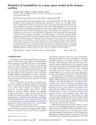
7. 0.04
Mean ξ
unstable poles, shown in Fig. 9 b , is located at a sinusoidal
(a)
0.03
1/2 λpeak wavelength somewhat shorter than half the peak wavelength.
Mean ξ As the sinusoidal wavelength of the gain variations is short-
0.02 ened, the number of peaks in the gain and thus reflection
sites along the cochlea increases, creating more unstable
0.01
poles. Even for sinusoidal periods less than half the peak
0
0.14 0.2 0.3 0.4 0.5 0.6 0.7 0.8 0.9 1
wavelength, the rate at which unstable poles are being gen-
erated per unit decrease in sin is still outpacing the rate at
which they are returning to stability; this explains the loca-
60
(b) tion of the peak in Fig. 9 b .
50
Funst count
40
30
C. Band-limited random gain distributions
20
10 Shera and Zweig’s 1993 theory of SOAE generation
0
assumes that the cochleae of normal-hearing humans contain
0.14 0.2 0.3 0.4 0.5 0.6 0.7 0.8 0.9 1
λsin [mm] a dense but random array of inhomogeneities. Each of these
place-fixed perturbations reflects energy from the forward
FIG. 9. Average undamping ratio a and number of unstable frequencies TW Talmadge et al., 1993; Shera and Zweig, 1993; Zweig
b for a sinusoidal distribution of gain with varying wavelength, sin. A and Shera, 1995 . In this section, the stability of cochlear
vertical line marks the location of half the wavelength of the TW at its peak. models with band-limited, spatially random gain distribu-
tions is used to approximate what is postulated to exist in a
human cochlea. A fifth order Butterworth filter was em-
B. Sinusoidal variations in gain
ployed to band-limit gain distributions in the wave number
A distribution of gain that is sinusoidal as a function of domain Lineton, 2001 . The low wave number cutoff fre-
position is of interest because its wave number spectrum is quency was fixed at the length of the cochlea itself, in order
concentrated at a single wave number, just as a sinusoidal to prevent any dc shifts in the gain. The high wave number
wave form that is a function time has a frequency spectrum cutoff frequency was initially set to 6.6 radians/ mm and
that is concentrated at a single frequency. This set of simu- slowly increased, thus generating cochlear models with suc-
lations follows the theory outlined by Strube 1989 , which cessively more densely spaced reflection sites. The average
assumes uniform corrugations in gain along the BM. A range filter bandwidths have been plotted below in terms of 2
of wavelengths was chosen for the sinusoidal variation gain times inverse wave number; this quantity has units of length
as a function of position along the cochlea, varying from mm and is directly comparable to the wavelength of the
1 mm down to 0.14 mm, the latter being the spatial Nyquist TW at its peak.
limit of the model. A 10% peak-to-peak variation in ampli- Figure 10 summarizes the results of simulations of 400
tude about nominal gain generated instabilities over most of different cochleae, each with unique, spatially random gain
this spatial range, while maintaining stability for sinusoidal distributions. The a panels show a typical stability plot
wavelengths greater than approximately 0.95 mm. from each group. The averaged power spectrum of the gain
Figure 9 summarizes the level of instability in these co- distributions is shown in the b panels, the two Roman nu-
chleae by plotting both the mean undamping ratio, , and the meral sets I and II having different high wave number low
number of unstable frequencies as a function of the gain’s wavelength cutoffs; the dashed vertical line represents half
sinusoidal wavelength. As expected, given the theories of the wavelength of the TW at its peak. A 5 mm sample of a
Strube 1989 , Shera and Zweig 1993 , and Zweig and gain distribution at this cutoff wavelength is inset. The c
Shera 1995 , the strongest instability occurred when the panels show the histograms of the average number of un-
wavelength of the sinusoid, sin, was approximately half the stable poles per cochlea, sorted into logarithmic frequency
peak wavelength; this value occurs at 0.44 mm in the model. bins. Figure 10 IIc demonstrates that a lower cutoff wave-
In addition, there was a region of greatly decreased instabil- length, and thus a more rapid spatial variation in gain, is
ity in the model, centered about a periodicity of approxi- necessary to generate instability at frequencies below 2 kHz.
mately one-fourth peak wavelength. This is thought to be due This is believed to be due to the lower level of enhancement
to destructive interference between the reflection sites, as the toward the apex of the cochlea and the lower magnitude of
backscattered wavelets are out of phase with each other the basal reflection coefficient in this frequency band.
given this spatial periodicity. The histogram of normalized spacings of adjacent un-
The locally jagged aspect of the mean undamping ratio stable frequencies per cochlea is shown in the d panels. The
curve in Fig. 9 a at approximately 0.75 mm is due to the data for the c and d panels are presented for all instabili-
periodic introduction of “new” unstable poles with low- ties gray, thick bars and also in a restricted range of
undamping ratios that are generated as the wavelength of the 0.5– 2 kHz thin, black bars . This smaller range represents
sinusoid is varied. The average undamping ratio peaks at the frequency bandwidth where the middle ear’s reverse-
approximately 0.5 mm, which is slightly longer than half the pressure transfer function is most efficient Puria, 2003 , and
peak wavelength for most of the length of the cochlea in this thus where one might expect the most SOAEs to be detected.
model. It is of note that the maximum in the total number of The results for cutoff = 0.19 mm Fig. 10 IId show a peak in
1074 J. Acoust. Soc. Am., Vol. 124, No. 2, August 2008 Ku et al.: Statistics of instabilities

8. Stability plot, Mean ξ = 0.012 Average spectrum, λcut−off = 0.78mm
3000 0
2000 −10
Magnitude [dB]
σ [sec ]
1000 −20
−1
0 −30
1.1
γ(x)
−1000 −40 1
−2000 −50 0.9
0 1 2 3 4 5
(I.a) (I.b) Position along the cochlea [mm]
−3000 −60
0 5 10 15 20 0.14 1 10 35
Frequency [kHz] λ [mm]
Histogram of unstable frequencies Histogram of normalised spacings
2.5 8 2
pair count
All Avg Funst pair count
All Unstable freqs., Funst (I.c) (I.d)
Avg. Funst count
2 0.5kHz < Funst < 2kHz
6 1.5
1.5
unst
4 1
Restricted F
1
2 0.5
0.5
0 0 0
0.5 1 2 5 10 20 2 3 5 7 10 20 30 50
(a) Frequency of instability [kHz] f/∆f
Stability plot, Mean ξ = 0.018 Average spectrum, λ = 0.19mm
cut−off
3000 0
2000 −10
Magnitude [dB]
σ [sec ]
1000 −20
−1
0 −30
1.1
γ(x)
−1000 −40 1
−2000 −50 0.9
0 1 2 3 4 5
(II.a) (II.b) Position along the cochlea [mm]
−3000 −60
0 5 10 15 20 0.14 1 10 35
Frequency [kHz] λ [mm]
Histogram of unstable frequencies Histogram of normalised spacings
2.5 8 2
pair count
All Avg Funst pair count
All Unstable freqs., Funst (II.c) (II.d)
count
2 0.5kHz < F < 2kHz
unst
6 1.5
1.5
unst
unst
4 1
Restricted F
Avg. F
1
2 0.5
0.5
0 0 0
0.5 1 2 5 10 20 2 3 5 7 10 20 30 50
(b) Frequency of instability [kHz] f/∆f
FIG. 10. The collected results from 2 200 cochlear models with randomly generated gain distributions. Each Roman numeral subset has been filtered with
a different cutoff wavelength: Ia – Id cutoff = 0.78 mm, IIa – IId cutoff = 0.19 mm. A peak-to-peak amplitude of 15% was applied to these gain distri-
butions. a A characteristic stability plot taken from the set. The average undamping ratio for that single case, , is given and superimposed dotted line . b
Averaged inverse wave number spectrum of the gain distributions. Half the peak wavelength is indicated by a dotted vertical line and the first 5 mm of a
characteristic gain distribution are inset. c Averaged histogram of all unstable frequencies per cochlea sorted in logarithmic frequency bins gray . The
instabilities occurring between 0.5 and 2 kHz are superimposed in thin, black bars. d Averaged histogram of normalized spacings f / f per cochlea in gray.
The histogram of spacings of unstable frequencies per cochlea occurring between 0.5 and 2 kHz is again superimposed in black. Note the different left- and
right-vertical scales.
the normalized spacing at f / f 15 in the frequency range Figure 11 summarizes data from the above calculations,
of 0.5– 2 kHz. These results are consistent with the Shera while also presenting data from many other simulations
and Zweig’s 1993 theory which assumes a dense array of which have different cutoff wavelengths and peak-to-peak
reflection sites, represented in these simulations by a low variations in gain. The mean unstable frequency count and
cutoff wavelength. the mean undamping ratio, , vary directly with the ampli-
J. Acoust. Soc. Am., Vol. 124, No. 2, August 2008 Ku et al.: Statistics of instabilities 1075

9. 0.025
(a) model. However, it is worth highlighting the similarities and
0.02 differences between measured data and these simulation re-
Mean ξ sults.
0.015
This model predicts that instabilities exist all along the
0.01
cochlea and across a wide band of frequencies, given a dense
0.005
array of inhomogeneities in the cochlea. In contrast, SOAEs
0
0.14 0.2 0.3 0.4 0.5 0.6 0.7 0.8 0.9 1
in normal-hearing individuals are only routinely detected be-
50
20% change in γ(x)
tween 0.5 kHz and 6 kHz Probst et al., 1991 . Even if in-
(b) 15% stabilities exist in all regions along the average human co-
Mean Funst count
40 10%
5.0%
2.5%
chlea, however, it is likely that only a subset of these will be
30 1.0%
0.5% detected in the ear canal. It is believed that the inefficient
20
reverse-transmission characteristics of the middle ear hinder
the detection of SOAEs outside of its best transmissibility
10
range, given its steep drop-off below and above resonance,
0 of approximately −40 dB/ decade. The limited bandwidth of
0.14 0.2 0.3 0.4 0.5 0.6 0.7 0.8 0.9 1
λ−3dB cutoff wavelength [mm] normally detected SOAEs is also potentially reduced by
physiological noise and the current limitations of sensor
FIG. 11. Variation of average undamping ratio a and total unstable pole technology. Just as improved measurement techniques have
count b with cutoff wavelength for five amplitudes of peak-to-peak ran- revealed increasingly sharp active BM enhancement through
dom variations in gain. At each amplitude, 20 cutoff wavelengths were each
applied to 200 models with randomly generated gain distributions. A total of
the years, refinements in recording technique have exposed a
28,000 stability tests were performed. higher prevalence of SOAEs in more recent studies Probst
et al., 1991; Penner and Zhang, 1997 .
The average number of unstable frequencies shown in
tude of the variation in x . This result is consistent with the Fig. 11 for a 10% peak-to-peak variation in gain is similar to
findings of Elliott et al. 2007 . In contrast to the sinusoidal the maximum number of emissions detected in a single ear,
case see Fig. 9 , no distinct notch in either the average un- some in excess of 30 SOAEs Talmadge et al., 1993 . It has
damping ratio or the number of instabilities is apparent at a been shown that the level and number of instabilities in the
cutoff wavelength of approximately one-quarter of the peak state space model depend on the amplitude of the variations
wavelength. In the sinusoidal simulations, all of the spatial in BM impedance and the spatial density of the inhomoge-
spectral energy was concentrated at a particular wave num- neities. When nonlinear effects are incorporated into time-
ber; this potentially generated strong, destructive interference domain simulations, it is anticipated that the total number of
when the sinusoidal wavelength was one-quarter the peak instabilities may differ from those predicted by linear stabil-
wavelength. The spectral energy in the random spatial varia- ity analysis.
tions in gain is comparatively much more diffuse, perhaps It has been demonstrated by numerous experimentalists
reducing the amount of both constructive and destructive in- e.g., Zwicker and Schloth, 1984 that externally applied
terferences. The statistics of the spacings of instabilities is stimuli can frequency-lock, phase-synchronize, suppress, or
thus largely independent of the exact form of the spatial otherwise affect a SOAE. Some modelers have used Van der
variations, provided they have a significant component at the Pol oscillators to account for these phenomena Bialek and
wave number corresponding to one-half peak. Peak-to-peak Wit, 1984; Wit, 1986; van Hengel et al., 1996 . Further work
variations in x as small as 0.5% can give rise to instabili- is needed to examine the nonlinear interaction of limit cycles
ties, provided cutoff is less than approximately 0.5 mm, near and external stimuli in the state space model presented here.
the half peak wavelength. The current linear model predicts a distribution of un-
stable frequency spacings that is similar to physiologically
compiled data in several respects. Although the current mod-
IV. DISCUSSION el’s results do not accurately match the observed variation in
SOAE spacings with frequency Shera, 2003 , the spacing
The findings of this paper, based on a numerical model results presented in Fig. 10 IId are consistent with the pre-
of the human cochlea, are consistent with the multiple- dictions shown in Fig. 5 d . Furthermore, the peak in the
reflection theory of Zweig and Shera 1995 . The state space normalized spacings of Fig. 10 IId is correctly located at the
formulation is able to predict the frequencies at which a lin- PMD when sufficient spectral content is present in the inho-
ear, active cochlear model will become unstable. Elliott et al. mogeneities at half the peak wavelength, as predicted by
2007 presented a nonlinear time-domain simulation dem- Zweig and Shera 1995 .
onstrating that an isolated unstable pole will evolve into a When the current understanding regarding hearing sen-
limit cycle within the cochlea at the expected frequency. Di- sitivity, the various forms of OAEs and pathology are com-
rect measurements in animals have shown that spontaneous bined, a convincing picture regarding the generation of
basilar membrane oscillation is associated with SOAEs in SOAEs begins to emerge. As many authors have pointed out,
the ear canal Nuttall et al., 2004 . Consequently, compari- SOAEs in humans appear to be a natural by-product of the
sons are drawn in this paper between measured SOAE char- species’ sharply tuned sense of hearing. Normal hearing in-
acteristics and the instabilities generated in the cochlear dividuals that do not exhibit SOAEs typically have an audio-
1076 J. Acoust. Soc. Am., Vol. 124, No. 2, August 2008 Ku et al.: Statistics of instabilities

10. gram which underperforms those with SOAEs by approxi- ˙
x N t = A Nx N t + B N p N t , A1
mately 3 dB in the standard 1 – 6 kHz range McFadden and
Mishra, 1993 . Pélanová et al. 2007 also reported that the where the boundary condition is now taken to be a mass-
high-frequency audiogram of normal-hearing children with- damper system, so that
out SOAEs underperformed those with SOAEs by approxi- ˙
xN t = wN t wN t T
, A2
mately 5 dB through the 10– 16 kHz range. In the “laser-
cochlea” theory of OAE generation, it is the portion of the − CH
cochlea basal to the reflection site that is crucial to sustaining 0
AN = MH , A3
the limit cycle oscillation. If the losses in this region are not
overcome by the active enhancement provided by the outer 1 0
hair cells, no spontaneous emission can occur. and
T
V. CONCLUSIONS 1
BN = 0 . A4
MH
Simulations using the state space model of the human
cochlea show patterns of SOAE production that can be ex- In order to incorporate this change into the macromechanical
plained by Zweig and Shera’s 1995 theory. As demon- formulation, it was necessary to insert an additional term in
strated by the step change in gain, only frequencies with a the finite difference fluid-coupling matrix, F, such that it is
TW that undergoes an integer round-trip phase change be- still invertible. The expanded matrices represented in Eq. 1
tween the middle ear boundary and the inhomogeneity will of this work now become
become unstable. Instabilities are detected along the entire
cochlea given spatially random changes in gain, but it is − 0
believed that only a subset of these unstable frequencies be- H H
come measurable as SOAEs due to the middle ear’s ineffi- 1 −2 1
cient reverse transmission characteristics. The spectral con- 0 1 −2 1
tent of the inhomogeneities in the BM impedance also has a H
strong impact upon the level and frequency spacings of the 2
2
resultant instabilities. 1 −2 1 0
A 10% variation in gain as a function of position gener- 1 −2 1
ated the most instability in the model when a sinusoidal in- 2
homogeneity with a wavelength roughly equal to half the 0 − +
H H H2
wavelength of the TW at its peak was applied; instability was
eliminated when the sinusoid’s wavelength was reduced to p1 t ¨
wSR t ¨
wSO t
roughly one-fourth the wavelength of the TW at its peak. p2 t ¨
w2 t 0
When random inhomogeneities are simulated, the expected
PMD between adjacent unstable frequencies is strongly ex-
pressed in the results only when there is sufficient spectral ] − ] = , A5
content at one-half the wavelength of the TW at its peak. ]
Nonlinear time-domain simulations, such as those intro-
duced in Elliott et al. 2007 , are expected to provide a pN−1 t ¨
wN−1 t
method of explaining the more subtle interactions that exist pN t ¨
wN t 0
in human cochleae due to multiple instabilities and exter-
nally applied stimuli. However, it is clear that this linear where H is the height of the channel, is the density of the
model can provide a great deal of insight into the mecha- fluid, and is the length of a cochlear segment. The physical
nisms underlying the generation of SOAEs as numerical re- meaning of this additional term in the fluid-coupling matrix
sults presented here are in good agreement with the theory of can be determined by relating this revised equation to the
Zweig and Shera 1995 . boundary condition at the apex.
The last row in Eq. A5 represents the helicotrema
ACKNOWLEDGMENTS boundary condition and can be written as
2
The authors would like to thank Dr. Sunil Puria for shar- H
2 pN−1 − + ¨
pN = 2 wN , A6
ing his research data, and two anonymous reviewers for their H H H2
helpful comments and suggestions. This work was partially
where pN−1 and pN are the pressures adjacent to and at the
supported by a Fulbright Postgraduate Award. ¨
helicotrema, and wN represents the “effective” helicotrema
acceleration. Rewriting Eq. A6 gives
APPENDIX: HELICOTREMA BOUNDARY CONDITION
pN−1 − pN 1
The structure of the noncoupled micromechanical matri- ¨
= 2 wN + pN . A7
H
ces is identical to Elliott et al. 2007 , except at the heli-
cotrema for which However, the physical boundary condition is defined as
J. Acoust. Soc. Am., Vol. 124, No. 2, August 2008 Ku et al.: Statistics of instabilities 1077