Fl3410191025

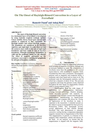
Ramesh Chand and Ankuj Bala / International Journal of Engineering Research and
Applications (IJERA) ISSN: 2248-9622 www.ijera.com
Vol. 3, Issue 4, Jul-Aug 2013, pp.1019-1025
1019 | P a g e
On The Onset of Rayleigh-Bénard Convection in a Layer of
Ferrofluid
Ramesh Chand1
and Ankuj Bala2
1
Department of Mathematics, Government College, Dhaliara (Kangra), Himachal Pradesh, INDIA
2
Department of Mathematics, Himachal Institute of Engineering and Technology, Shahpur, Himachal
Pradesh, INDIA
ABSTRACT
The onset of Rayleigh-Bénard convection
in a horizontal layer of ferrofluid is investigated
by using Galerkin weighted residuals method.
Linear stability theory based upon normal mode
analysis is employed to find expressions for
Rayleigh number and critical Rayleigh number.
The boundaries are considered to be free-free,
rigid-free and rigid-rigid. It is also observed that
the system is more stable in the case of rigid-rigid
boundaries and least stable in case of free-free
boundaries. ‘Principle of exchange of stabilities’ is
valid and the oscillatory modes are not allowed.
The effect of magnetic parameter on the
stationary convection is investigated graphically
for all types of boundary conditions.
Key words: Ferrofluid, Convection, Magnetic
thermal Rayleigh number, Galerkin method, Prandtl
number.
Nomenclature
a wave number
B magnetic induction
g acceleration due to gravity
H magnetic field intensity
k thermal conductivity
K1 pyomagnetic coefficient
M magnetization
M1 buoyancy magnetization
M3 magnetic parameter
N magnetic thermal Rayleigh number
n growth rate of disturbances
p pressure (Pa)
Pr Prandtl number
q fluidvelocity
R Rayleigh number
Rc critical Rayleigh number
t time
T temperature
Ta average temperature
u, v, w fluid velocity components
(x, y, z) space co-ordinates
Greek symbols
α thermal expansion coefficient
β uniform temperature gradient
μo magnetic permeability
μ viscosity
ρ density of the fluid
(ρc ) heat capacity of fluid
κ thermal diffusivity
φ' perturbed magnetic potential
ω dimensional frequency
χ magnetic susceptibility
Superscripts
' non dimensional variables
' ' perturbed quantity
Subscripts
0 lower boundary
1 upper boundary
H horizontal plane
I. Introduction
Ferrofluid formed by suspending submicron
sized particles of magnetite in a carrier medium such
as kerosene, heptanes or water. The attractiveness of
ferrofluids stems from the combination of a normal
liquid behavior with sensitivity to magnetic fields.
Ferrofluid has three main constituents: ferromagnetic
particles such as magnetite and composite ferrite, a
surfactant, and a base liquid such as water or oil. The
surfactant coats the ferromagnetic particles, each of
which has a diameter of about 10 nm. This prevents
coagulation and keeps the particles evenly dispersed
throughout the base liquid. Its dispersibility remains
stable in strong magnetic fields.
Ferromagnetic fluid has wide ranges of
applications in instrumentation, lubrication,
printing, vacuum technology, vibration damping,
metals recovery, acoustics and medicine, its
commercial usage includes vacuum feed through for
semiconductor manufacturing in liquid-cooled
loudspeakers and computer disk drives etc. Owing
the applications of the ferrofluid its study is
important to the researchers. A detailed account on
the subject is given in monograph has been given by
Rosensweig (1985). This monograph reviews
several applications of heat transfer through
ferrofluid. One such phenomenon is enhanced
convective cooling having a temperature-dependent
magnetic moment due to magnetization of the fluid.
This magnetization, in general, is a function of the
magnetic field, temperature, salinity and density of
the fluid. In our analysis, we assume that the
magnetization is aligned with the magnetic field.

1020 | P a g e
Convective instability of a ferromagnetic fluid for a
fluid layer heated from below in the presence of
uniform vertical magnetic field has been considered
by Finlayson (1970). He explained the concept of
thermo-mechanical interaction in ferromagnetic
fluids. Thermoconvective stability of ferromagnetic
fluids without considering buoyancy effects has
been investigated by Lalas and Carmi (1971).
Linear and nonlinear convective instability of a
ferromagnetic fluid for a fluid layer heated from
below under various assumptions is studied by many
authors Shliomis (2002), Blennerhassett et.al.(1991),
Gupta and Gupta (1979), Stiles and Kagan (1990),
Sunil et.al. (2005, 2006), Sunil, Mahajan (2008),
Venkatasubramanian and Kaloni (1994), Zebib
(1996), Mahajan (2010). However, a limited effort
has been put to investigate the instability in rigid-
rigid and rigid-free boundaries. In this paper an
attempt has been made to study the linear
convective instability of a ferromagnetic fluid for a
fluid layer heated from below by Galerkin weighted
residuals method for all type of boundary
conditions.
II. Mathematical Formulation of the
Problem
Consider an infinite, horizontal layer of an
electrically non-conducting incompressible
ferromagnetic fluid of thickness ‘d’, bounded by
plane z = 0 and z = d. Fluid layer is acted upon by
gravity force g (0, 0, -g) and a uniform magnetic field
kˆHext
0H acts outside the fluid layer. The layer is
heated from below such that a uniform temperature
gradient 






dz
dT
is to be maintained. The
temperature T at z = 0 taken to be T0 and T1 at z = d,
(T0 > T1) as shown in Fig.1.
Fig.1 Geometrical configuration of the problem
The mathematical governing equations
under Boussinesq approximation for the above model
(Finlayson (1970), Resenweig (1997), and Mahajan
(2010) are:
0. q , (1)
 HMqg
q
 .p
dt
d
0
2
00 , (2)
    TkT.qC
dt
dT
C 2
f0f0   , (3)
Maxwell’s equations, in magnetostatic limit:
0. B , 0 H ,  .MHB 0  (4)
The magnetization has the relationship
    1100 TTKHHM
H

H
M . (5)
The density equation of state is taken as
  aTT1   . (6)
Here ρ, ρ0, q, t, p, μ, μ0, H, B, C0, T, M, K1,
and α are the fluid density, reference density,
velocity, time, pressure, dynamic viscosity (constant),
magnetic permeability, magnetic field, magnetic
induction, specific heat at constant pressure,
temperature, magnetization, thermal conductivity and
thermal expansion coefficient, Ta is the average
temperature given by 




 

2
TT
T 10
a , HH ,
MM and  a00 T,HMM  . The magnetic
susceptibility and pyomagnetic coefficient are
defined by
aT,HH
M









 and
aT,H
1
T
M
K









 respectively.
Since the fluid under consideration is
confined between two horizontal planes z = 0 and z =

1021 | P a g e
d, on these two planes certain boundary conditions
must be satisfied. We assume the temperature is
constant at z = 0, z = d, thus boundary conditions
[Chandrasekhar (1961), Kuznetsov and Nield (2010)]
are
0zat0D,TT0,
z
w
d
z
w
0,w 02
2
1 





 ,
dzat0D,TT0,
z
w
d
z
w
0,w 12
2
2 





 . (7)
The parameters λ1 and λ2 each take the
value 0 for the case of a rigid boundary and ∞ for a
free boundary.
2.1 Basic Solutions
The basic state is assumed to be a quiescent
state and is given by
    0w,v,uqw,v,uq b 
,
 zpp b
,
  ab TzzTT 
,
 
kˆ
1
TTK
HH ab1
b 







  ,
 
kˆ
1
TTK
MM ab2
b 







  ,
extHMH   . (8)
2.2 The Perturbation Equations
We shall analyze the stability of the basic state by
introducing the following perturbations:
qqq b
 ,   pzpp b  ,    zTT b ,
  HzHH b     MzMM b
 (9)
where q′(u,v,w), δp, θ, H′(H'1,H'2,H'3) and
M′(M'1,M'2,M'3) are perturbations in velocity,
pressure, temperature, magnetic field and
magnetization. These perturbations are assumed to be
small and then the linearized perturbation equations
are
0. q , (10)
  













 kˆKkˆ
z
1
1
K
kˆgp
t
1
11
0
2 
 q
q
(11)
w
t
2



, (12)
z
K
zH
M
H
M
1 12
1
2
0
0
1
2
0
0


















(13)
where  and1H is the perturbed
magnetic potential and
 f00cρ
k
κ  is thermal
diffusivity of the fluid.
And boundary conditions are
0zat0D,TT0,
z
w
d
z
w
0,w 02
2
1 





 ,
dzat0D,TT0,
z
w
d
z
w
0,w 12
2
2 






(14)
We introduce non-dimensional variables as
,
d
z,y,x
)z,y,x( 




 
 ,
d

 qq
,t
d
κ
t 2
 ,p
κ
d
p
2


 ,
d


 
12
1
1
dK
1



 .
There after dropping the dashes ( '' ) for simplicity.
Equations (10)-(14), in non dimensional form can be
written as
0. q , (15)
  kˆ
z
RMkˆM1Rp
tPr
1 1
11
2





q
q
,
(16)
w
t
2



, (17)
 
zz
1MM 2
1
2
31
2
3






. (18)
where non-dimensional parameters are:
ρκ
μ
Pr  is Prandtl number;
μκ
dgαρ
R
4
0 
 is
Rayleigh number;
 1g
K
M
0
2
10
1


 measure
the ratio of magnetic to gravitational forces,
 1μκ
dK
RMN
422
10
1


 is magnetic thermal
Rayleigh number;
 1
H
M
1
M
0
0
3








 measure the
departure of linearity in the magnetic equation of
state and values from one  00 HM  higher
values are possible for the usual equation of state.
The dimensionless boundary conditions are
0zat0Dφ,1T0,
z
w
z
w
0,w 2
2
1 






and 1zat0Dφ0T0,
z
w
z
w
0,w 2
2
2 






. (19)

1022 | P a g e
Operating equation (10) with curl,.curlkˆ we get
  1
2
H1
2
H1
42
DRMM1Rww
tPr
1



.
(20)
where ,2
H is two-dimensional Laplacian operator
on horizontal plane.
III. Normal Mode Analysis
Analyzing the disturbances of normal modes
and assume that the perturbation quantities are of the
form
     ntyikxikexpΦ(z)Θ(z),W(z),φ,w, yx1 
,
(21)
where, kx, ky are wave numbers in x- and y- direction
and n is growth rate of disturbances.
Using equation (21), equations (20) and (17) - (18)
becomes
    0,DΦRMaΘM1RaWaD
Pr
n
aD 1
2
1
22222







(22)
  0,ΘnaDW 22
 (23)
  0MaDD 3
22
 . (24)
where
dz
d
D  , and a2
= k2
x+ k2
y is dimensionless
the resultant wave number.
The boundary conditions of the problem in view of
normal mode analysis are
(i) when both boundaries free
0,1zat0D,00,WD0,W 2
 .
(25a)
(ii) when both boundaries rigid
0,1zat0D,00,DW0,W  .
(25b)
(ii) when lower rigid and upper free boundaries
0,zat0D,00,DW0,W 
1zat0D,00,WD0,W 2
 .
(25c)
IV. Method of solution
The Galerkin weighted residuals method is
used to obtain an approximate solution to the system
of equations (22) – (24) with the corresponding
boundary conditions (25). In this method, the test
functions are the same as the base (trial) functions.
Accordingly W, Θ and Φ are taken as
 

n
1p
pp
n
1p
pp
n
1p
pp DCDΦ,B,WAW .
(26)
Where Ap, Bp and Cp are unknown coefficients, p =1,
2, 3,...N and the base functions Wp, Θp and DΦp are
assumed in the following form for free-free, rigid-
rigid and rigid-free boundaries respectively:
,zpπosCDΦz,πposCΘ,zpπosCW ppp 
(27)
,zzD,zz,zz2zW 1pp
p
1pp
p
3p2p1p
p


(28)
    1pp
p
1pp
p
p2
p zzD,zz,z22pz1zW 

.
(29)
such that Wp, Θp and Φp satisfy the corresponding
boundary conditions. Using expression for W, Θ and
DΦ in equations (22) – (24) and multiplying first
equation by Wp second equation by Θp and third by
DΦp and integrating in the limits from zero to unity,
we obtain a set of 3N linear homogeneous equations
in 3N unknown Ap, Bp and Cp; p =1,2,3,...N. For
existing of non trivial solution, the vanishing of the
determinant of coefficients produces the
characteristics equation of the system in term of
Rayleigh number R.
V. Linear Stability Analysis
5.1 Solution for free boundaries:
We confined our analysis to the one term
Galerkin approximation; for one term Galerkin
approximation, we take N=1, the appropriate trial
function are given as
,zπcosDΦz,πcosΘ,zπcosW ppp  (30)
which satisfies boundary conditions
0zat0D,00,WD0,W 2
 and
1zat0D,00,WD0,W 2
 . (31)
Using trial function (30) boundary conditions (31) we
get the expression for Rayleigh number R as:
    
 31
2
3
222
222222
3
22
MMaMaa
ana
Pr
n
aMa
R









. (32)
For neutral stability, the real part of n is zero. Hence
we put n = iω, in equation (32), where ω is real and is
dimensionless frequency, we get
    
 31
2
3
222
222222
3
22
MMaMaa
aia
Pr
i
aMa
R






 


. (33)
Equating real and imaginary parts, we get
21 iR  , (34)
where

1023 | P a g e
    
 31
2
3
222
2
22222
3
22
1
MMaMaa
Pr
aaMa
Δ






 


, (35)
and
  
 31
2
3
222
22
3
22
2
MMaMaa
Pr
1
1aMa
Δ








 . (36)
Since R is a physical quantity, so it must be
real. Hence, it follow from the equation (34) that
either ω = 0 (exchange of stability, steady state) or Δ2
= 0 (ω # 0 overstability or oscillatory onset).
But Δ2 # 0, we must have ω = 0, which means that
oscillatory modes are not allowed and the principle of
exchange of stabilities is satisfied. This is the good
agreement of the result as obtained by Finlayson
(1970).
(a) Stationary Convection
Consider the case of stationary convection
i.e., ω = 0, from equation (33), we have
   
 31
2
3
222
3
22322
MMaMaa
Maa
R


 . (37)
This is the good agreement of the result as obtained
by Finlayson (1970).
In the absence of magnetic parameters M1=M3=0, the
Rayleigh number R for steady onset is given by
 
2
322
a
a
R

 . (38)
Consequently critical Rayleigh number is given by
4
27
Rc
2

 .
This is exactly the same the result as
obtained by Chandrasekhar (1961) in the classical
Bénard problem.
5.2 Solution Rigid-Rigid Boundaries
We confined our analysis to the one term
Galerkin approximation; the appropriate trial function
for rigid-rigid boundary conditions is given by
     ,z1zD,z1z,z1zW pp
22
p 
(39)
which satisfied boundary conditions
0zat0D,00,DW0,W  and
1zat0D,00,DW0,W  . (40)
Using trial function (39) boundary
conditions (40) we get the expression for Rayleigh
number R as:
     





























421313
10
Pr
1
12504244213
27
28
R
31
2
3
2
224
3
2
2
MMaMa
nanaaMa
a
. (41)
For neutral stability, the real part of n is zero. Hence
we put n = iω, in equation (41), we get
     



























42MMa13Ma13
i10a
Pr
1
12i504a24a42Ma13
a27
28
R
31
2
3
2
224
3
2
2
. (42)
Equating real and imaginary parts, we get
43 iR  , (43)
where
    



























42MMa13Ma13
Pr
1
1210a504a24a42Ma13
a27
28
Δ
31
2
3
2
2224
3
2
23
, (44)
and
     



























42MMa13Ma13
10a
Pr
1
12504a24a42Ma13
a27
28
Δ
31
2
3
2
224
3
2
24
. (45)
Since R is a physical quantity, so it must be
real. Hence, it follow from the equation (43) that
either ω = 0 (exchange of stability, steady state) or Δ2
= 0 (ω # 0 overstability or oscillatory onset).
But Δ2 # 0, we must have ω = 0, which means that
oscillatory modes are not allowed and the principle of
exchange of stabilities is satisfied for rigid –rigid
boundaries.
(b) Stationary Convection
Consider the case of stationary convection
i.e., ω = 0, from equation (42), we have
   









42MMa13Ma13
42Ma1310a504a24a
a27
28
R
31
2
3
2
3
2224
2
. (46)
In the absence of magnetic parameters
M1=M3=0, the Rayleigh number R for steady onset is
given by
  10a504a24a
a27
28
R 224
2
 . (47)

1024 | P a g e
This is exactly the same the result as obtained by
Chandrasekhar (1961) in the classical Bénard
problem for rigid -rigid boundaries.
5.3 Solution Rigid-Free Boundaries
The appropriate trial function to the one term
Galerkin approximation for rigid-free boundary
conditions is given by
      z1zD,z1z,z23z1zW pp
2
p 
, (48)
which satisfied boundary condition
0zat0D,00,DW0,W  and
1zat0D,00,WD0,W 2
 . (49)
It is observed that oscillatory modes are not
allowed and the principle of exchange of stabilities is
satisfied for rigid -free boundaries.
The eigenvalue equation for stationary case takes the
form
   
42MMa13Ma13
10a4536a432a1942Ma13
a507
28
R
31
2
3
2
224
3
2
2



. (50)
In the absence of magnetic parameter M1=M3=0, the
Rayleigh number R for stationary convection is given
by
  10a4536a432a19
a507
28
aR 224
2

. (51)
This is the good agreement of the result as
obtained by Chandrasekhar (1961) in the classical
Bénard problem.
VI. Results and Discussion
Expressions for Stationary convection Rayleigh
number are given by equations (37), (46) and (50) for
the case of free-free, rigid-rigid and rigid-free
boundaries. It is observed that oscillatory modes not
allowed for layer of ferrofluid heated from below.
We have discussed the results numerically and
graphically. The stationary convection curves in (R,
a) plane for various values of magnetization M3 and
fixed values of M1=1000, other parameters as shown
in Fig. 2. It is clear that the linear stability criteria to
be expressed in thermal Rayleigh number, below
which the system is stable and unstable above. It has
been found that the Rayleigh number decrease with
increase in the value of magnetization M3 thus
magnetization M3 destabilizing effect on the system.
It is also found that stability of fluid layer in most
stable in rigid-rigid boundaries and least stable free-
free boundaries. It is also observed that oscillatory
modes are not allowed and the principle of exchange
of stabilities is satisfied for all type of boundary
conditions i.e free-free, rigid-rigid and rigid -free
boundaries.
Fig.2 Variation of critical Rayleigh number R with wave number a for different value of magnetization M
0
5
10
15
20
25
30
35
0.35 0.85 1.35 1.85 2.35
RayleighNumber
Wave Number
Rigid-Rigid
Boundries
Rigid-Free
Boundries
Free-Free
Boundries
M3=4
M3=8
M3=6

1025 | P a g e
VII. Conclusions
A linear analysis of thermal instability for
ferrofluid for free-free, rigid-rigid and rigid -free
boundaries is investigated. Galerkin-type weighted
residuals method is used for the stability analysis.
The behavior of magnetization on the onset of
convection analyzed for all type of boundaries.
Results has been depicted graphically.
The main conclusions are as follows:
1. For the case of stationary convection, the
magnetization parameter destabilized the fluid
layer for all type of boundary conditions.
2. The ‘principle of exchange of stabilities’ is valid
for all type of boundary conditions.
3. The oscillatory modes are not allowed for the
ferromagnetic fluid heated from below.
4. It is also found that stability of fluid layer in
most stable in rigid-rigid boundaries and least
stable in free-free boundary conditions.
References
[1] Blennerhassett, P. J., Lin, F. & Stiles, P. J.:
Heat transfer through strongly magnetized
ferrofluids, Proc. R. Soc. A 433, 165-177,
(1991).
[2] Chandrasekhar, S.: Hydrodynamic and
hydromagnetic stability, Dover, New York
(1981)
[3] Finlayson, B.A.: Convective instability of
ferromagnetic fluids. J. Fluid Mech. 40, 753-
767 (1970).
[4] Gupta, M.D., Gupta, A.S.: Convective
instability of a layer of ferromagnetic fluid
rotating about a vertical axis, Int. J. Eng.
Sci. 17, 271-277, (1979).
[5] Kuznetsov, A. V., Nield, D. A.: Thermal
instability in a porous medium layer
saturated by a nanofluid: Brinkman Model,
Transp. Porous Medium, 81, 409-422,
(2010).
[6] Lalas, D. P. & Carmi, S.: Thermoconvective
stability of ferrofluids. Phys. Fluids 14, 436-
437, (1971).
[7] Mahajan A. : Stability of ferrofluids: Linear
and Nonlinear, Lambert Academic
Publishing, Germany, (2010).
[8] Rosensweig, R.E.: Ferrohydrodynamics,
Cambridge University Press, Cambridge
(1985).
[9] Shliomisa, M.I and Smorodinb, B.L.:
Convective instability of magnetized
ferrofluids, Journal of Magnetism and
Magnetic Materials, 252,197-202, (2002).
[10] Stiles, P. J. & Kagan, M. J.:Thermo-
convective instability of a horizontal layer of
ferrofluid in a strong vertical magnetic field,
J. Magn. Magn. Mater, 85, 196-198, (1990).
[11] Sunil, Sharma, D. and Sharma, R. C.: Effect
of dust particles on thermal convection in
ferromagnetic fluid saturating a porous
medium, J. Magn. Magn. Mater. 288, 183-
195, (2005).
[12] Sunil, Sharma, A. and Sharma, R. C.: Effect
of dust particles on ferrofluid heated and
soluted
[13] from below, Int. J. Therm. Sci. 45, 347-358,
(2006).
[14] Sunil, Mahajan, A.: A nonlinear stability
analysis for magnetized ferrofluid heated
from below. Proc. R. Soc. A 464, 83-98
(2008).
[15] Venkatasubramanian, S., Kaloni, P.N.:
Effects of rotation on the thermoconvective
instability of a horizontal layer of
ferrofluids. Int. J. Eng. Sci. 32, 237–256
(1994).
[16] Zebib, A : Thermal convection in a magnetic
fluid, J. Fluid Mech., 32 , 121-136, (1996).

Fl3410191025

Recommended

Recommended

More Related Content

What's hot

What's hot (18)

Viewers also liked

Viewers also liked (20)

Similar to Fl3410191025

Similar to Fl3410191025 (20)

Recently uploaded

Recently uploaded (20)

Fl3410191025