This document discusses centroids and centers of mass. It defines the centroid of a set of points as the point where the sum of first moments is equal to zero. The position vector of the centroid is given by the weighted average of the position vectors of the individual points. Similarly, the center of mass of a system of particles is the weighted average of their position vectors, where the weights are the particle masses. Methods for finding the centroid of curves, surfaces, solids and continuous bodies are presented using integrals. The first moment of an area is introduced and related to the area centroid. Properties of centroids and centers of mass, such as their dependence on reference frames and behavior under decomposition, are covered.

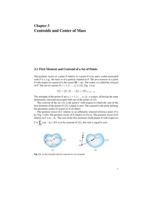
1. Chapter 3
Centroids and Center of Mass
3.1 First Moment and Centroid of a Set of Points
The position vector of a point P relative to a point O is rP and a scalar associated
with P is s, e.g., the mass m of a particle situated at P. The first moment of a point
P with respect to a point O is the vector M = s rP . The scalar s is called the strength
of P. The set of n points Pi , i = 1, 2, . . . , n, is {S}, Fig. 3.1(a)
{S} = {P1 , P2 , . . . , Pn } = {Pi }i=1,2,...,n .
The strengths of the points Pi are si , i = 1, 2, . . . , n, i.e., n scalars, all having the same
dimensions, and each associated with one of the points of {S}.
The centroid of the set {S} is the point C with respect to which the sum of the
first moments of the points of {S} is equal to zero. The centroid is the point defining
the geometric center of system or of an object.
The position vector of C relative to an arbitrarily selected reference point O is
rC , Fig. 3.1(b). The position vector of Pi relative to O is ri . The position vector of Pi
relative to C is ri − rC . The sum of the first moments of the points Pi with respect to
n
C is
∑ si (ri − rC ). If C is to be centroid of {S}, this sum is equal to zero
i=1
P1 ( s 1 )
P2 ( s 2 )
C
Pi ( si )
Pn ( s n )
{S}
rC
ri
Pi ( s i )
{S}
O
(a)
(b)
Fig. 3.1 (a) Set of points and (b) centroid of a set of points
1

2. 2
3 Centroids and Center of Mass
n
n
n
i=1
i=1
i=1
∑ si (ri − rC ) = ∑ si ri − rC ∑ si = 0.
The position vector rC of the centroid C, relative to an arbitrarily selected reference
point O, is given by
n
∑ si ri
rC =
i=1
n
.
∑ si
i=1
n
If ∑ si = 0 the centroid is not defined. The centroid C of a set of points of given
i=1
strength is a unique point, its location being independent of the choice of reference
point O.
The cartesian coordinates of the centroid C(xC , yC , zC ) of a set of points Pi , i =
1, . . . , n, of strengths si , i = 1, . . . , n, are given by the expressions
n
n
∑ si xi
xC =
i=1
n
∑ si
i=1
n
∑ si yi
, yC =
i=1
n
∑ si zi
, zC =
∑ si
i=1
i=1
n
.
∑ si
i=1
The plane of symmetry of a set is the plane where the centroid of the set lies, the
points of the set being arranged in such a way that corresponding to every point on
one side of the plane of symmetry there exists a point of equal strength on the other
side, the two points being equidistant from the plane.
A set {S } of points is called a subset of a set {S} if every point of {S } is a point
of {S}. The centroid of a set {S} may be located using the method of decomposition:
• divide the system {S} into subsets;
• find the centroid of each subset;
• assign to each centroid of a subset a strength proportional to the sum of the
strengths of the points of the corresponding subset;
• determine the centroid of this set of centroids.
3.2 Centroid of a Curve, Surface, or Solid
The position vector of the centroid C of a curve, surface, or solid relative to a point
O is

3. 3.2 Centroid of a Curve, Surface, or Solid
3
r dτ
τ
rC =
,
(3.1)
dτ
τ
where, τ is a curve, surface, or solid, r denotes the position vector of a typical point
of τ, relative to O, and dτ is the length, area, or volume of a differential element of
τ. Each of the two limits in this expression is called an “integral over the domain τ
(curve, surface, or solid).” The integral
dτ gives the total length, area, or volume
τ
of τ, that is
dτ = τ.
τ
The position vector of the centroid is
rC =
1
τ
r dτ.
τ
Let ı, j, k be mutually perpendicular unit vectors (cartesian reference frame) with
the origin at O. The coordinates of C are xC , yC , zC and
rC = xC ı + yC j + zC k.
It results that
xC =
1
τ
x dτ, yC =
τ
1
τ
y dτ, zC =
τ
1
τ
(3.2)
z dτ.
τ
The coordinates for the centroid of a curve L, Fig. 3.2, is determined by using three
scalar equations
x dL
xC =
L
y dL
, yC =
L
dL
L
C
dA
y
z
O
L
L
dL
.
(3.3)
dL
L
dL
r
z dL
, zC =
L
dV
C
C
A
V
x
Fig. 3.2 Centroid of a curve L, an area A, and a a volume V

4. 4
3 Centroids and Center of Mass
The centroid of an area A, Fig. 3.2, is
x dA
xC =
A
y dA
A
, yC =
z dA
, zC =
dA
A
dA
A
,
(3.4)
.
(3.5)
dA
A
A
and similarly the centroid of a volume V , Fig. 3.2, is
y dV
x dV
xC =
V
V
, yC =
z dV
, zC =
dV
V
dV
V
dV
V
V
For a curved line in the xy plane the centroidal position is given by
x dl
xC =
y dl
, yC =
L
L
,
(3.6)
where L is the length of the line. Note that the centroid C is not generally located
along the line. A curve made up of simple curves is considered. For each simple
curve the centroid is known. The line segment Li , has the centroid Ci with coordinates xCi , yCi , i = 1, ...n. For the entire curve
n
n
∑ xCi Li
xC =
i=1
L
∑ yCi Li
, yC =
i=1
n
, where L = ∑ Li .
L
i=1
3.3 Mass Center of a Set of Particles
The mass center of a set of particles {S} = {P1 , P2 , . . . , Pn } = {Pi }i=1,2,...,n is the
centroid of the set of points at which the particles are situated with the strength of
each point being taken equal to the mass of the corresponding particle, si = mi , i =
1, 2, . . . , n. For the system system of n particles in Fig. 3.3, one can write
n
n
∑ mi
i=1
rC = ∑ mi ri ,
i=1
and the mass center position vector is
n
∑ mi ri
rC =
i=1
M
,
(3.7)

5. 3.4 Mass Center of a Curve, Surface, or Solid
z
Pn
P2
m2
r2
mn
5
C
rC
rn
y
O
r1
x
P1
m1
Fig. 3.3 Mass center position vector
where M is the total mass of the system.
3.4 Mass Center of a Curve, Surface, or Solid
To study problems concerned with the motion of matter under the influence of
forces, i.e., dynamics, it is necessary to locate the mass center. The position vector of the mass center C of a continuous body τ, curve, surface, or solid, relative to
a point O is
r ρ dτ
rC =
τ
=
ρ dτ
1
m
r ρ dτ,
(3.8)
τ
τ
or using the orthogonal cartesian coordinates
xC =
1
m
x ρ dτ, yC =
τ
1
m
y ρ dτ, zC =
τ
1
m
z ρ dτ,
τ
where, ρ is the mass density of the body: mass per unit of length if τ is a curve,
mass per unit area if τ is a surface, and mass per unit of volume if τ is a solid, r
is the position vector of a typical point of τ, relative to O, dτ is the length, area, or
volume of a differential element of τ, m = τ ρ dτ is the total mass of the body, and
xC , yC , zC are the coordinates of C.
If the mass density ρ of a body is the same at all points of the body, ρ=constant,
the density, as well as the body, are said to be uniform. The mass center of a uniform
body coincides with the centroid of the figure occupied by the body.
The density ρ of a body is its mass per unit volume. The mass of a differential
element of volume dV is dm = ρ dV . If ρ is not constant throughout the body and
can be expressed as a function of the coordinates of the body then

6. 6
3 Centroids and Center of Mass
x ρdV
xC =
τ
y ρdV
τ
, yC =
z ρdV
τ
, zC =
ρdV
.
ρdV
τ
(3.9)
ρdV
τ
τ
The centroid of a volume defines the point at which the total moment of volume is
zero. Similarly, the center of mass of a body is the point at which the total moment
of the body’s mass about that point is zero.
The method of decomposition can be used to locate the mass center of a continuous body:
• divide the body into a number of simpler body shapes, which may be particles,
curves, surfaces, or solids; Holes are considered as pieces with negative size,
mass, or weight.
• locate the coordinates xCi , yCi , zCi of the mass center of each part of the body;
• determine the mass center using the equations
n
n
∑
∑
xC =
, yC =
y dτ
∑
dτ
i=1 τ
n
n
∑
x dτ
dτ
i=1 τ
n
i=1 τ
∑
∑
, zC =
i=1 τ
z dτ
dτ
i=1 τ
n
,
(3.10)
i=1 τ
where τ is a curve, area, or volume, depending on the centroid that is required.
Equation (3.10) can be simplify as
n
n
∑ xCi τi
xC =
i=1
n
n
∑ yCi τi
, yC =
i=1
n
∑ τi
∑ τi
i=1
i=1
∑ zCi τi
, zC =
i=1
n
,
(3.11)
∑ τi
i=1
where τi is the length, area, or volume of the ith object, depending on the type of
centroid.
3.5 First Moment of an Area
A planar surface of area A and a reference frame xOy in the plane of the surface are
shown in Fig. 3.4. The first moment of area A about the x axis is
Mx =
y dA,
(3.12)
x dA.
(3.13)
A
and the first moment about the y axis is
My =
A

7. 3.5 First Moment of an Area
7
y
x
dA
y
A
x
O
Fig. 3.4 Planar surface of area A
The first moment of area gives information of the shape, size, and orientation of the
area.
The entire area A can be concentrated at a position C(xC , yC ), the centroid,
Fig. 3.5. The coordinates xC and yC are the centroidal coordinates. To compute the
centroidal coordinates one can equate the moments of the distributed area with that
of the concentrated area about both axes
y
xC
centroid
C
A
yC
x
O
Fig. 3.5 Centroid and centroidal coordinates for a planar surface
y dA
A yC =
A
y dA, =⇒ yC =
A
x dA, =⇒ xC =
A
A
=
Mx
,
A
(3.14)
=
My
.
A
(3.15)
x dA
A xC =
A
A
The location of the centroid of an area is independent of the reference axes employed, i.e., the centroid is a property only of the area itself.
If the axes xy have their origin at the centroid, O ≡ C, then these axes are called
centroidal axes. The first moments about centroidal axes are zero. All axes going
through the centroid of an area are called centroidal axes for that area, and the first
moments of an area about any of its centroidal axes are zero. The perpendicular
distance from the centroid to the centroidal axis must be zero.
Finding the centroid of a body is greatly simplified when the body has axis of
symmetry. In Fig. 3.6 is shown a plane area with the axis of symmetry collinear
with the axis y. The area A can be considered as composed of area elements in
symmetric pairs such as shown in Fig. 3.6. The first moment of such a pair about
the axis of symmetry y is zero. The entire area can be considered as composed of

8. 8
3 Centroids and Center of Mass
y
−x x
dA
dA
C
Axis of
symmetry
x
O
Fig. 3.6 Plane area with axis of symmetry
such symmetric pairs and the coordinate xC is zero
xC =
1
A
x dA = 0.
A
Thus, the centroid of an area with one axis of symmetry must lie along the axis of
symmetry. The axis of symmetry then is a centroidal axis, which is another indication that the first moment of area must be zero about the axis of symmetry. With
two orthogonal axes of symmetry, the centroid must lie at the intersection of these
axes. For such areas as circles and rectangles, the centroid is easily determined by
inspection. If a body has a single plane of symmetry, then the centroid is located
somewhere on that plane. If a body has more than one plane of symmetry, then the
centroid is located at the intersection of the planes.
In many problems, the area of interest can be considered formed by the addition
or subtraction of simple areas. For simple areas the centroids are known by inspection. The areas made up of such simple areas are composite areas. For composite
areas
∑ Ai xCi
xC =
i
A
∑ Ai yCi
and yC =
i
A
,
(3.16)
where xCi and yCi are the centroidal coordinates to simple area Ai (with proper signs),
and A is the total area.
The centroid concept can be used to determine the simplest resultant of a distributed loading. In Fig. 3.7 the distributed load w(x) is considered. The resultant
force FR of the distributed load w(x) loading is given as
L
FR =
w(x) dx.
(3.17)
0
From the equation above the resultant force equals the area under the loading curve.
The position, xC , of the simplest resultant load can be calculated from the relation

9. 3.6 Center of Gravity
9
FR
w
w(x)
x
O
L
Fig. 3.7 Distributed load
L
x w(x) dx
L
FR xC =
0
x w(x) dx =⇒ xC =
0
FR
.
(3.18)
The position xC is actually the centroidal coordinate of the loading curve area. Thus,
the simplest resultant force of a distributed load acts at the centroid of the area
under the loading curve. For the triangular distributed load shown in Fig. 3.8, one
1
can replace the distributed loading by a force F equal to 2 (w0 )(b−a) at a position
1
3 (b − a) from the right end of the distributed loading.
1
F = w0 (b − a)
2
w
w0
O
a
2
(b − a)
3
b
1
(b − a)
3
x
Fig. 3.8 Triangular distributed load
3.6 Center of Gravity
The center of gravity is a point which locates the resultant weight of a system of
particles or body. The sum of moments due to individual particle weight about any
point is the same as the moment due to the resultant weight located at the center of
gravity. The sum of moments due to the individual particles weights about center of
gravity is equal to zero. Similarly, the center of mass is a point which locates the
resultant mass of a system of particles or body. The center of gravity of a body is

10. 10
3 Centroids and Center of Mass
the point at which the total moment of the force of gravity is zero. The coordinates
for the center of gravity of a body can be determined with
x ρ g dV
xC =
V
y ρ g dV
, yC =
V
ρ g dV
z ρ g dV
, zC =
V
ρ g dV
V
.
(3.19)
ρ g dV
V
V
The acceleration of gravity is g, g = 9.81 m/s2 or g = 32.2 ft/s2 . If g is constant
throughout the body, then the location of the center of gravity is the same as that of
the center of mass.
3.7 Theorems of Guldinus-Pappus
The theorems of Guldinus-Pappus are concerned with the relation of a surface of
revolution to its generating curve, and the relation of a volume of revolution to its
generating area.
L
dl
Generating curve
y
C
yC
O
y
x
Axis of
revolution
Fig. 3.9 (a)Surface of revolution developed by rotating the generating curve about the axis of
revolution
Theorem. Consider a coplanar generating curve and an axis of revolution in the
plane of this curve Fig. 3.9. The surface of revolution A developed by rotating the
generating curve about the axis of revolution equals the product of the length of the
generating L curve times the circumference of the circle formed by the centroid of
the generating curve yC in the process of generating a surface of revolution
A = 2 π yC L.
(3.20)

11. 3.7 Theorems of Guldinus-Pappus
11
The generating curve can touch but must not cross the axis of revolution.
Proof. An element dl of the generating curve is considered in Fig. 3.9. For a
single revolution of the generating curve about the x-axis, the line segment dl traces
an area
dA = 2 π y dl.
For the entire curve this area, dA, becomes the surface of revolution, A, given as
A = 2π
y dl = 2 π yC L,
where L is the length of the curve and yC is the centroidal coordinate of the curve.
The circumferential length of the circle formed by having the centroid of the curve
rotate about the x axis is 2πyC , q.e.d.
The surface of revolution A is equal to 2π times the first moment of the generating
curve about the axis of revolution.
If the generating curve is composed of simple curves, Li , whose centroids are
known, Fig. 3.10, the surface of revolution developed by revolving the composed
generating curve about the axis of revolution x is
y
L1
C1
L2
C2
xC1
C
(xC, y C )
L3 C3
L4
C4
y C1
O
x
Fig. 3.10 Composed generating curve
4
A = 2π
∑ Li yCi
,
(3.21)
i=1
where yCi is the centroidal coordinate to the ith line segment Li .
Theorem. Consider a generating plane surface A and an axis of revolution coplanar with the surface Fig. 3.11. The volume of revolution V developed by rotating
the generating plane surface about the axis of revolution equals the product of the
area of the surface times the circumference of the circle formed by the centroid of
the surface yC in the process of generating the body of revolution
V = 2 π yC A.
(3.22)

12. 12
3 Centroids and Center of Mass
Generating plane surface
y
dA
C
y
Axis of
O revolution
A
yC
x
dA
Fig. 3.11 Volume of revolution developed by rotating the generating plane surface about the axis
of revolution
The axis of revolution can intersect the generating plane surface only as a tangent at
the boundary or have no intersection at all.
Proof. The plane surface A is shown in Fig. 3.11. The volume generated by rotating an element dA of this surface about the x axis is
dV = 2 π y dA.
The volume of the body of revolution formed from A is then
V = 2π
y dA = 2 π yC A.
A
Thus, the volume V equals the area of the generating surface A times the circumferential length of the circle of radius yC , q.e.d.
The volume V equals 2 π times the first moment of the generating area A about
the axis of revolution.
3.8 Examples
Example 3.1
Find the position of the mass center for a non-homogeneous straight rod, with the
length OA = l (Fig. E3.1). The linear density ρ of the rod is a linear function with
ρ = ρ0 at O and ρ = ρ1 at A.
Solution
A reference frame xOy is selected with the origin at O and the x-axis along the
rectilinear rod (Fig. E3.1). Let M(x, 0) be an arbitrarily given point on the rod, and
let MM be an element of the rod with the length dx and the mass dm = ρ dx. The
density ρ is a linear function of x given by

13. 3.8 Examples
13
y
xC
O
M
x
C
M
A
x
dx
l
Fig. E3.1 Example 3.1
ρ = ρ(x) = ρ0 +
ρ1 − ρ0
x.
l
The center mass of the rod, C, has xc as abscissa. The mass center xc , with respect
to point O is
l
l
x ρ dx
x dm
xc =
L
=
0
L
=
l
dm
0
l
ρ dx
0
0
The mass center xc is
xc =
ρ1 − ρ0
ρ0 + 2ρ1 2
x dx
l
l
= ρ 6 ρ .
0+ 1
ρ1 − ρ0
l
x dx
ρ0 +
2
l
x ρ0 +
ρ0 + 2ρ1
l.
3 (ρ0 + ρ1 )
In the special case of a homogeneous rod, the density and the position of the mass
center are given by
l
ρ0 = ρ1 and xc = .
2
The MATLAB program is
syms rho0 rhoL L x
rho = rho0 + (rhoL - rho0)*x/L;
m = int(rho, x, 0, L);
My = simplify(int(x*rho, x, 0, L));
xC = simplify(My/m);
fprintf(’m = %s n’, char(m))
fprintf(’My = %s n’, char(My))
fprintf(’xC = My/m = %s n’, char(xC))
The MATLAB statement int(f, x, a, b) is the definite integral of f with respect to its symbolic variable x from a to b.
Example 3.2
Find the position of the centroid for a homogeneous circular arc. The radius of the
arc is R and the center angle is 2α radians as shown in Fig. E3.2.

14. 14
3 Centroids and Center of Mass
Fig. E3.2 Example 3.2
Solution
The axis of symmetry is selected as the x-axis (yC =0). Let MM be a differential
element of arc with the length ds = R dθ . The mass center of the differential element
of arc MM has the abscissa
x = R cos θ +
dθ
2
≈ R cos (θ ) .
The abscissa xC of the centroid for a homogeneous circular arc is calculated from
Eq. (3.8)
α
xc
−α
α
Rdθ =
−α
xRdθ .
(3.23)
Because x = R cos(θ ) and with Eq. (3.23) one can write
α
xc
−α
α
Rdθ =
−α
R2 cos (θ ) dθ .
From Eq. (3.24) after integration it results
2xc αR = 2R2 sin (α) ,
or
xc =
R sin (α)
.
α
(3.24)

15. 3.8 Examples
15
For a semicircular arc when α =
π
the position of the centroid is
2
xc =
and for the quarter-circular α =
2R
,
π
π
4
√
2 2
R.
xc =
π
Example 3.3
Find the position of the mass center for the area of a circular sector. The center angle
is 2α radians and the radius is R as shown in Fig. E3.3.
Fig. E3.3 Example 3.3
Solution
The origin O is the vertex of the circular sector. The x-axis is chosen as the axis
of symmetry and yC =0. Let MNPQ be a surface differential element with the area
dA = ρdρdθ . The mass center of the surface differential element has the abscissa
x= ρ+
dρ
2
cos θ +
dθ
2
≈ ρ cos(θ ).
(3.25)
Using the first moment of area formula with respect to Oy, Eq. (3.15), the mass
center abscissa xC is calculated as

16. 16
3 Centroids and Center of Mass
ρdρdθ =
xC
xρdρdθ .
(3.26)
Equations (3.25) and (3.26) give
or
R
xC
ρ 2 cos (θ ) dρdθ ,
ρdρdθ =
xC
R
α
ρdρ
0
dθ =
−α
ρ 2 dρ
0
α
−α
cos (θ ) dθ .
(3.27)
From Eq.(3.27) after integration it results
xC
1 2
R (2α) =
2
or
xC =
For a semicircular area, α =
1 3
R (2 sin(α)) ,
3
2R sin(α)
.
3α
(3.28)
π
, the x-coordinate to the centroid is
2
xC =
For the quarter-circular area, α =
4R
.
3π
π
, the x-coordinate to the centroid is
2
√
4R 2
xC =
.
3π
Example 3.4
Find the coordinates of the mass center for a homogeneous planar plate located
under the curve of equation y = sin x from x = 0 to x = a.
y
O
dA
x
y
y = sin(x)
dx
x
a
(a)
Fig. E3.4 Example 3.4
dA = dx dy
y = sin(x)
dy
dx
O
a
(b)
x

17. 3.8 Examples
17
Solution
A vertical differential element of area dA = y dx = (sin x)(dx) is chosen as shown in
Fig. E3.4(a). The x coordinate of the mass center is calculated from Eq. (3.15)
a
xc
a
(sin x) dx =
0
0
a
x (sin x) dx or xc {− cos x}a =
0
x (sin x) dx, or
0
a
xc (1 − cos a) =
x (sin x) dx.
(3.29)
0
a
x (sin x) dx is calculated with
The integral
0
a
0
a
x (sin x) dx = {x (− cos x)}a −
0
0
= sin a − a cos a.
(− cos x)dx = {x (− cos x)}a + {sin x}a
0
0
(3.30)
Using Eqs. (3.29) and (3.30) after integration it results
sin a − a cos a
.
1 − cos a
xc =
The x coordinate of the mass center, xC , can be calculated using the differential
element of area dA = dx dy, as shown in Fig. E3.4(b). The area of the figure is
sin x
a
A=
dx dy =
A
a
0
0
sin x
a
dx dy =
0
dy =
dx
0
a
dx {y}sin x =
0
0
0
(sin x)dx = {− cos x}a = 1 − cos a.
0
The first moment of the area A about the y axis is
sin x
a
My =
x dA =
A
a
0
0
sin x
a
x dx dy =
0
0
x dx {y}sin x =
0
a
0
dy =
x dx
0
x (sin x)dx = sin a − a cos a.
The x coordinate of the mass center is xC = My /A. The y coordinate of the mass
center is yC = Mx /A, where the first moment of the area A about the x axis is
a
Mx =
dx
0
The integral
0
y2
2
0
sin x
a
0
sin2 x dx is calculated with
y dy =
dx
0
=
0
sin x
a
y dx dy =
0
A
a
a
sin x
y dA =
sin2 x
1
dx =
2
2
0
a
0
sin2 dx.

18. 18
3 Centroids and Center of Mass
a
a
sin2 x dx =
0
0
− sin a (cos a) +
sin x d(− cos x) = {sin x (− cos x)}a +
0
a
0
(1 − sin2 x) dx = − sin a (cos a) + a −
a
cos2 x dx =
0
a
sin2 x dx,
0
or
a
sin2 x dx =
0
a − sin a cos a
.
2
The coordinate yC is
yC =
a − sin a cos a
Mx
=
.
A
4(sin a − a cos a)
The MATLAB program is given by
syms a x y
% dA = dx dy
% A = int dx dy ; 0<x<a 0<y<sin(x)
% Ay = int dy ; 0<y<sin(x)
Ay=int(1,y,0,sin(x))
% A = int Ay dx ; ; 0<x<a
A=int(Ay,x,0,a)
% My = int x dx dy ; 0<x<a 0<y<sin(x)
% Qyy = int dy ; 0<y<sin(x)
Qyy=int(1,y,0,sin(x))
% My = int x Qyy dx ; 0<x<a
My=int(x*Qyy,x,0,a)
% Mx = int y dx dy ; 0<x<a 0<y<sin(x)
% Qxy = int y dy ; 0<y<sin(x)
% Mx = int Qxy dx ; 0<x<a
Qxy=int(y,y,0,sin(x))
Mx=int(Qxy,x,0,a)
xC=My/A;
yC=Mx/A;
pretty(xC)
pretty(yC)
Example 3.5
Find the position of the mass center for a homogeneous planar plate (a = 1 m), with
the shape and dimensions given in Fig. E3.5.
Solution
The plate is composed of four elements: the circular sector area 1, the triangle 2, the

19. 3.8 Examples
19
Fig. E3.5 Example 3.5
square 3, and the circular area 4 to be subtracted. Using the decomposition method,
the positions of the mass center xi , the areas Ai , and the first moments with respect
to the axes of the reference frame Myi and Mxi , for all four elements are calculated.
The results are given in the following table
yi
Ai
Myi = xi Ai
Mxi = yi Ai
8
circular sector 1
0 − a
18πa2
0
−144a3
π
triangle 2
−2a
2a
18a2
−36a3
36a3
2
3
square 3
3a
3a
36a
108a
108a3
8a
8a
circular sector 4 6a −
6a −
−9πa2 −54πa3 + 72a3 −54πa3 + 72a3
π
π
−
− 9(π + 6)a2 18 (8 − 3π) a3
9 (8 − 6π) a3
∑
i
xi
The x and y coordinates of the mass center C are
2 (8 − 3π)
∑ xi Ai
=
a = −0.311 a = −0.311 m,
π +6
∑ Ai
8 − 6π
∑ yi Ai
yc =
a = −1.186 a = −1.186 m.
=
π +6
∑ Ai
xc =
The MATLAB program is
syms a
x1=0;
y1=-8*a/pi;
A1=18*pi*aˆ2;
x1A1=x1*A1;
y1A1=y1*A1;

20. 20
3 Centroids and Center of Mass
fprintf(’x1 A1 = %s n’, char(x1A1))
fprintf(’y1 A1 = %s n’, char(y1A1))
x2=-2*a;
y2=2*a;
A2=18*aˆ2;
x2A2=x2*A2;
y2A2=y2*A2;
fprintf(’x2 A2 = %s n’, char(x2A2))
fprintf(’y2 A2 = %s n’, char(y2A2))
x3=3*a;
y3=3*a;
A3=36*aˆ2;
x3A3=x3*A3;
y3A3=y3*A3;
fprintf(’x3 A3 = %s n’, char(x3A3))
fprintf(’y3 A3 = %s n’, char(y3A3))
x4=6*a-8*a/pi;
y4=x4;
A4=-9*pi*aˆ2;
x4A4=simplify(x4*A4);
y4A4=simplify(y4*A4);
fprintf(’x4 A4 = %s n’, char(x4A4))
fprintf(’y4 A4 = %s n’, char(y4A4))
xC=(x1*A1+x2*A2+x3*A3+x4*A4)/(A1+A2+A3+A4);
xC=simplify(xC);
yC=(y1*A1+y2*A2+y3*A3+y4*A4)/(A1+A2+A3+A4);
yC=simplify(yC);
fprintf(’xC = %s = %s n’, char(xC), char(vpa(xC,6)))
fprintf(’yC = %s = %s n’, char(yC), char(vpa(yC,6)))
Example 3.6
The homogeneous plate shown in Fig. E3.6 is delimitated by the hatched area. The
circle, with the center at C1 , has the unknown radius r. The circle, with the center
at C2 , has the given radius a = 2 m, (r < a). The position of the mass center of the
hatched area C, is located at the intersection of the circle, with the radius r and the
center at C1 , and the positive x-axis. Find the radius r.
Solution
The x-axis is a symmetry axis for the planar plate and the origin of the reference
frame is located at C1 = O(0, 0). The y coordinate of the mass center of the hatched

21. 3.8 Examples
21
Fig. E3.6 Example 3.6
area is yC = 0. The coordinates of the mass center of the circle with the center at C2
and radius a are C2 (a − r, 0). The area of the of circle C1 is A1 = −πr2 and the area
of the circle C2 is A2 = πa2 . The total area is given by
A = A1 + A2 = π a2 − r2 .
The coordinate xC of the mass center is given by
xC =
xC1 A1 + xC2 A2
xC2 A2
xC A2
(a − r) π a2
=
= 2
=
A1 + A2
A1 + A2
A
π (a2 − r2 )
or
xC a2 − r2 = a2 (a − r).
If xC = r the previous equation gives
r2 + ar − a2 = 0.
√
−a ± a 5
r=
.
2
Because r > 0 the correct solution is
√
a
5−1
r=
≈ 0.62 a = 0.62 (2) = 1.24 m.
2
with the solutions

22. 22
3 Centroids and Center of Mass
Example 3.7
Locate the position of the mass center of the homogeneous volume of a hemisphere
of radius R with respect to its base, as shown in Fig. E3.7.
z
z
y2 + z2 = R2
R
R
z
y
O
dz
y
dV
zC
y
O
R
x
x
(a)
(b)
Fig. E3.7 Example 3.7
Solution
The reference frame selected as shown in Fig. E3.7(a) and the z-axis is the symmetry
axis for the body: xC = 0 and yC = 0. Using the spherical coordinates z = ρ sin ϕ
and the differential volume element is dV = ρ 2 cos ϕdρdθ dϕ. The z coordinate of
the mass center is calculated from
ρ 2 cos ϕdρdθ dϕ =
zC
ρ 3 sin ϕ cos ϕdρdθ dϕ,
or
R
zC
0
2π
ρ 2 dρ
R
π/2
cos ϕdϕ =
dθ
0
0
0
or
R
zC =
0
sin ϕ cos ϕdϕ
0
2π
2
ρ dρ
0
sin ϕ cos ϕdϕ,
0
π/2
dθ
0
R
π/2
dθ
0
2π
ρ 3 dρ
2π
ρ 3 dρ
.
π/2
cos ϕdϕ
dθ
0
(3.31)
0
From Eq. (3.31) after integration it results
zC =
3R
.
8
Another way of calculating the position of the mass center zC is shown in Fig. E3.7(b).
The differential volume element is

23. 3.8 Examples
23
dV = π y2 dz = π (R2 − z2 ) dz,
and the volume of the hemisphere of radius R is
R
V =
dV =
0
V
π (R2 − z2 ) dz = π
R
R2
0
dz −
R
z2 dz = π
0
R3 −
The coordinate zC is calculated from the relation
zdV
zC =
=
V
=
V
π R4
4V
π
=
π R4
4
R
R2
0
z dz −
R
0
V
3
2 π R3
=
z3 dz
=
π
V
R2
R2 R4
−
2
4
3R
.
8
syms rho theta phi R real
% dV = rhoˆ2 cos(phi) drho dtheta dphi
% 0<rho<R 0<theta<2pi 0<phi<pi/2
Ir = int(rhoˆ2, rho, 0, R);
It = int(1, theta, 0, 2*pi);
Ip = int(cos(phi), phi, 0, pi/2);
V = Ir*It*Ip;
fprintf(’V = %s n’, char(V))
% dMz = rho rhoˆ2 cos(phi) drho dtheta dphi
% 0<rho<R 0<theta<2pi 0<phi<pi/2
Mr = int(rhoˆ3, rho, 0, R);
Mt = int(1, theta, 0, 2*pi);
Mp = int(sin(phi)*cos(phi), phi, 0, pi/2);
Mz = Mr*Mt*Mp;
fprintf(’Mz = %s n’, char(Mz))
zC = Mz/V;
fprintf(’zC = Mz/V = %s n’, char(zC))
fprintf(’another method n’)
syms y z R real
% yˆ2 + zˆ2 = Rˆ2
% dV = pi yˆ2 dz = pi (Rˆ2-zˆ2) dz
V = int(pi*(Rˆ2-zˆ2), z, 0, R);
fprintf(’V = %s n’, char(V))
Mxy = int(z*pi*(Rˆ2-zˆ2), z, 0, R);
fprintf(’Mxy = %s n’, char(Mxy))
zC = Mxy/V;
R3
3
=
2 π R3
.
3

24. 24
3 Centroids and Center of Mass
fprintf(’zC = Mxy/V = %s n’, char(zC))
Example 3.8
Find the position of the mass center for a homogeneous right circular cone, with the
base radius R and the height h, as shown in Fig. E3.8.
z
r
dz
h
z
y
R
O
x
Fig. E3.8 Example 3.8
Solution
The reference frame is shown in Fig. E3.8. The z-axis is the symmetry axis for the
right circular cone. By symmetry xC = 0 and yC = 0. The volume of the thin disk
differential volume element is dV = π r2 dz. From geometry:
r
h−z
=
,
R
h
or
z
.
h
The z coordinate of the centroid is calculated from
r = R 1−
zC πR2
or
h
0
1−
z
h
2
h
dz = πR2
0
z 1−
z
h
2
dz,

25. 3.8 Examples
25
h
zC =
0
z 2
dz
h
h
= .
2
4
z
dz
1−
h
z 1−
h
0
The MATLAB program is
syms z h real
V = int((1-z/h)ˆ2, z, 0, h);
Mxy = int(z*(1-z/h)ˆ2, z, 0, h);
zC=Mxy/V;
fprintf(’V = %s n’,char(V))
fprintf(’Mxy = %s n’,char(Mxy))
fprintf(’zC = %s n’,char(zC))
Example 3.9
The density of a square plate with the length a, is given as ρ = k r, where k =constant,
and r is the distance from the origin O to a current point P(x, y) on the plate as shown
in Fig. E3.9. Find the mass M of the plate.
y
B
C
I
r0
r
A
a
O
a
P
x
Fig. E3.9 Example 3.9
Solution
The mass of the plate is given by
M=
ρ dx dy.
ρ =k
x 2 + y2 ,
The density is
√
√
2
2
ρ0 = k r 0 = k a
⇒k=
ρ0 .
2
a
Using Eqs. (3.32) and (3.33) the density is
(3.32)
where
(3.33)

26. 26
3 Centroids and Center of Mass
ρ=
√
2
ρ0
a
x 2 + y2 .
(3.34)
Using Eq. (3.34) the mass of the plate is
√
a
a
2
M=
ρ0
dx
x2 + y2 dy
a
0
0
√
a y
x2
2
x2 + y2 + ln y + x2 + y2 dx
=
ρ0
a
2
2
0
√
√
a a
a + x2 + a2
x2
2
2 + a2 +
ρ0
ln
=
x
dx
a
2
2
x
0
√
√
2
a a
1 a 2
a + x 2 + a2
2 + a2 dx +
=
x ln
ρ0
x
dx
a
2 0
2 0
x
√
a
2 a x
a2
2 + a2 +
2 + a2
=
ρ0
x
ln a + x
a
2 2
2
0
√
√
2 + a2
1 2
a+ x
ax
a a2
+
ρ0 ln
+
ln a + x2 + a2
x2 + a2 −
2 a
x
32
3 2
√
√
1 2
a + x 2 + a2
ax
a a2
ρ0 ln
+
x2 + a2 −
ln a + x2 + a2
=
2 a
x
32
3 2
=
√
√
ρ0 a2
2 + 2 ln 1 + 2
3
.
Example 3.10
Revolving the circular area of radius R through 360◦ about the x-axis a complete
torus is generated. The distance between the center of the circle and the x-axis is d,
as shown in Fig. E3.10. Find the surface area and the volume of the obtained torus.
y
C
yC
O
Fig. E3.10 Example 3.10
R
d
x
a
0

27. 3.8 Examples
27
Solution
Using the Guldinus-Pappus formulas
A = 2πyC L,
V = 2πyC A,
and with yC = d the area and the volume are
A = (2πd) (2πR) = 4π 2 Rd,
V = (2πd) πR2 = 2π 2 R2 d.
Example 3.11
Find the position of the mass center for the semicircular area shown in Fig. E3.11.
y
C
yC
O
x
Fig. E3.11 Example 3.11
Solution
Rotating the semicircular area with respect to x-axis a sphere is obtained. The volume of the sphere is given by
4πR3
V=
.
3
The area of the semicircular area is
A=
πR2
.
2
Using the second Guldinus-Pappus theorem the position of the mass center is
4πR3
V
4R
yC =
= 32 =
.
2πA
3π
πR
2

28. 28
3 Centroids and Center of Mass
Example 3.12
Find the first moment of the area with respect to the x-axis for the surface given in
Fig. E3.12.
y
R
y
O
1
y
x
2
h
Fig. E3.12 Example 3.12
Solution
The composite area is considered to be composed of the semicircular area and the
triangle. The mass center of the semicircular surface is given by
π
2 R sin 2
4R
y1 =
=
.
π
3
3π
2
The mass center of the triangle is given by
b
y2 = − .
3
The first moment of area with respect to x-axis for the total surface is given by

29. 3.8 Examples
29
2
Mx = ∑ yi Ai =
i=1
or
Mx =
4R πR2 h 2rh
−
,
3π 2
3 2
R
2R2 − h2 .
3

30. 30
3 Centroids and Center of Mass
3.9 Problems
3.1 Find the x-coordinate of the centroid of the indicated region where A = 2 m and
k = π/8 m−1 .
y
y = A cos(k x)
x
O
Fig. P3.1 Problem 3.1
3.2 Find the x-coordinate of the centroid of the shaded √
region shown in the figure.
The region is bounded by the curves y = x2 and y = x. All coordinates may be
treated as dimensionless.
y
y=
√
x
y = x2
x
O
Fig. P3.2 Problem 3.2
3.3 The region shown, bounded by the curves y = b, and y = k |x|3 , where b = k a3 .
Find the coordinates of the centroid.
y
y=k x3
x
O
Fig. P3.3 Problem 3.3

31. 3.9 Problems
31
3.4 Determine the centroid of the area where A(a, a). Use integration.
y
A (a ,a)
y = mx
y = k x2
x
O
Fig. P3.4 Problem 3.4
3.5 Locate the center of gravity of the volume where x2 = a2 y/b, a = b = 2 m. The
material is homogeneous.
y
a
x
a
Fig. P3.5 Problem 3.5
2
=
y
b
b
x

32. 32
3 Centroids and Center of Mass
3.6 Locate the centroid of the paraboloid defined by the equation x/a = (y/b)2 where
a = b = 4 m. The material is homogeneous.
y
x
b
y
b
2
=
x
a
a
Fig. P3.6 Problem 3.6
3.7 Determine the location of the centroid C of the area where a = 6 in, b = 6 in,
c = 3 in, and d = 6 in.
y
b
c
a
x
O
d
Fig. P3.7 Problem 3.7
3.8 The solid object shown that consists of a solid half-circular base with an extruded
ring. The bottom of the object is half-circular in shape with a thickness, t, equal

33. 3.9 Problems
33
to 10 mm. The half-circle has a radius, R, equal to 30 mm. The coordinate axes
are aligned so that the origin is at the bottom of the object at the center point
of the half-circle. This half-ring has an inner radius, r, of 20 mm, and an outer
radius, R, of 30 mm. The extrusion height for the half-ring, h, is equal to 25 mm.
The density of the object is uniform and will be denoted ρ. Find the coordinates
of the mass center.
φ 60
35
25
φ 40
Fig. P3.8 Problem 3.8
3.9 The ring with the circular cross section has the dimensions a = 2 in and b = 4 in.
Determine the surface area of the ring.
b
Fig. P3.9 Problem 3.9
a

34. 34
3 Centroids and Center of Mass
3.10 A circular V-belt has an inner radius r = 600 mm and a cross-sectional area with
the dimensions a = 25 mm, b = 50 mm, and c = 75 mm. Determine the volume
of material required to make the belt.
c
a
r
Fig. P3.10 Problem 3.10
b
a