
Recomendados
Recomendados
Más contenido relacionado
Destacado
Destacado (20)
Crash Risk; Eye Movement as Indices for Dual Task Driving Workload. Driving Assessment Conference, 5th International Driving Symposium on Human Factors in Driver Assessment, Training, and Vehicle Design, Big Sky, Montana
- 1. Accident Analysis and Prevention 42 (2010) 818–826 Contents lists available at ScienceDirect Accident Analysis and Prevention journal homepage: www.elsevier.com/locate/aap Age-related declines in car following performance under simulated fog conditions Rui Ni 1 , Julie J. Kang, George J. Andersen ∗ Department of Psychology, University of California, Riverside, Riverside, CA 92521, USA a r t i c l e i n f o a b s t r a c t Article history: The present study examined age-related differences in car following performance when contrast of the Received 22 July 2008 driving scene was reduced by simulated fog. Older (mean age of 72.6) and younger (mean age of 21.1) Received in revised form drivers were presented with a car following scenario in a simulator in which a lead vehicle (LV) varied 22 November 2008 speed according to a sum of three sine wave functions. Drivers were shown an initial following distance Accepted 29 April 2009 of 18 m and were asked to maintain headway distance by controlling speed to match changes in LV speed. Five simulated fog conditions were examined ranging from a no fog condition (contrast of 0.55) Keywords: to a high fog condition (contrast of 0.03). Average LV speed varied across trials (40, 60, or 80 km/h). The Aging Driving results indicated age-related declines in car following performance for both headway distance and RMS Car following (root mean square) error in matching speed. The greatest decline occurred at moderate speeds under Fog the highest fog density condition, with older drivers maintaining a headway distance that was 21% closer Driving safety than younger drivers. At higher speeds older drivers maintained a greater headway distance than younger drivers. These results suggest that older drivers may be at greater risk for a collision under high fog density and moderate speeds. © 2009 Elsevier Ltd. All rights reserved. Driving simulators allow for the investigation and study of driv- A number of factors are likely to contribute to the increased ing situations that are a potential safety risk to the driver. For risk for older drivers. These factors include age-related changes example, driving simulation studies have examined the ability of in sensory processing, perceptual processing, attention, and cog- drivers to detect impending collisions. Such an issue cannot be nitive ability. Age-related declines in sensory processing include studied under real world conditions because of the potential acci- changes in accommodation (Schachar, 2006), contrast sensitivity dent risk to the driver should a collision occur. Thus, an important (Richards, 1977; Derefeldt et al., 1979; Owsley et al., 1983), dark benefit of driving simulation studies is that it allows researchers adaptation (McFarland et al., 1960; Domey et al., 1960), visual acu- to understand the perceptual or cognitive limitations of the driver ity (Chapanis, 1950; Kahn et al., 1977), spatial vision (Sekuler et by examining conditions that under real world driving that would al., 1980), and dynamic visual acuity (Long and Crambert, 1990). introduce risk to the driver. The present study examined a driving Age-related changes in perceptual processing include declines in scenario that is likely to introduce considerable risk to the driver motion perception (Trick and Silverman, 1991; Gilmore et al., 1992; under real world conditions—older drivers performing a car fol- Andersen and Atchley, 1995; Betts et al., 2005; Bennett et al., 2007), lowing task under foggy conditions. optical flow (Andersen and Atchley, 1995; Andersen et al., 1999; An important and consistent finding regarding driving safety is Andersen and Enriquez, 2006) and depth perception (Norman et that accident risk increases for older driver populations (Langford al., 2004, 2006). These types of changes have importance for driv- and Koppel, 2006; Evans, 2004; Owsley et al., 1991). A detailed ing safety as declines in motion and depth perception can result in analysis of this issue was presented by Evans (2004) who exam- performance decrements in detecting impending collisions during ined data from the FARS (Fatality Analysis Reporting System). The decelerations (Andersen et al., 1999) and of approaching objects results indicated a steady increase in accident fatalities and rate of (Andersen and Enriquez, 2006). Age-related declines in attention severe crashes for older drivers beginning at age 60. This increased include performance decrements for both focused (e.g., Folk and rate occurred for both men and women and was independent of Hoyer, 1992; Kramer et al., 1999) and divided attention tasks (e.g., miles driven. Hartley and Little, 1999). One issue that has been extensively stud- ied is the decline in the useful field of view (Scialfa et al., 1994; Ball et al., 1988; for thorough reviews see Sekuler et al., 1980; Owsley and Sloane, 1990; Hoffman et al., 2005). Finally, age-related ∗ Corresponding author. Tel.: +1 951 827 4383. declines in cognitive ability include a consistent result in gener- E-mail address: andersen@ucr.edu (G.J. Andersen). 1 Present address: Department of Psychology, Wichita State University, 1845 North alized slowing of cognitive processing (Salthouse and Somberg, Fairmount, Wichita, KS 67260-0034, USA. 1982a,b). 0001-4575/$ – see front matter © 2009 Elsevier Ltd. All rights reserved. doi:10.1016/j.aap.2009.04.023
- 2. R. Ni et al. / Accident Analysis and Prevention 42 (2010) 818–826 819 In the present study we examined age-related differences in 1983). Indeed, studies have found that for photopic vision (daylight sensory and perceptual processing for a task important for driv- conditions) there is a 41% reduction of contrast sensitivity for 70- ing safety—car following. Failure to correctly respond to changes in year-old subjects as compared to 20-year-old subjects in detecting lead vehicle (LV) speed can have serious consequences for the safety mid to high level spatial frequency targets (Owsley et al., 1983). of the driver. For example, if a driver in a following vehicle fails These results suggest that older drivers are likely to have poorer car to respond to a reduction in LV speed then the headway distance following performance than younger drivers because of reduced between the following and lead vehicle is reduced. This can result visibility of the LV under high fog conditions. in following at a distance that is too close (i.e., does not allow for Previous research (Broughton et al., 2007; Kang et al., 2008) has sufficient response time should the LV suddenly decelerate) leading found decreased car following performance (failure to maintain fol- to an increased risk of a crash. lowing distance) under simulated fog conditions. Two factors may Previous research on car following (e.g. Chandler et al., 1958; impact car following performance under foggy conditions. First, the Helly, 1959; see Brackstone and McDonald, 1999 for a review) has reduced visibility of the scene may result in a compression of the assumed that drivers have precise information regarding headway overall perceived depth of the driving scene. This situation is likely distance and speed of the lead and following vehicle. A limitation to occur as the reduction in contrast of the surrounding scene will of this research is that drivers do not have access to this pre- remove information important for perceived scene depth such as cise information. Instead, drivers have access to visual information texture gradients and linear perspective (Andersen and Braunstein, which is used to estimate distance and speed information. Recently 1998). If the perceived depth is compressed then we expect smaller Andersen and Sauer (2007) presented and tested a new model for headway distance at high fog density conditions. Second, reduced car following, referred to as the DVA (driving by visual angle) model, visibility of the scene may result in increased difficulty in estimat- based on the visual information available to a driver. The DVA model ing speed. Previous research has found that edge rate information consists of two components—one component provides information (the rate at which local edges cross a fixed reference point in the for distance perception (based on visual angle of the LV) and the sec- visual field) is important for determining the perceived speed of ond component provides information useful for speed perception vehicle motion (Larish and Flach, 1990) and is used by drivers for (based on instantaneous changes in LV visual angle). The results of tasks such as braking (Andersen et al., 1999; Andersen and Sauer, their study indicate that the DVA model, as compared to other car 2004). If the reduced visibility of the scene from fog diminishes following models based on precise headway distance and LV speed, edge rate information, because of decreased visibility of edges in could better predict driver performance in both simulator and real the driving scene, then we predict greater error in tracking changes world driving conditions. In a related study Andersen and Sauer in LV speed. (2005) showed that information of the driving scene was also used In the present study we investigated the effects of fog on car fol- in car following. They presented drivers with an active car follow- lowing performance when optical variables (i.e., visual angle and ing task in which LV speed varied according to a complex waveform. change in visual angle of the LV) were constant. Drivers were pre- The results indicated greater accuracy in driving performance when sented with a driving simulation scene of a straight roadway in an the surrounding scene was visible as compared to conditions when urban setting. A single LV was present in the scene. The duration of it was not visible. They argued that the surrounding scene informa- each trial was 60 s. During the first 5 s of the trial the LV travelled tion is useful for specifying edge rate information, which is used to at a constant speed and headway distance was 18 m. Drivers were estimate the speed of the driver’s vehicle. instructed that the headway distance during this phase of the trial In the present study we examined two hypotheses concerning was the desired headway distance. Following 5 s a tone sounded age-related changes in car following performance. Previous studies to indicate to the driver that the LV speed would vary. During the have shown age-related differences in the use of scene information remaining 55 s of the trial the LV varied speed according to the sum to judge distance and layout of a scene (Bian and Andersen, 2008). of three non-harmonic sine-wave frequencies. This signal does not This finding suggests that older drivers, as compared to younger repeat and thus prevents the driver from anticipating changes in LV drivers, will have decrements in perceived distance to the LV. We speed. will refer to this hypothesis as the aging and distance perception Car following performance was assessed using a variety of mea- hypothesis. Previous studies have also found age-related declines sures that examine both overall performance for a single trial and in judging speed of the driver’s vehicle (Andersen et al., 1999) specific aspects of performance in response to the sum of sine func- and of approaching objects (Schiff et al., 1992; Scialfa et al., 1991). tions (see Jagacinski and Flach, 2003, for a detailed discussion of This finding suggests that older drivers, as compared to younger quantitative analyses in control theory). We will refer to these anal- drivers, will have decrements in perceived speed and relative speed yses as global and local measures of performance. Global measures change between the lead and following vehicle. We will refer to this of performance were derived by calculating, on each trial, the aver- hypothesis as the aging and speed perception hypothesis. age distance headway (between driver and lead vehicle), variance In addition to examining age-related differences in car following of distance headway (a measure of overall error in maintaining the performance, the present study examined a set of environmental predetermined following distance), and RMS (root mean square) conditions likely to be problematic for older drivers—the presence error in matching LV speed. of fog. Fog reduces the overall contrast and visibility of the driving Local measures of performance were derived, on each trial, using scene, with the magnitude of reduced visibility increasing as a func- a fast Fourier transform (FFT) and examining gain, phase angle, tion of distance. As a result, the ability to see detail of the driving and squared coherence. Gain is a measure of the amplitude of the scene is reduced as a function of the distance between the driver and response relative to the input signal at a particular frequency and is objects in the scene. Epidemiology studies of older driver crash rates informative about the response sensitivity of the driver. Gain values have found increased risk of a crash for older drivers under reduced greater than 1 indicate that the control response is larger than the visibility conditions due to weather or dusk/nighttime conditions input, and thus indicate that the driver is responding with greater (Langford and Koppel, 2006; McGwin and Brown, 1999; Massie et control than necessary. Gain values less than 1 indicate that the con- al., 1995; Stutts and Martell, 1992). Recently Kang et al. (2008) trol response is smaller than the input, and thus indicate that the found reduced car following performance for college age drives driver is not responding with a sufficiently large control response under simulated fog conditions. As discussed earlier, it is well doc- at that frequency. Phase angle is a measure of the time lag between umented in the literature that contrast sensitivity is reduced with the input and the control response, expressed in degrees relative increased age (Richards, 1977; Derefeldt et al., 1979; Owsley et al., to a 180◦ cycle of the sine wave. It provides information regarding
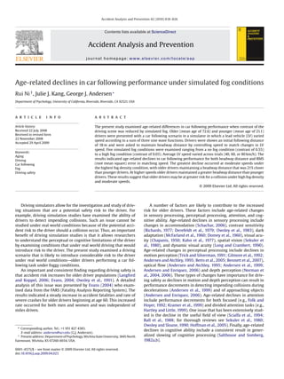
- 3. 820 R. Ni et al. / Accident Analysis and Prevention 42 (2010) 818–826 the response lag to changes in LV speed at a particular frequency. Squared coherence is a measure of squared correlation between the input and response at a particular frequency and provides a mea- sure of the variance accounted for in tracking performance. Squared coherence is defined as the ratio of the squared cross-amplitude values (of signal and response frequencies) to the product of the spectrum density estimates (of signal and response frequencies). These measures assessed performance changes based on dis- tance information and speed information. Specifically, mean and variance of distance headway are based on distance perception whereas RMS speed error, gain, phase angle, and squared coherence are based on speed perception. If the age and distance perception hypothesis is correct, then we expect age-related declines in mea- sures based on distance perception. If the age and speed perception hypothesis is correct, then we expect age-related declines in mea- sures based on speed perception. In addition, if older drivers have greater difficulty in detecting and responding to speed changes then we predict age-related declines will be greater as the overall speed of the LV is increased. Fig. 1. Sample image of the driving simulation scene. The fog density level depicted An important issue in car following is how to quantify a safe is an intermediate (0.08) level. following distance. Time headway (THW) is a measure used to assess safe car following performance and is derived by the ratio of to-normal vision and were currently licensed drivers. All drivers headway distance and velocity of the driver vehicle. This measure had experience driving in fog and reported driving at least 3 days indicates the time between two vehicles passing the same point per week. traveling in the same direction and is used as an indication of a safe margin between the driver and lead vehicle. In the present study we 1.2. Design required drivers to maintain a fixed distance of 18 m across the three speed conditions. Thus, THW would vary as a function of speed. Four independent variables were examined: Age (younger and This analysis allows one to determine changes in safe driving per- older drivers), simulated fog (simulated fog density of 0.0, 0.04, formance as a function of fog density. For example, consider car 0.08, 0.12, and 0.16), average LV speed (40 km/h, 60 km/h, and following at a specific constant speed. If drivers have difficulty in 80 km/h), and frequency of speed change (0.033, 0.083, 0.117 Hz). maintaining a safe margin as a function of fog then increased fog Age was run as a between subjects variable. All other variables were density should result in a decrease in THW. If older drivers have run as within subjects variables. greater difficulty than younger drivers under foggy conditions in determining distance and speed then they may follow at a closer distance resulting in a decrease in THW—an indication of increased 1.2.1. Apparatus crash risk. The displays were presented on Dell 670 Workstation. A Logitech Wingman Formula GP system, including acceleration and brake pedals, was used for closed loop control of the simulator. The dis- 1. Experiment plays were presented on a 35◦ × 47◦ visual angle monitor. Viewing distance was 60 cm. The display update was 60 Hz. 1.1. Drivers Eight college students (age mean and standard deviation of 21.0 1.2.2. Driving simulation scenario and 2.6, respectively) and eight older subjects (age mean and stan- The roadway consisted of three traffic lanes (representing a 3 dard deviation of 72.6 and 4.6, respectively) were recruited for the lane one way road) with the driver and LV located in the center study and were paid for their participation. Prior to the experi- lane (see Fig. 1). The LV was a white colored sedan (6.3 deg visual ment, all drivers were screened using visual and cognitive tests angle at a headway distance of 18 m). We used a white colored including Snellen static acuity, contrast sensitivity, WAIS-KBIT, and vehicle because of all vehicle colors it should be the most diffi- perceptual encoding (see Table 1). All reported normal or corrected- cult to see under foggy conditions. The Michaelson contrast of the rear tires and vehicle body, under the 0.0 fog density condition, was 0.55. Average luminance (measured using a Photo Research Table 1 PR-524 LiteMateTM photometer and based on luminance measures Means and standard deviations of participants’ demographic information and results from perceptual and cognitive tests. of 20 random locations in the display) of the driving scene was 24.7 cd/m2 . A black and white gravel texture pattern was used Variable Younger Older to simulate asphalt. Dashed lines (2 m in length positioned every M SD M SD 2 m along the roadway) were used to simulate lane markers. The Age (years)a 21.1 2.67 72.6 4.62 city buildings and LV were produced by digitally photographing Years of educationa 14.0 1.3 16.8 2.1 real buildings and vehicle and using the digital images as texture Snellen Letter Acuity 10/10.8 1.7 10/13 2.3 maps for the roadway scenes. The images were digitally altered to Log Contrast Sensitivitya , b 1.75 0.06 1.62 0.19 increase the realism of the simulator scene (e.g., remove specular Digit Span Forward 11.0 1.7 12.1 2.0 highlights, add shading) and were scaled to be appropriate with the Digit Span Backward 7.6 2.9 8.0 2.1 Perceptual Encoding Manuala 92.2 13.3 67.0 12.5 geometry of the simulation. Lane width was 3.8 m. Kaufman Brief Intelligence Test 28.3 4.4 29.9 4.8 Drivers were presented with a car following scenario in which a Differences between age groups were significant (p ≤ .05) for both sets of age the LV varied its speed according to a sum of 3 equal-energy sinu- groups. soids (i.e. the peak accelerations and decelerations of each sine b Contrast sensitivity was measured using the Pelli Robson test (Pelli et al., 1988). wave in the signal were equivalent). The corresponding amplitudes
- 4. R. Ni et al. / Accident Analysis and Prevention 42 (2010) 818–826 821 for these sinusoids were: 9.722, 3.889, and 2.778 km/h. The range to become familiar with the control dynamics of the simulator. Fol- of speeds produced by the sum of sines function was ±12.3 km/h lowing the practice session drivers were given two trials of each about the mean speed. At the beginning of each trial run, drivers combination of speed and fog density for a total of 30 trials. Trial were given 10 s of driving at a constant speed 18 m behind the duration was 1 min. Drivers were given a brief break following 15 constant speed LV to establish a perception of the desired dis- trials. The duration of the experimental session was 1 h. tance to be maintained. The three sinusoids were out of phase Feedback for the car following task was used by activating a with one another. The initial phase of the high and middle fre- horn sound if the headway (distance between the driver and LV) quency was selected randomly with the phase value of the low exceeded 24 m. The purpose of the horn was to ensure that the frequency selected to produce a sum of zero. This manipulation driver closely attended the car following task, and was intended to ensured that the speed profile of the LV, following the 5 s of con- simulate an impatient driver behind the driver’s vehicle. The horn stant speed, would vary from trial to trial with a smooth speed sound was used as feedback for both practice and experimental transition following the period of constant speed. trials. 1.2.3. Simulated fog 2. Results To simulate realistic effects of fog the computer simulation used the formula Two types of performance were assessed. Global driving perfor- mance was determined by deriving measures of mean following L(s, Â) = Lo Fex (s) + Lin (S, Â), (1) distance, variance of following distance, and RMS (root mean squared) speed error (driver speed relative to LV speed). Local per- where Lo represents the light reflected from the object, Fex (s) is the formance measures were determined by analyzing the speed of the amount of light that reaches the driver divided by the amount of driver’s vehicle using a fast Fourier transform (FFT) and deriving light decay that occurs with distance (Fex (s) can be replaced with control gain (output/input), phase angle, and squared coherence e−bms to represent the decay factor for fog using a Mei-scattering values for each frequency. criterion), and Lin (S, Â) represents the scattering of light from fog. This function is the industry standard for simulating fog in com- puter graphics and visualization (Klassen, 1987; Nishita, 1998; 2.1. Mean distance headway Hoffman and Preetham, 2003) and produces a contrast gradient that varies exponentially as a function of distance. The specific fog The mean distance headway (distance between driver and lead values in the simulation, using this equation, were 0.0, 0.04, 0.08, vehicle in meters) was calculated for each driver in each con- 0.12, and 0.16. These values were selected to represent a range of dition and analyzed in a 2 (age) × 5 (fog density) × 3 (speed) conditions from high visibility (0.0 fog condition) to low visibil- ANOVA. The main effect of fog on distance headway was signifi- ity (0.16 fog condition). The low visibility condition was selected cant, F(4,56) = 5.53, p < .05. The mean distance headway for the 0.0, based on informal observations indicating that under this condi- 0.04, 0.08, 0.12, and 0.16 simulated fog density levels were 19.3, 20.1, tion the visibility of the LV was considerably reduced at the desired 19.3, 18.2, and 17.9 m, respectively. Post hoc tests (Tukey HSD test) following distance of 18 m. indicated significant differences (p < .05) between the 0.04 and 0.12, To provide metrics that can be used to replicate the same and between the 0.04 and 0.16 fog density conditions. simulated fog conditions we calculated the variation in con- The main effect of speed was significant, F(2,28) = 17.4, p < .05. trast as a function of fog density. Contrast was determined by Mean distance headway for the 40, 60, and 80 km/h speeds were measuring luminance differences between the rear tire of the 17.7, 19.2, and 20.0 m, respectively. Post hoc tests indicted signifi- LV (the darkest region of the view of the LV) and the bumper cant differences between the 40 and 60 km/h, and between the 40 of the LV (the lightest region of the view of the LV). The mea- and 80 km/h speed conditions. The interaction between age group surements were taken with the LV at a simulated distance of and fog was significant, F(4,56) = 2.91, p < .05, and is shown in Fig. 2. 18 meters (the desired following distance). Contrast values According to this result, older drivers maintained a slightly greater were derived using the Michaelson contrast formula: Contrast headway distance for the no fog (0.0 fog density) condition. How- = (luminancemax − luminancemin )/(luminancemax + luminancemin ). ever, at higher fog density levels older drivers maintained a closer The contrast values for the 0.0, 0.04, 0.08, 0.12, and 0.16 simulated headway distance than younger drivers. fog density levels were 0.55, 0.25, 0.12, 0.06, and 0.03. The LV was visible to all drivers under the simulated fog conditions at the predetermined driving distance. 1.2.3.1. Procedure. Drivers were seated in the simulator and instructed to maintain their initial separation from the LV despite changes in speed of the LV. Each trial consisted of two phases. During the first phase (which lasted 5 s) the driver’s vehicle was positioned 18 meters behind the LV with a speed that matched the LV speed (40, 60, or 80 km/h). Control input (acceler- ation/deceleration) was not allowed during this phase and drivers were instructed that the headway distance during this phase was the desired headway distance. Following the first phase a tone sounded indicating the start of the second phase of the trial. During this phase control input was allowed and LV speed varied accord- ing to the sum of sine wave functions. Drivers were instructed that the LV speed would change and to maintain the following distance indicated during the first phase by using the acceleration and brake pedals. Drivers were given 15 min of practice in the simulator with changes in LV speed (determined by a single sine wave of 0.033 Hz) Fig. 2. Mean headway distance as a function of age of drivers and fog density.
- 5. 822 R. Ni et al. / Accident Analysis and Prevention 42 (2010) 818–826 Fig. 3. Mean headway distance as a function of age of drivers, fog density, and speed. The interaction between speed and fog density was significant 2.4. Speed measure: FFT analyses (F(8,112) = 2.58, p < .05) as well as the interaction of age, speed and fog density (F(8,112) = 3.09, p < .05; see Fig. 3). According to this The speed of the driver’s vehicle was recorded and analyzed result, older drivers consistently maintained a closer following dis- using a fast Fourier transform (FFT) with control gain (out- tance than younger drivers as a result of increased fog density put/input), phase angle, and squared coherence (the squared and increased speed. The largest age-related difference in distance correlation between the input and response at a particular fre- headway occurred at the intermediate speed (60 km/h) and high- quency) values derived for each frequency. The average gain, phase est fog density condition. However, a notable exception was the angle and squared coherence scores were derived for each driver highest fog density condition and highest speed. For this condition and analyzed in a 2 (age) × 3 (speed) × 3 (frequency) × 5 (fog den- older drivers had a greater following distance than younger drivers. sity) ANOVA. This result is likely due to a change in strategy employed by older drivers. Specifically, older drivers increased following distance at 2.5. Control gain high speeds to minimize the likelihood of a collision because of dif- ficulty in perceiving changes in the visual angle of the LV due to The results for control gain are shown in Fig. 4. The main effect of reduced contrast. speed was significant, F(2,28) = 25.2, p < .05. The average gain for the 40, 60, and 80 km/h speeds were 0.87, 0.93, and 0.95, respectively. 2.2. Headway distance variance Post hoc comparisons indicated significant differences between the 40 and 60 km/h speeds, and between the 40 and 80 km/h speeds. The variance of distance headway (distance between driver The main effect of fog was significant, F(4,56) = 3.1, p < .05. The aver- and lead vehicle) was calculated for each driver in each condi- age control gain for the 0.0, 0.04, 0.08, 0.12, and 0.16 fog density tion and analyzed in a 2 (age) × 5 (fog density) × 3 (speed) ANOVA. conditions were 0.93, 0.92, 0.92, 0.91, and 0.90, respectively. Post The main effect of age was significant (F(1,14) = 4.9, p < .05). This hoc comparisons indicated significant differences the 0.0 and 0.16 result indicated that older drivers had greater headway variance fog density conditions. The main effect of frequency was signifi- (mean variance of 25.6) compared to younger drivers (mean vari- cant, F(2,28) = 73.8, p < .05. The average gain for the 0.033, 0.083, ance of 10.1). There were no other significant main effects or 0.117 Hz frequencies were 0.99, 0.91, and 0.85, respectively. Post hoc interactions. comparisons indicated significant differences between all pairwise comparisons. Finally, the two way interaction between speed and 2.3. RMS speed error frequency was significant, F(4,56) = 27.9, p < .05. According to this result, the decrease in control gain with an increase in speed was The RMS speed error was derived for each driver in each most pronounced for the 0.117 frequency as compared to the 0.083 fog and speed condition and analyzed in a 2 (age) × 5 (fog den- and 0.033 Hz frequencies. sity) × 3 (speed) ANOVA. There was a significant main effect of There were no other significant main effects or interactions. age (F(1,14) = 5.8, p < .05) indicating greater RMS error for older drivers (mean RMS error of 6.17 km/h) as compared to younger 2.6. Control phase angle drivers (mean RMS error of 4.83 km/h). There was also a main effect of fog (F(4,56) = 3.2, p < .05). The mean RMS error for the 0.0, The results for control phase angle are shown in Fig. 4. The main 0.04, 0.08, 0.12, and 0.16 fog density levels were 5.17, 5.55, 5.29, effect of speed (F(2,28) = 28.3), fog density (F(4,56) = 4.03), and fre- 5.50, and 5.98 km/h, respectively. Post hoc analyses indicated a quency (F(2,28) = 55.5) were significant (p < .05). In addition, the significant difference between the 0.0 and 0.16 fog density condi- two way interactions between speed and fog (F(8,112) = 2.3), speed tions. There were no other significant main effects or interactions and frequency (F(4,56) = 8.9), and fog and frequency (F(8,112) = 2.78) (p > .05). were significant (p < .05). These results are consistent with the
- 6. R. Ni et al. / Accident Analysis and Prevention 42 (2010) 818–826 823 Fig. 4. Bode plot (control gain and phase angle) as a function of driver age group and fog density. results reported in Kang et al. (2008). There was no significant effect of the average speed of the LV with THW decreasing at increased of age nor did age interact with any other variables (p > .05). average speed of the LV. Thus, we conducted separate 2 (age) × 5 (fog density) for each speed condition. The results for THW are pre- 2.7. Squared coherence sented in Fig. 6. At the slowest speed (40 km/h) the main effect of fog was significant, F(4,56) = 4.83, p < .05. According to this result The results for squared coherence are shown in Fig. 5. The THW decreased as a function of fog density. The main effect of age main effect of age was significant, F(1,14) = 4.5, p < .05. The aver- [F(1,14) < 1] and the interaction of age and fog density [F(4,56) = 1.6] age squared coherence for the older and younger drivers were were not significant, p > .05. These results indicate that at the 0.89 and 0.94, respectively. The main effect of fog was significant, lowest average LV speed we did not find any significant differ- F(4,56) = 4.6, p < .05. The average squared coherence for the 0.0, 0.04, ences in car following performance between older and younger 0.08, 0.12, and 0.16 fog density conditions were 0.92, 0.91, 0.92, 0.91, drivers. and 0.90, respectively. Post hoc comparisons indicated significant At the intermediate speed (60 km/h) the main effect of fog den- differences between 0.0 and 0.16 fog density conditions. This result sity was significant, F(4,56) = 18.5, p < .01 as well as the interaction indicates decreased car following performance under the highest between driver age and fog density, F(4,56) = 5.75, p < .01. According fog density condition examined. There were no significant interac- to this result, THW decreased for both older and younger drivers tions between age and the other variables, p > .05. with an increase in fog density. However, older drivers had the 2.8. Time headway largest decrease in THW at the highest fog condition. This result indicates that older drivers, as compared to younger drivers, had a To examine the effects of fog on the safety margin for car follow- significant reduction in the safety margin at the highest fog density ing we derived time headway (THW) data. THW varied as a function level.
- 7. 824 R. Ni et al. / Accident Analysis and Prevention 42 (2010) 818–826 Fig. 5. Mean Squared coherence as a function of driver age group, frequency, and fog density. At the highest speed (80 km/h) the main effect of fog density was conditions. According to the aging and distance perception hypoth- significant, F(4,56) = 2.73, p < .05 as well as the interaction between esis, older drivers, as compared to younger drivers, will have driver age and fog density, F(4,56) = 3.12, p < .05. According to this decrements in perceived distance to the LV. According to the result older and younger drivers had a decrease in THW with an aging and speed perception hypothesis, older drivers, as com- increase in fog density with the exception of the highest fog den- pared to younger drivers, will have decrements in perceived speed sity condition. For younger drivers THW continued to decrease at and relative speed change between the lead and following vehi- the highest fog density condition. However, for older drivers THW cle. The results of the present study provide evidence in support increased at the highest fog density condition. This result suggests of both of these hypotheses. With regard to distance informa- that older drivers increased the following distance to increase the tion, we found that older drivers, as compared to younger drivers, safety margin. followed at a closer headway distance with an increase in fog den- sity. In addition, although mean headway distance varied for both 3. General discussion younger and older drivers as a function of speed, older drivers showed a greater change as a result of speed. This effect was The present study examined two hypotheses concerning age- especially pronounced for the highest fog density conditions exam- related differences in car following performance under foggy ined. We also found greater variance in distance headway for older Fig. 6. Safety martin (time headway) as a function of driver age group, fog density and speed.
- 8. R. Ni et al. / Accident Analysis and Prevention 42 (2010) 818–826 825 drivers, as compared to younger drivers. These results provide Acknowledgement evidence in support of the age and distance perception hypothe- sis. This research was supported by NIH grant AG13419-06 and NIH With regard to speed perception the results indicated that EY18334-01. older drivers had greater RMS speed error than younger drivers. In addition, older drivers had lower squared coherence scores than younger drivers, indicating that older drivers had poorer perfor- References mance in tracking local variations in speed at specific frequencies of LV speed. These results provide evidence in support of the age Andersen, G.J., Atchley, P., 1995. Age-related differences in the detection of three- dimensional surfaces from optic flow. Psychology and Aging 10, 650–658. and speed perception hypothesis. The results of the present study, Andersen, G.J., Braunstein, M.L., 1998. The perception of depth and slant from texture considered together, suggest that older drivers have decreased car in 3D scenes. Perception 27, 1087–1106. following performance as a result of difficulty in judging both speed Andersen, G.J., Cisneros, J., Atchley, P., Saidpour, A., 1999. Speed, size, and edge- rate information for the detection of collision events. Journal of Experimental and distance. Psychology. Human Perception and Performance 25, 256–269. An important finding in the present study was the interaction Andersen, G.J., Enriquez, A., 2006. Aging and the detection of observer and moving of age, speed, and fog density for the distance headway measure. object collisions. Psychology and Aging 21, 74–85. Of particular interest were the age-related performance differences Andersen, G.J., Sauer, C.W., 2004. Optical information for collision detection dur- ing deceleration. In: Hecht, H., Kaiser, M. (Eds.), Theories of Time to Contact: for the 60 km/h speed condition under the highest fog density con- Advances in Psychology Series. Elsevier/North Holland, Amsterdam, Nether- dition (see Figs. 3 and 6). Under this condition older drivers, as lands, pp. 93–108. compared to younger drivers, followed at a very close distance and Andersen, G.J., Sauer, C.W., 2005. Visual information for car following by drivers: the role of scene information. Transportation Research Record F 1899, 104–109. shorter THW. We believe older drivers followed at a close distance Andersen, G.J., Sauer, C.W., 2007. Optical information for car following: the driving because of reduced visibility due to fog and the increased diffi- by visual angle (DVA) model. Human Factors 49, 878–896. culty to perceive changes in LV speed. This combination of speed Ball, K., Beard, B.L., Roenker, D.L., Miller, R.L., Griggs, D.S., 1988. Age and visual search: Expanding the useful field of view. Journal of the Optical Society of America, A, and fog density resulted in the greatest difference in performance Optics, Image & Science 5, 2210–2219. between younger and older drivers and suggests a serious colli- Bennett, P.J., Sekuler, R., Sekuler, A.B., 2007. The effects of aging on motion detection sion risk for older drivers. We can assess collision risk by deriving and direction identification. Vision Research 47, 799–809. Betts, L.R., Taylor, C.P., Sekuler, A.B., Bennett, P.J., 2005. Aging reduces center- the time gap (the amount of time to close the following distance). surround antagonism in visual motion processing. Neuron 45, 361–366. The shorter the time gap the less time available to the driver Bian, Z., Andersen, G.J., 2008. Aging and the perceptual organization of 3-D scenes. to avoid a collision. For the 60 km/h/0.16 fog density condition Psychology and Aging 23, 342–352. Brackstone, M., McDonald, M., 1999. Car-following: a historical review. Transporta- younger drivers had an average time gap of 1.1 s. However older tion Research Record F 2, 181–196. drivers had a time gap of 0.87 s. This represents a 21% reduction Broughton, K.L.M., Switzer, F., Scott, D., 2007. Car following decisions under three in time available to respond to avoid a collision for older drivers. visibility conditions and two speeds tested with a driving simulator. Accident Given the well documented finding of slower reaction time with Analysis & Prevention 39, 106–116. Chandler, R.E., Herman, R., Montroll, E.W., 1958. Traffic dynamics: studies in car age this result suggests that older drivers may be at considerable following. Operations Research 6, 165–184. risk of a collision under high fog density conditions at moderate Chapanis, A., 1950. Relationships between age, visual acuity and color vision. Human speeds. Biology 22, 1–33. Derefeldt, G., Lennerstrand, G., Lundh, B., 1979. Age variations in normal human An interesting change in the pattern of results occurred for older contrast sensitivity. Acta Ophthalmologica 57, 679–690. drivers at the 80 km/h speed. At this speed under the highest fog Domey, R.G., McFarland, R.A., Chadwick, E., 1960. Dark adaptation as a function of density condition examined older drivers maintained a following age and time. II: A derivation. Journal of Gerontology 15, 267–279. Evans, L., 2004. Traffic Safety. Science Serving Society, Bloomfield Hills, MI, p. 179. distance and THW that was much greater than the following dis- Folk, C.L., Hoyer, W.J., 1992. Aging and shifts of visual spatial attention. Psychology tance of younger drivers (see Figs. 3 and 6). Unlike the results for the and Aging 7, 453–465. 60 km/h speed (which we believe is due to perceptual difficulty for Gilmore, G.C., Wenk, H.E., Naylor, L.A., Stuve, T.A., 1992. Motion perception and aging. Psychology and Aging 7, 654–660. older drivers) we believe the results for the 80 km/h speed are due to Hartley, A.A., Little, D.M., 1999. Age-related differences and similarities in dual-task a combination of perceptual difficulty and a strategic shift by older interference. Journal of Experimental Psychology 128, 416–449. drivers. Specifically, older drivers may be aware of the difficulty in Helly, W., 1959. Simulation of bottlenecks in single lane traffic flow. In: Proceedings of the Symposium on Theory of Traffic Flow, Research Laboratories, General Motors. perceiving changes in LV speed under the high fog condition and, Elsevier, New York, pp. 207–238. because of the decreased THW, adopt a greater following distance Hoffman, L., McDowd, J.M., Atchely, P., Dubinsky, R., 2005. The role of visual atten- to increase the safety margin. tion in predicting driving impairment in older adults. Psychology and Aging 20, These results of the preset study suggest two human factors 610–622. Hoffman, N., Preetham, A.J., 2003. Real-time light-atmosphere interactions for out- applications. The first application concerns car following mod- door scenes. In: Lander, J. (Ed.), Graphics Programming Methods. Charles River els. As noted earlier, the DVA model (Andersen and Sauer, 2007) Media, Rockland, MA, pp. 337–352. includes components for distance headway and speed. A modifi- Jagacinski, R.J., Flach, J.M., 2003. Control Theory for Humans: Quantitative Approaches to Modeling Performance. Erlbaum, Mahway, NJ. cation of the DVA model to account for car following under fog Kahn, H.A., Leibowitz, H.M., Ganley, J.P., Kini, M.M., Colton, T., Nickerson, R.S., et conditions should focus on changes in both the distance and speed al., 1977. The Framingham Eye Study. I. Outline and major prevalence findings. components. For example, adding a noise parameter for estimating American Journal of Epidemiology 106, 17–32. Kang, J.J., Ni, R., Andersen, G.J., 2008. The effects of reduced visibility from fog on car distance and speed change may allow the model to predict car fol- following performance. Transportation Research Record: Journal of the Trans- lowing performance under fog conditions. Age-related differences portation Research Board 2069, 9–15. in car following performance can be incorporated in the model by Klassen, R.V., 1987. Modeling the effect of the atmosphere on light. ACM Transactions on Graphics (TOG) 6 (3), 215–237. using a greater magnitude of noise for the distance component. A Kramer, A.F., Hahn, S., Irwin, D.E., Theeuwes, J., 1999. Attentional capture and aging: second application concerns in-vehicle warning systems or adap- Implications for visual search performance and oculomotor control. Psychology tive control systems for reduced visibility conditions. The results of and aging 14, 135–154. Langford, J., Koppel, S., 2006. Epidemiology of older driver crashes—Identifying older the present study indicate that older drivers have greater difficulty, driver risk factors and exposure patterns. Transportation Research. Part F, Traffic under fog conditions, in maintaining distance headway. This find- Psychology and Behaviour 9, 309–321. ing suggests that the development of warning systems or adaptive Larish, J.F., Flach, J.M., 1990. Sources of information useful for perception of speed control systems to improve driver safety, particularly for reduced of rectilinear motion. Journal of Experimental Psychology: Human Perception & Performance 16, 295–302. visibility conditions, should focus on distance headway information Long, G.M., Crambert, R.F., 1990. The nature and basis of age-related changes in in minimizing collision risk. dynamic visual acuity. Psychology and Aging 5, 138–143.
- 9. 826 R. Ni et al. / Accident Analysis and Prevention 42 (2010) 818–826 Massie, D.L., Campbell, K.L., Williams, A.F., 1995. Traffic accident involvement rates Richards, O.W., 1977. Effects of luminance and contrast on visual acuity, ages 16 by driver age and gender. Accident Analysis & Prevention 27, 73–87. to 90 years. American Journal of Optometry and Physiological Optics 54, 178– McFarland, R.A., Domey, R.G., Warren, A.B., Ward, D.C., 1960. Dark adaptation as a 184. function of age: I. A statistical analysis. Journal of Gerontology 15, 149–154. Salthouse, T.A., Somberg, B.L., 1982a. Time–accuracy relationships in young and old McGwin, G., Brown, D.B., 1999. Characteristics of traffic crashes among young, adults. Journal of Gerontology 37, 49–53. middle-aged and older drivers. Accident Analysis & Prevention 31, 181–198. Salthouse, T.A., Somberg, B.L., 1982b. Isolating the age deficit in speeded perfor- Nishita, T., 1998. Light scattering models for the realistic rendering of natural scenes. mance. Journal of Gerontology 37, 59–63. In: Rendering Techniques ‘98, Proceedings of the Eurographics Rendering Work- Schachar, R.A., 2006. Effect of change in central lens thickness and lens shape on age- shop, pp. p1–10. related decline in accommodation. Journal of Cataract and Refractive Surgery 32, Norman, F.J., Clayton, A.M., Shular, C.F., Thompson, S.R., 2004. Aging and the per- 1897–1898. ception of depth and shape from motion parallax. Psychology and Aging 19, Schiff, W., Oldak, R., Shah, V., 1992. Aging persons’ estimates of vehicular motion. 506–514. Psychology & Aging 7 (4), 518–525. Norman, F.J., Crabtree, C.E., Hermann, D., 2006. Aging and the perception of 3-D Scialfa, C.T., Guzy, L.T., Leibowitz, H.W., Garvey, P.M., et al., 1991. Age differences in shape from kinetic patterns of binocular disparity. Perception & Psychophysics estimating vehicle velocity. Psychology & Aging 6 (1), 60–66. 68, 94–101. Scialfa, C.T., Thomas, D.M., Joffe, K.M., 1994. Age differences in the useful field Owsley, C., Ball, K., Sloane, M.E., Roenker, D.L., Bruni, J.R., 1991. Visual/cognitive cor- of view: An eye movement analysis. Optometry and Vision Science 71, 736– relates of vehicle accidents in older drivers. Psychology and Aging 6, 403–415. 742. Owsley, C., Sekuer, R., Siemsen, D., 1983. Constrast sensitivity throughout adulthood. Sekuler, R., Hutman, L.P., Owsley, C.J., 1980. Human aging and spatial vision. Science Vision Research 23, 689–699. 209, 1255–1256. Owsley, C., Sloane, M.E., 1990. Vision and Aging. In: Nebes, R.D., Corkin, S. (Eds.), Stutts, J.C., Martell, C., 1992. Older driver population and crash involvement trends Handbook of Neuropsychology, vol. 4. Elsevier Science, New York, NY, pp. 1974–1988. Accident Analysis & Prevention 24, 317–327. 229–249. Trick, G.L., Silverman, S.E., 1991. Visual sensitivity to motion: Age-related changes Pelli, D.G., Robson, J.G., Wilkins, A.J., 1988. Designing a new letter chart for measuring and deficits in senile dementia of the Alzheimer type. Neurology 41, 1437– contrast sensitivity. Clinical Visual Neuroscience 2, 187–199. 1440.