dx

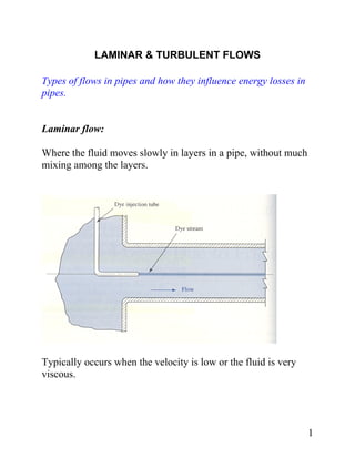
1. LAMINAR & TURBULENT FLOWS
Types of flows in pipes and how they influence energy losses in
pipes.
Laminar flow:
Where the fluid moves slowly in layers in a pipe, without much
mixing among the layers.
Typically occurs when the velocity is low or the fluid is very
viscous.
1

2. 2

3. Turbulent flow
Opposite of laminar, where considerable mixing occurs,
velocities are high.
Laminar and Turbulent flows can be characterized and
quantified using Reynolds Number
established by Osborne Reynolds
and is given as –
3

4. V Dρ VD
NR = =
η ν
Where NR – Reynolds number
V – velocity of flow (m/s)
D – diameter of pipe (m)
ρ – density of water (kg/m3)
ή – dynamic viscosity (kg/m.s)
ν – kinematic viscosity (m2/s)
when – units are considered – NR is dimensionless.
NOTE – Reynolds number directly proportional to velocity
& inversely proportional to viscosity!
NR < 2000 – laminar flow
NR > 4000 – Turbulent flow
4

5. For 2000 < NR < 4000 – transition region or critical region –
flow can either be laminar of turbulent – difficult to pin down
exactly.
More viscous fluid will tend to have laminar flow or lower
Reynolds number.
Reynolds numbers for some real-life examples –
• Blood flow in brain ~ 100
• Blood flow in aorta ~ 1000
• Typical pitch in major league baseball ~ 200000
• Blue whale swimming ~ 300000000
5

6. Problem 8.1:
Determine the Reynolds number for –
Glycerin at 25C
Pipe at D = 150 mm = 0.15 m
Velocity = V = 3.6 m/s
ρ = 1258 kg/m3
ή = 0.96 Pa.s or (kg/m.s)
V Dρ
NR =
η
= 3.6 * 0.15 * 1258 / 0.96 = 708
Nr < 2000; therefore flow is laminar!
6

7. Friction losses in Pipes
Vary with laminar or turbulent flow
Energy equation can be given as –
p1/γ + z1 + v12/2g + hA – hR – hL = p2/γ + z2 + v22/2g
where hA, hR, hL are the heads associated with addition,
removal and friction loss in pipes, respectively.
note that the terms are added on the LHS of the equation!
The head loss in pipes = hL can be expressed as –
hL = f * (L/D) * v2/2g
- Darcy’s equation for energy loss (GENERAL FORM)
Where
f – friction factor
L – length of pipe
D – diameter of pipe
v – velocity of flow
How do these factors affect losses???????????
7

8. Similarly,
Another equation was developed to compute hL under Laminar
flow conditions only
32 η L V
hL =
γ D2
- called the Hagen-Poiseuille equation
If you equate Darcy’s equation and Hagen-Poiseuille equation
Then we can find the friction factor f
64η 64
f = =
V D ρ NR
Thus the friction factor is a function of Reynold’s number!
8

9. Example Problem 8.4
Determine energy loss if –
Glycerin at 25C
L = 30m
D = 150 mm = 0.15 m
V = 4.0 m/s
Density = 1258 k/m3
Dynamic viscosity = 0.96 Pa.s
First determine the Reynolds number to determine if it is
laminar flow
V Dρ
NR =
η
= 4.0 * 0.15 * 1258 / 0.96 = 786 < 2000 - Laminar flow
Therefore Darcy’s equation
hL = f * (L/D) * (v2/2g)
= 64/NR * (L/D) * (v2/2g)
= 13.2 m
9

10. Friction losses for Turbulent Flow
For Laminar flow we got a nice equation to compute the friction
factor – dependent ONLY on Reynolds number!
In case of Turbulent flow – friction factor computed based
on inside roughness of the pipe and Reynolds number!
Roughness is expressed as - Relative roughness = D/ε
(not the best way to express it!)
• More rough pipe – low D/ε
• Less rough pipe – high D/ε
Friction factor for Turbulent flow ~ Relative roughness &
Reynolds number
Roughness values for various pipes – Table 8.2
10

11. Some Roughness values from Table 8.2
Material Roughness ε (m)
Plastic 3.0 x 10-7
Steel 4.6 x 10-5
Galvanized iron 1.5 x 10-4
Concrete 1.2 x 10-4
Question - **Why doesn’t ε affect loss in laminar flow
conditions ?????????
11

12. The Moody Diagram
Developed to provide the friction factor for turbulent flow for
various values of Relative roughness and Reynold’s number!
Curves generated by experimental data.
12

13. Key points about the Moody Diagram –
1. In the laminar zone – f decreases as Nr increases!
2. f = 64/Nr.
3. transition zone – uncertainty – not possible to predict -
4. Beyond 4000, for a given Nr, as the relative roughness term
D/ε increases (less rough), friction factor decreases
5. For given relative roughness, friction factor decreases with
increasing Reynolds number till the zone of complete
turbulence
6. Within the zone of complete turbulence – Reynolds number
has no affect.
7. As relative roughness increases (less rough) – the boundary
of the zone of complete turbulence shifts (increases)
If you know the – relative roughness, Reynolds number –
you can compute the friction factor from the Moody
Diagram
13

14. 14

15. Swamee and Jain converted the graph into an equation!
For the turbulent portion -
(less than 1% error)
0.25
f = 2
⎡ ⎛ 1 ⎞ 5.74 ⎤
⎢ log ⎜
⎜ 3.7 ( D / ε ) ⎟ + N 0.9 ⎥
⎟
⎢ ⎝
⎣ ⎠ R ⎥ ⎦
15

16. Example problem 8.5:
Determine friction factor if water at 160 F is flowing at 30
ft/s in an uncoated ductile iron pipe having an inside
diameter of 1.0 inch.
Determine Reynolds number:
V Dρ VD
NR = =
η ν
D = 1/12 = 0.0833 ft; V = 30 ft/s; ν = 4.38 x 10-6 ft2/s
NR = 5.70 x 105
So its turbulent flow, we will have to use Moody diagram
Determine relative roughness –
ε for ductile iron pipe from table 8.2 in text = 8 x 10-4 ft
D/ ε = 0.0833/8 x 10-4
= 104, use 100 for moody diagram
Using those values and going into Moody’s diagram, we get –
16

17. f = 0.0038.
17

18. Hazen-William formula
Alternate formula to compute head loss due to friction
Applicable for –
- Water
- D – larger than 2 inches and less than 6ft
- Velocity should not exceed 10 ft/s
The formula is unit-specific
For SI units –
1.852
⎡ Q ⎤
hL = L ⎢ ⎥
⎣ 0.85 A C h R 0.63 ⎦
Where
Q = 0.85 A C h R 0.63 s 0.54
Where R – hydraulic radius = area/perimeter of pipe.
Ch – Hazen Williams Coefficient
and s – slope gradient of the pipe.
18

19. Head Additions and Losses due to Pumps and Motors
(CHAPTER 7)
Bernoulli’s Energy equation can be given as –
p1/γ + z1 + v12/2g + hA – hR – hL = p2/γ + z2 + v22/2g
where hA, hR, hL are the heads associated with addition, removal
and friction loss in pipes, respectively.
also known as the GENERAL ENERGY EQUATION
represents the system in reality (not idealized conditions)
19

20. hA – head/energy additions due to pumps.
hR – head/energy removal due to motors.
hL – head losses due to friction and losses due to fittings, bends,
valves.
MAJOR LOSSES – motors, friction loss
MINOR LOSSES – valves, fittings, and bends
Typically
hL = K * v2/2g
that’s what we saw before with respect to Darcy’s Equation.
20

21. Example Problem 7.1: Finding TOTAL head loss due to
friction, valves, bends etc. –
Given –
Water moving in the system
Q = 1.20 ft3/s
Calculate TOTAL head loss due to valves, bends, and pipe
friction.
How should we proceed???????????
21

22. Apply the General Energy Equation for pts 1 and 2!
p1/γ + z1 + v12/2g - hL = p2/γ + z2 + v22/2g
cancel out the terms –
p1/γ + z1 + v12/2g - hL = p2/γ + z2 + v22/2g
and we get –
hL = (z1- z2) - v22/2g
(z1- z2) = 25 ft
How do we find v2???
Area of 3 inch dia pipe = 0.0491 ft2
v2 = 1.20 / 0.0491 = 24.4 ft/s
hL = 25 – (24.4)2/2*32.2 = 15.75 ft
22

23. Example Problem 7.2: - Now we will introduce a Pump and
determine the energy added by a pump!
• Q = 0.014 m3/s
• Fluid – Oil at Sg = 0.86; γ = 0.86 * 9.81 = 8.44 kN/m3
• hL = head loss due to friction, fittings, etc. = 1.86 Nm/N
Energy added by Pump????????????????????
23

24. Apply the General Energy Equation for pts. A and B!
pA/γ + zA + vA2/2g + hA - hL = pB/γ + zB + vB2/2g
Rearrange the equation!
hA = hL + (pB – pA) / γ + (zB – zA) + (vB2 - vA2 ) / 2g
(pB – pA) / γ = (296-(-28))/8.44 = 38.4 m
(zB – zA) = 1.0 m
How will you find velocities?????
Area at A = 0.004768 m2
Area at B = 0.002168 m2
vA = 2.94 m/s
vB = 6.46 m/s
plug all terms back in the original equation –
hA = hL + (pB – pA) / γ + (zB – zA) + (vB2 - vA2 ) / 2g
24

25. and hA = 1.86 + 38.4 + 1.0 + 1.69 = 42.9 m or 42.9 N.m/N
25

26. Power supplied by Pumps
Power of the pump = energy being transferred
PA = hA * W (where W is the weight flow rate)
= hA * γ *Q
SI units of power = watt (W) = 1.0 N.m/N or 1.0 Joule
US units of Power = lb-ft/s
1 horsepower = 1 hp = 550 lb-ft/s
1 hp = 745.7 Watt
Efficiency of the Pump
= (Power delivered to the fluid/ Power supplied to the pump)
= (PA/PI)
26

27. Example Problem 7.3: Determine the efficiency of the Pump
PI = 3.85 hp
Q = 500 gal/min of oil = 1.11 ft3/s
γ of oil = 56.0 lb/ft3
What is PA????
And what is efficiency (em) ????
So how do you proceed????????????????????
27

28. Apply the General Energy Equation for pts 1 and 2!
p1/γ + z1 + v12/2g + hA = p2/γ + z2 + v22/2g
Rearrange the equation!
hA = (p2 – p1) / γ + (z2 – z1) + (v22 - v12 ) / 2g
let’s solve for each term
γm = 13.54*62.4 = 844.9 lb/ft3
pressure difference using the manometer –
p1 + γo y + 20.4*γm – 20.4*γo - γo y = p2
(p2 – p1) / γo = (γm*20.4 / γo) – 20.4
= (844/56 -1) * 20.4 = 24.0 ft
Elevation difference is zero!
Find out the velocity head term???
28

29. A1 = 0.2006 ft2
A2 = 0.0884 ft2
V1 = 5.55 ft/s
V2 = 12.6 ft/s
(v22 - v12 ) / 2g = 1.99 ft
Substituting the terms –
hA = (p2 – p1) / γ + (z2 – z1) + (v22 - v12 ) / 2g
hA = 24.0 + 0 + 1.99 = 25.99 ft
PA = hA * γo *Q = 25.99 * 56.0 * 1.11 = 1620 lb-ft/s
= 1620/550 = 2.95 hp
em = 2.95/3.85 = 0.77
We have the answer!
29

30. Similarly, Power delivered to motors
PR = hR * γ *Q
Efficiency of the motor
= (Power output/ Power delivered by fluid)
= (PO/PR)
ASSIGNMENT # 6
1. 7.7M
2. 7.13M
3. 8.1E
4. 8.33E
30