1. Saito, R., M. lower ͑ Dresselhaus, is M. S. from Eq.
minus sign the Fujita, G. ͒ band. Itand clear Dresselhaus, ͑6͒
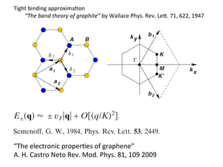
that Tight
bspectrum is Lett. 60, 2204. around zero energy if tЈ
lectronic propertiespproxima0on
the inding
a of graphene
1992a, Appl. Phys. symmetric
Saito,finite values graphite”
by
Wallace
Phys.
Rev.
Le<.
71,
622,
1947
is
= 0. For
“The
band
theory
of
R., M. Fujita, of tЈ, the electron-hole symmetry
G. Dresselhaus, and M. S. Dresselhaus,
broken and theRev.and 1804.
, 1992b, Phys.
B 46, * bands become 1asymmetric. In
San-Jose, P., E. Prada, and D. Golubev,k2007,bPhys. Rev. B 76,
-
Fig. 3, we show theAfullBband structure of graphene with y
195445.
,
both t and S.,. 2007, Phys. Rev.figure, we also show a zoom in
Saremi, tЈ δ 3 the1 same B 76, 184430.
In δ K
,
of the band D., E. H. Hwang, and W. K.ofΓ the Dirac points ͑at
Sarma, S. structure close to one Tse, 2007, Phys. Rev. B
s
the K or KЈ a 1
75, 121406. pointδ 2in the BZ͒. This dispersion can be M kx
c Schakel, A. M.2J., 1991, the full band structure, Eq. ͑6͒,
obtained by expanding Phys. Rev. D 43, 1428.
a
K’
t
close to the K ͑orGeim, vector, Eq. ͑3͒, as kE. H. + q, P.
Schedin, F., A. K. KЈ͒ S. V. Morozov, D. Jiang, = K Hill, with
b2
a Blake, and K. S. Novoselov, 2007, Nature Mater. 6, 652.
͉q ͉ Ӷ ͉K͉ ͑Wallace, 1947͒,
n Schomerus, H., 2007, Phys. Rev. B 76, 045433.
- Schroeder,͑ColorM. + O͓͑q/K͒2͔, and A. Javan, 1968, Phys. ͑7͒
FIG. 2. online͒ Honeycomb lattice and its Brillouin
E±͑q͒ Ϸ P. R., ͉q͉ S. Dresselhaus,
± vF
; zone.Lett. 20, 1292.structure of graphene, made out of two in-
Rev. Left: lattice
Semenoff, G. momentumRev. ͑a1 53, a2 are
where q is theW.,triangular latticesLett. and 2449. the latticethe
terpenetrating 1984, Phys. measured relatively to unit
- Sengupta, and ␦i G. 1 , 2the are the nearest-neighbor by vF
vectors, and
Dirac pointsK., and, viF=Baskaran, 2008, Phys. Rev. B given vectors͒.
is , 3 Fermi velocity, 77, 045417.
Seoanez, C., a value vandf
1raphene”
The This result are lo-
“The
electronic
proper0es
o A. H. Castro Neto, 2007, Phys.
F. Guinea, Ӎ g ϫ 106 m / s. Dirac cones was
Right: corresponding Brillouin zone.
= 3ta / 2,.
Castro
Neto
Rev.
Mod.
Phys.
81,
109
2009
- A.
H with 125427. KЈ F
catedB 76, K and
Rev. at the points.
first obtained by Wallace ͑1947͒.
-
2. form Left: energy spectrum ͑in units of t͒ for finite values of
lattice. ͑Wallace, 1947͒
t and tЈ, with t = 2.7 eV and tЈ = −0.2t. Right: zoom in of the
E±͑k͒ = ± tͱ3 + f͑k͒ − tЈf͑k͒,
energy bands close to one of the Dirac points.
1
f͑k͒ = 2 of tЈ is not 4 cos ͩ ͪ ͩ ͪ
ͱ3
ky cos kxa
3
The valuecos͑ͱ3kya͒ + well knownabut ab initio , calcula
͑6͒
͑Reich et al., 2002͒ find 0.02t Շ tЈ2 0.2t depending on the t
Շ 2
binding parametrization. These the upperet͑al.:alsoelectronic pro
where the plus sign applies to calculations*Theand the
Castro Neto
͒ include
effect of a third-nearest-neighbors hopping, which has a v
minus sign the lower ͑͒ band. It is clear from Eq. ͑6͒
of around 0.07 eV. A tight-binding fit to cyclotron reson
that the spectrum is symmetric around zero energy if tЈ
experiments ͑Deacon et al., 2007͒ finds tЈ Ϸ 0.1 eV.
= 0. For finite values of tЈ, the electron-hole symmetry is
broken and the and * bands become asymmetric. In
Fig. 3, we show the full band structure of graphene with
both t and tЈ. In the same figure, we also show a zoom in
of the band structure close to one of the Dirac points ͑at
the K or KЈ point in the BZ͒. This dispersion can be
3. anប = 1͒ ͚ e−ik·Rna͑k͒,
͑we use units such that = ͱN k
͑15͒
c
H=−t ͚is
by A = 3ͱ3a / 2.͗i,j͘,
2
It
†
͑a,ib,j + H.c.͒
where Nc is the number of unit cells.
c
tates for graphene is mation, we write the field an as a
. Dirac fermions
͚ † †
coming+ b,ib,j + H.c.͒, Fourier s
of carbon nanotubes ͑a,ia,j
− tЈ from expanding the
er shows 1 / ͱE singu- K. This produces an Јapproximation
͗͗i,j͘͘,
We consider the Hamiltonian ͑5͒ withas a sum of two ne
tion of the field an t = 0 and the
their electronic spec- the electron operators,
ourier transform of ͒ annihilates ͑creates͒ an electron
where the ͑ai, †
antization of ai, mo-
ular spin tube axis. ͒ on site Ӎ i −iK·RsublatticeЈ·Rna ͑an equ
to the ͑ = ↑ , ↓ an e
R on na + e−iK A ,
1,n 2,n
nanoribbons, whichis used for sublattice B͒, t͑Ϸ2.8 eV͒ i
lent definition
1
= ͚ e−ik·Rna͑k͒,
anearest-neighbor hopping energy ͑hopping between
ͱN c k
perpendicular to the
n ͑16͒
milar ferent sublattices͒, and t is the next −iKЈ·Rn
to carbon nano-
bn Ӎ e−iK·Rnb1,n + e nearest-neig
Ј b2,n ,
hopping energy1 ͑hopping in the same sublattice͒.
where Nc is the number of unit cells. Using this transfor-
energy bands derived from this Hamiltonian have
mation, we write the field an as a sum of two terms,
2009
form ͑Wallace, 1947͒
4. ͩ
͑ai bi ͒ ͱ = 1
† †
− ,3a͑i −͑i 3͒/4, 2͒.
y ͪͬ
guage,1 the two-component
It 0is clear that around K has the fo
mentum the effective Ham
ͫͩ ͪ ͬͪ
oniant ͵ dxdy⌿ is madeͱ of 3a͑1 − iͱclose to of ͱthe3a͑− i − ͱ3͒/4 /2 ⌿Di
two 3͒/4 + ץthe K massless ˆ ͑r͒ ͪ ͩ ͪͬ
point, obeys
ͩͪ ͬ ͪ
H Ӎ − ͑18͒3a͑i − ͱ3͒/4 copies 0
0
ˆ ͑r͒
0 †
−ik ץ
ץy holding for − 3͒/4 1 e K and
1 x y 1
− 3a͑1 + i 3͒/4 ˆ0
⌿2͑r͒ − 3a͑i 0
ke− Hamiltonian, 3a͑1 + iͱ3͒/4 one p around E
ͱ3͒/4
− i + ⌿ ͑r͒ˆ †
ther for p 3a͑1 − i ͫͩ 0 0
− around
2
−±,K͑k͒ ·=ٌ ͱ3͒/4
ͱ3͒/4 K0 . Note− 3a͑− i − ͱ3͒/4 first ץ
Ј + ץ
that, in 0 x ͩ
0ivF 3a͑i −͑r͒ =iˆ /2 ͑r͒.
ͱ2 quantized
±e⌿ k ͑r͒ y 2
The wave function, in m
= − i ͵ dxdy͓⌿ ͑r͒ · ٌ⌿ ͑r͒ + ⌿ ͑r͒ · ٌ⌿ ͑r͔͒,
uage,v the two-componentfor HK = vFwave where the
ˆ †ˆ ˆ ˆ electron · k, function
†
͑18͒
mentum around K has the
F 1 * 2
1 2
lose to the K point, obeyseigenenergies E = ± vFk, that the 2D Dirac equation,
− ivF · ٌ͑r͒ = E͑r͒. tion ±,Kthe = ͱ
respectively, and
with Pauli matrices = ͑ , ͒, = ͑ , − ͒, and ⌿
* ˆ
1 k −ikgiven
for 1 p 2 ±eik †
e is /2
͑k͒ momentum/2arou ͑ ͩ ͪ
ͩ ͪ
x y x y ˆ
h= · . i
= ͑a† , b†͒͑i = 1 , 2͒. It is clear that the effective Hamil-
The wave function, in momentum ͉p͉space, for/2the m
i i 2
e ik
1 where the
onian ͑18͒ is made of two copies of the massless Dirac-
for HK =͑k͒thek,
±,KЈ vF =· definition −i that the
ˆ = around· Kp Note that, in first quantized lan-
1
mentum around K has the formis clear from
ike Hamiltonian, one holding for p around K and the
ͱ
It ˆ
of h /2
other h p
for Ј. . ͑22͒ ˆk
±e
eigenenergies E = ± vof k, tha2
ͩ ͪ
2 ͉p͉
guage, the two-component electron wave function ͑r͒, and Ј͑r͒ are also eigenstates F h,
K
respectively, ͑r͒, k is given
−i /2
lose to the K point, obeys the 2D Dirac equation,
1 e k and
h= v= * · k. Note that t
±,K͑k͒ = the definition offor thatЈthe Fstates ͑r͒ aro
ˆ ͑r͒ ±
͑19͒ H K
1
− iv · ٌ͑r͒ = E͑r͒.
is clear from ͱ ±eik for tion and equivalent by K
F
h for the momentum
ˆ
K
t The wave function, in momentum space,/2 the mo-Ј areanrelatedequation for ͑r͒ with in
2 K
͑
2 K time-rever
Ј K
mentum around K has the form ˆ , Therefore, electrons ͑holes͒ haveka/2
nd KЈ͑r͒ are also eigenstates of h helicity. Equation ͑23͒ impliesethat mom
origin of coordinates in positive i
1 e −i k/2 1 has its
5. ed, leading to a new term to the original Hamilto
5͒, Hod = ͚ ͕␦t͑ab͒͑a†bj + H.c.͒ + ␦t͑aa͒͑a†aj + b†bj͖͒,
ij i ij i i
i,j
Hod = ͚ ͕␦t͑ab͒͑a†bj + H.c.͒ + ␦t͑aa͒͑a†aj + b†bj͖͒,
ij i ij i i
͑14
i,j
or in Fourier space,
͑1
͚space,͚ † ជ
͑ab͒ i͑k−kЈ͒·Ri−i␦aa·kЈ
Hod = a kb kЈ ␦ti e + H.c.
r in Fourier ជ
k,kЈ i,␦ab
Hod = ͚ ͚␦ ͚ ͑aa͒ i͑k−k ·kЈ ជ
†† ជ
† ͑ab͒ i͑k−kЈ͒·R −i␦ Ј͒·Ri−i␦ab·kЈ
+ ͑akakЈ +
a kb kЈ bkbtiЈ͒ e ␦ti e i aa + H.c.
k , ͑14
ជ ជ
i,␦aa
k,kЈ i,␦ ab
where ␦t͑ab͒ ͑† a͑aa͒+ is †the ͒change of i͑k−khopping·kenerg
␦tij ͒ b b
͚
ជ
͑aa͒ the Ј͒·Ri−i␦ab Ј
ij ͑a
+ k kЈ ␦ti e , ͑
k kЈ
between orbitals on lattice ជsites Ri and Rj on the sam
i,␦aa
͑different͒ sublattices ͑we have written R = R + ␦, whe ជ
j i
6. ͚
ange a similar expression ␦t͑ab͒͑r͒e−i␦but ,
with of the Coulomb
by A
A͑r͒ =
Two
Dirac
cones
a
hklovskii, 2007͒ and,
ab ͵
for cone 2 ab·K with A replaced
Hod = d2r͓⌿† ˆ
Castro Neto et al.: The ជelectronic properties of graphene
1
ជ ˆ
*, where ͑Fogler, ␦ re
not
coupled
by
disorder
͑r͒ · A͑r͒⌿1͑
in graphene
007͒. In fact, transport −i␦ab·K
experimentsជ
pretation = ͚ ␦t͑ab͒͑r͒e
A͑r͒ of , A͑r͒aa·K x͑r͒ + iAy͑r͒.
ជ=A ͑147͒
ជ
␦
San- ͚ ͑aa͒ −i␦
mura et al., ofabgraphene= et ␦t In͑r͒e of .the Dirac Hamilton
s properties 2007; ͑r͒
nic͑Chen, Jang, Fuhrer,
terms
ជ
135
ures in the transport that where A = ͑Ax , Ay͒. This result sh
2008͒.
ជ
␦aa
impurities. Screening ef- Eq. ͑146͒ as
oneA͑r͒ = A ͑r͒͑aa͒the −i␦ hopping amplitude lead to ͑149͒
that changes iA ͑r͒. ·K the a
͑r͒ = ͚ ␦t case,
͵
nd range of Note that y aa .+ ͑r͒ewhereas ͑r͒ = *͑r͒, because of th
the Coulomb
ជ
orbitals. In this ͑Fogler, and scalar = potentials ͑148͒ D
x
ial in graphene Hod ⌽ d2r͓⌿†͑r͒ in A͑r͒⌿
symmetry of the two triangular sublattices in
ជ
␦are modi- Hamiltonian ͑18͒, we 1 potential
ˆ the ˆ
· ជ th
7; terms of
In Shklovskii,the Dirac presence of a vector can rewrite
ferent sites aa 2007͒ and,
original as of honeycomb *lattice, A is complex becauseB
the
Eq. ͑146͒Hamiltonian
terpretation transport ͑r͒, because of the inversion ជ
Note that whereas ͑r͒ = that an effective magnetic field
inversion symmetry for nearest-neighbor
͵
Nomura et al., the two triangular sublattices that make up
symmetry of 2007; San- also be present, naively implying
Hence, †
2 ˆ ˆ ជ because†of the result
ជ ͑r͒⌿ ͑r͒ + ͑Ax , Ay͒. This͑r͔͒, s
where A =
2008͒.
͑aa͒ honeycomb lattice, A is
the † † A complex ͑r͒⌿1 aˆlack of
al., Hod = d r͓⌿1͑r͒ · symmetry, although͑r͒⌿1 origina
1
ˆ
the͑ai aj + bi symmetrythe reversal invariant. This broken t
ij
inversion j͖͒,
one thatbchanges for hopping amplitude lead to the
nearest-neighbor hopping.
pz orbitals. In Mod. Phys., Vol. 81, No. 1, January–March ͑150͒͑150͒
Hence, Rev. this case, is and real since Eq. 2009 in is th
not scalar ⌽ potentials the
͑144͒
different sites are modi- only one of of a Dirac cones. Th
presence the vector potential
the original Hamiltonian related an effective by time-revers
ជ
where A = ͑Ax , Ay͒. This result shows that changes infield
that to the first magnetic the
Rev. Mod. Phys., Vol. 81, No. 1, January–March 2009
7. Sca<ering
mechanisms
in
graphene
• Suspended
graphene
at
4K
μ
~200,000
cm2/V
[1]
• Suspended
graphene
at
300K
μ
~10,000
cm2/V
s
ü Out-‐of-‐plane
flexural
phonons
limit
[2]
• Suspended
graphene
in
non-‐polar
liquid
μ
~60,000
cm2/V
s
• Effect
of
liquids
on
the
flexural
phonons
Image
from
Meyer,
J.
C
.
ü Vacuum
ü Hexane
C6H14
ü Toluene
C6H5CH3
1. Bolo0n,
K.
I.
et
al.
Solid
State
Comm.
2008
2. Castro,
E.
V.
et
al.
Phys
Rev
Le<.
2010
8. kk kk kk
ponds to theElectron
sca<ering
due
to
flexural
ripples
h is the
ponents of in-planeofatomic displacements by a
solution the Boltzmann equation and
(Ziman 2001) or, equivalently, using the modifies the hopping
o a graphene sheet. This curvature Mori formula
in which only intra-band matrix elements of the current
o account. For the case of a small concentration of either
vg
g Z one
mb scatterers,g0 Ccan check u ij : direct calculations that
by ð4:2Þ
he same concentrationudependence of resistivity approxima0on
vij 0 Harmonic
as the
ach described in §2.
T
st-neighbour hopping parameters is equivalent to the 2
Fourier
components
of
hq ~
bending
correla0on
func0on
4. Scattering by ripples κ q4
field (Morozov et al. 2006) described by a ‘vector potential
1 ðyÞ 1
Zgraphene sheetK g3 Þ; interatomic00K
2 K g3and angles
Z ðg
ð2g1 K g2 changes V h
at
3 distances Þ; ð4:3Þ
ds2and can be described by the following nonlinear term in
2
r and 3 label 2004):
(Nelson et al. the nearest neighbours that correspond to
pffiffiffi 1 vu vu ffiffiffi vh vh
p pffiffiffi
K uij Z; 0Þ, ða=2 j3;K
a= 3
i
C C a=2Þ and ða=2 3; a=2Þ, ð4:1Þ
; respectively
2 vxj vxi vxi vxj
nearest-neighbour hopping also lead to an electrostatic
fluctuates in a randomly rippled graphene sheet
2007). However, as follows from equations (3.2) and
9. To estimate scattering on such ripples, we note that, in the simpl
approximation, the averagersta.royalsocietypublishing.org on February 22, 20
Downloaded from potential energy per individual ben
Eq Z kq 4 hjhq j2 i=2sis equal to kdue
to
flexural
phonons
stiffness of
Electron
caering
BT/2 (kz1 eV is the bending
which yields
200 k BT
M. I. Katsnelson and :A. K. Geim
2
Hopping
integrals
γ
are
modified
hjhq j i Z 4
kq
2
Poten0al
perturba0on
due
to
ripples
a
realistic atomicatomic displacement
Numerical simulations using
-‐
where u i are the components of in-plane interaction potential 1
random
sign-‐changing
this result graphene sheet. This curvature modifi
directly confirm ‘magne0c
field’
the case of bending fluctuations wit
displacements normal to a for
length scale smaller than l Ãz7–10 nm (Fasolino et al. 2007). Th
integrals g as conductivity is experimentally
2 3
observed for doping
1 2π Ã
dependence of 2
( )
that F l E 1, VqV−q ~ h g Z g C vg
≈ kN O F which justifiesq the use of the harmonic approximatio
τ then use equation (4.8) for the pair correlationufunction and find
h 0 ij :
u
vij 0
resistivity as 2
The change in 1 2 nearest-neighbour ðk T=kaÞ2parameters is equ
h hopping
ρappearance ofha gauge field (Morozov etB al. 2006) described by a ‘v
ripple
~ ~ q rr z 2
4e n
L;
τ
where the factor L is of the order of unity for k F l à y1 1
1 1. The above equationðyÞ and weakly, a
V ðxÞ [
Ã
depends on n for k F l Z ð2g1 K g2 K g3 Þ; V shows ðg2 Ktherma Z that g3 Þ;
2
ripples lead to charge-carrier mobility m practically independen
Effect
of
liquids
2
agreement with experiments. Importantly, equation (4.9) also yiel
where the C6Hof
magnitudepffiffiffi labelet.
apffiffinearest 2006
ü Hexane
indices 1, 2 and 3 S.
V.
thePhys.
Rev.
Le
neighbours that
same order 14 as observed ffi experimentally. One can
Morozov
l,
pffiffiffi
ü Toluene
2C6H5CH3
translational vectors K2 as M.
3.
;Keffectivend
A3K.
Geim,
Phil.
Trans.
R.
Soc.
A,
2defec
ðk B Tq =kaÞ z1012 cm ðKa= Castro,
E.
V.
et.
aa Phys
Rev
Le
(2010)
of static ;008
I atsnelson
.
;Ka=2Þ and
an 0Þ, ða=2 concentration ða=2 3 a=2
l
10. Molecular
dynamics
with
classical
poten0als
• Large
system
10,000-‐50,000
atoms
L
~10nm
• Large
0me
scale
~ns
• Bond-‐order
poten0als
for
C-‐H
• Boundary
condi0ons
ü NPT
–
constant
pressure
ü NVT
–
constant
volume,
corresponding
to
P~0
12. Suspended
graphene
in
hexane
Hexane
molecules
envelopes
graphene
sheet
C
chain
aligned
parallel
to
the
plane
Mean
square
displacement
h2 = 0.39 Å2
hexane
13. Suspended
graphene
in
toluene
Toluene
molecules
envelopes
graphene
sheet
C
ring
aligned
parallel
to
the
plane
Mean
square
displacement
h2 = 0.42 Å2
toluene
16. dependence of conductivity is experimentally observed for
that k F l à O 1, which justifies the use of the harmonic appro
Bending
s0ffness
of
graphene
in
liquid
then use equation (4.8) for the pair correlation function a
resistivity as
2 TN h ðk B T=kaÞ2
hq =
κ A0q4 rr z 2 L;
4e n
where the factor L is of the order of unity for k F l à y1 and w
depends uppresses
k F l à [ 1. The above equation shows that
Liquid
s on n for Bending
S)ffness
flexural
phonons
ripples lead to charge-carrier mobility m practically ind
agreement with experiments. Importantly, equation (4.9) a
same order of magnitude as observed experimentally. O
ðk B Tq =kaÞ2exural
12 cmK2 as an effective concentration of stat
Out-‐of-‐plane
fl z10
phonons
limit
at
room
T
induced at the quench temperature Tq of 300 K. We emphas
disorder,μthat is,
cin2/V
s
Born approximation, the above forma
ü Vacuum
~10,000
m the
describe electron scattering by both static (quenched) and
assuming
200,000
first, sthey are classical scatterers and, secon
ü Liquid
μ
~ that, cm2/V
relevant q is smaller than the energy of scattered Dirac ferm
2001). The former condition means that kk 2 a2 / kB Tq and F
18. current for a resistor (blue), capacitor (red), inductor (green) and memristor (purple). The lower figur
Четвертый
основной
компонент
электрической
цепи
show the current-voltage characteristics for the four devices, with the characteristic pinched hysteresis
loop of the memristor in the bottom right. It is nearly obvious by inspection that the memristor curve
cannot be constructed by combining the others.
There are also arguments that there are far more than four fundamental electronic circuit elements. In
fact, Chua has shown that there are essentially an infinite number of two-terminal circuit elements tha
can be defined via various integral and differential equations that relate voltage and current to each oth
[L. O. Chua, Nonlinear Circuit Foundations for Nanodevices, Part I: The Four-Element Torus. Proc.
IEEE 91, 1830-1859 (2003) – this is an interesting tutorial for the beginner], to which the memcapacit
and meminductor belong. It comes down to whether one wants to think of all of these possible circuit
elements as being on an equal footing or choose the four lowest order relations to be a fundamental se
with a large number of higher order cousins. Similar considerations apply in other fields – do we
consider electrons, protons and neutrons fundamental or quarks or what?
Who 'Discovered' the Memristor?
19. The
nonlinearity
exists
because
of
coupled
electronic
and
ionic
conducOon,
the
laPer
being
mediated
by
defects,
typically
vacancies
or
intersOOals.
Pd/WO3/W
TiO2
20. 4 fit experimental RC
current, to appe
2 data using
900 K equivalent
0 RON
-2 • R(w(t))=RONw(t)/D+ROFF(1-‐w(t)/D)
circuit
extract
-4
-2.0 -1.0 0.0 1.0 geometry
voltage, V from fitting
perature on I-V OFF state ON state
dOUT z dON
r
perform 3D wOFF
0
coupled TiO2 dC wON
electro- ( I I) metallic L
channel
thermal ( C C)
simulations
electrode ( E E)
D.Strukov et al. MRS (2009)
ort required for high retention, even more for half
23. The
most
common
type
of
insulators
in
the
sandwich
structures
are
metal
oxides
with
high
concentra0ons
of
oxygen
vacancies,
such
as
NiO,
HfO2,
ZnO,,
Al2O3,
WO3,
and
TiO2
24.
25.
26. Электронная
плотность
Разложение
по
функциям
Гаусса
q %
ρ r =()
N atoms
∑ (
ρn r − Rn ) ( ) $ Q '
# A
(
ρn r − Rn = $1− n ' ρ0A r − Rn )
n=1
Перенос
заряда
M gauss
−γ m r 2
()
2
ρn r = ηr ∑ cme
m=1
∫
Ωcell
( )
ρn r − Rn d 3r = QA − qn
*
27. Полная
энергия
! $
Etotal = ∫ () ()
W r #ρ r ρ r d 3r + ∫ W q !ρ q $ ρ q d 3q + Eion−ion
# () ()
Ω
% Ω
%
volume volume
! $ ! $ ! $
W r #ρ r
()
%
= T #ρ r
()
% ()
+Vex #ρ r
%
! $
() ()
W q #ρ q =V ps q +Vhartree q
% () Vps ( q ) = S ( q ) w pseudo ( q )
28. Кинетическая энергия
corr corr
T = TWang −Teter + TLDA + Tatom
5
% 45 2 5
()
TWang−Teter $ρ r ' =
# 128 ( )
3π 2 3
∫∫ () ( ) ( )
ρ 6 r w1 r − r ' ρ 6 r ' d 3rd 3r '−
21 2 5 1 1 1
−
250
( )
3π 2 3
∫ () () ()
ρ 3 r d r − ∫ ρ 2 r ∇ ρ 2 r d 3r
3
2
2
Теория линейного отклика
1 (q − 4)
2
5 ⎛ −1 3 2 3 ⎞ 2−q
w1 = ⎜ w ( q ) − q + , and w = +
⎟ ln
8 ⎝ 4 5 ⎠ 2 8q 2+q
29. N grid
)6
+ n -
+
corr ! $
()
TLDA #ρ r =
% ∑ *∑ cnΔρ ri .
i=1 + n=1
,
2
+
/
()
3
corr
6 π % 2 k2 %
()
Tatom k = ∑ cn $ ' exp $ −
$ξ '
# n
$ 4ξ '
#
'
n=1 n
k %
()
S A ki = ∑ $1− α ' exp −ikα iRα
$ N '
α ∈A # α
( )
30. λ=1 upper limit von Weizsäcker
λ=1/9 gradient expansion second order
λ=1/5 computational Hartree-Fock