
![R data structures
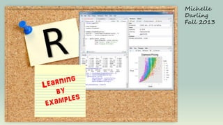
VECTOR
[1]
•
•
•
•
MATRIX
[2]
[3]
1 row, N columns.
One data type only (numeric, character, date, OR logical).
Uses: track changes in a single variable over time.
Examples: stock prices, hurricane path, temp readings, disease spread,
financial performance, sports scores.
[,1]
•
•
•
[,3]
[1,]
[2,]
[3,]
•
•
•
N row, N columns.
One data type only (any combination of numeric, character, date, logical).
Basically, a collection of vectors.
DATA FRAME
LIST
[1]
[,2]
[2]
[,1]
[3]
1 row, N columns. Multiple data types.
Uses: ist detailed information for a person/place/thing/concept.
Examples: Listing for real estate, book, movie, contact, country, stock,
company, etc. Or, a "snapshot" or observation of an event or phenomenon
such as stock market, or scientific experiment.
[,2]
[,3]
[1,]
[2,]
[3,]
•
•
•
N rows, N columns.
Multiple data types.
Basically, a collection of lists or snapshots which when assembled together
provide a "bigger picture."](data:image/gif;base64,R0lGODlhAQABAIAAAAAAAP///yH5BAEAAAAALAAAAAABAAEAAAIBRAA7)
Recomendados
Más contenido relacionado
La actualidad más candente
La actualidad más candente (20)
Destacado
Destacado (20)
Similar a R learning by examples
Similar a R learning by examples (20)
Más de Michelle Darling
Último
Último (20)
R learning by examples
- 2. R data structures VECTOR [1] • • • • MATRIX [2] [3] 1 row, N columns. One data type only (numeric, character, date, OR logical). Uses: track changes in a single variable over time. Examples: stock prices, hurricane path, temp readings, disease spread, financial performance, sports scores. [,1] • • • [,3] [1,] [2,] [3,] • • • N row, N columns. One data type only (any combination of numeric, character, date, logical). Basically, a collection of vectors. DATA FRAME LIST [1] [,2] [2] [,1] [3] 1 row, N columns. Multiple data types. Uses: ist detailed information for a person/place/thing/concept. Examples: Listing for real estate, book, movie, contact, country, stock, company, etc. Or, a "snapshot" or observation of an event or phenomenon such as stock market, or scientific experiment. [,2] [,3] [1,] [2,] [3,] • • • N rows, N columns. Multiple data types. Basically, a collection of lists or snapshots which when assembled together provide a "bigger picture."
- 3. Other important R concepts FACTORS USER-DEFINED FUNCTIONS Stores each distinct value only once, and the data itself is stored as a vector of integers. When a factor is first created, all of its levels are stored along with the factor. > f <- function(a) { a^2 } > f(2) [1] 4 > weekdays=c("Monday","Tuesday","Wednesday","Thursday","Friday") > wf <- factor(weekdays) [1] Monday Tuesday Wednesday Thursday Friday Levels: Friday Monday Thursday Tuesday Wednesday Used to group and summarize data: WeekDaySales <- (DailySalesVector, wf, sum) # Sum daily sales figures by M,T,W,Th,F PACKAGES, FUNCTIONS, DATASETS > search() # Search for installed packages & datasets [1] ".GlobalEnv" "mtcars" "tools:rstudio" [4] "package:stats" "package:graphics" "package:grDevices" • • • • SPECIAL VALUES • • • # List available datasets pi=3.141593. Use lowercase "pi"; "Pi" or "PI" won't work inf=1/0 (Infinity) NA=Not Available. A logical constant of length 1 that means neither TRUE nor FALSE. Causes functions to barf. • Tell function to ignore NAs: function(args, na.rm=TRUE) • Check for NA values: is.na(x) > library(ggplot2) # load package ggplot2 Attaching package: ‘ggplot2’ > data() Functions can be passed as arguments to other functions. Function behavior is defined inside the curly brackets { }. Functions can be nested, so that you can define a function inside another. The return value of a function is the last expression evaluated. • NULL=Empty Value. Not allowed in vectors or matrixes. • > attach(iris) # Attach dataset "iris" • Check for NULL values: is.null(x) NaN=Not a Number. Numeric data type value for undefined (e.g., 0/0). See this for NA vs. NULL explanation.
- 5. VECTORS [1] [2] [3] # 1xN array of same data type > v<-c(1:3); v [1] 1 2 3 > mode(v) # displays data type [1] "numeric" > v <-c("one", "two", "three"); v [1] "one" "two" "three" > mode(v) [1] "character" > v <-c(TRUE,FALSE,TRUE); v [1] TRUE FALSE TRUE > mode(v) [1] "logical" > v<-c(pi, 2*pi, 3*pi); v [1] 3.141593 6.283185 9.424778 > mode(v) [1] "numeric" # Numeric values coerced into character mode > v<-c(1,2,3,"one", "two", "three"); v [1] "1" "2" "3" "one" "two" "three" > mode(v) [1] "character" BASIC OPERATIONS # Addition > v1<-1:3 > v2 <- c(10,10,10) > mode(v1) [1] "numeric" > mode(v2) [1] "numeric" > v1+v2 [1] 11 12 13 # Multiplication & Division > v1 * v2 [1] 10 20 30 > v1 / v2 [1] 0.1 0.2 0.3 > v2 / v1 [1] 10.000000 5.000000 3.333333 #Subtraction > v1-v2 [1] -9 -8 -7 > v2-v1 [1] 9 8 7 # Logical Comparison > v1==v2 [1] FALSE FALSE FALSE > v1 != v2 [1] TRUE TRUE TRUE > v1 > v2 [1] FALSE FALSE FALSE > v1 < v2 [1] TRUE TRUE TRUE
- 6. VECTORS [1] [2] [3] # By default, column numbers are used as indexes > v3[1] [1] 1 # But columns can be given meaningful names… > names(v3) # What are current column names? NULL > names(v3)<- c("1st","2nd","3rd","4th","5th", "6th") # Rename column names. > names(v3) [1] "1st" "2nd" "3rd" "4th" "5th" "6th" > v3 1st 2nd 3rd 4th 5th 6th 1 2 3 10 10 10 # Now we can use names as indexes: > v3["6th"] # same as v3[6] 6th 10 > v3[c("1st","6th")] # same as v3[c(1,6)] 1st 6th 1 10 > v3[-1] # Can exclude columns using (-) 2nd 3rd 4th 5th 6th 2 3 10 10 10 INDEXING, SELECTING & SUBSETTING > v3[v3==10] # Select values equal to 10 [1] 10 10 10 > v3[v3!=10] # Select values NOT equal to 10 [1] 1 2 3 > median(v3) [1] 6.5 > v3[v3<median(v3)] # Select values < median [1] 1 2 3 > v3[v3>median(v3)] # Select values > median [1] 10 10 10 > v3 < median(v3) # Test if value < median? [1] TRUE TRUE TRUE FALSE FALSE FALSE > v3 %% 2==0 # Test if value is an even number? [1] FALSE TRUE FALSE TRUE TRUE TRUE > v3 %% 2==1 # Test if value is an odd number? [1] TRUE FALSE TRUE FALSE FALSE FALSE
- 7. LIST: Examples [1] [2] Product Details Series: O'Reilly Cookbooks Paperback: 438 pages Publisher: O'Reilly Media; 1 edition (March 22, 2011) Language: English ISBN-10: 0596809158 ISBN-13: 978-0596809157 Product Dimensions: 0.9 x 7 x 9.2 inches Shipping Weight: 1.6 pounds [3]
- 8. LISTS [[1]] [[2]] [[3]] # 1xN array of multiple data types/modes > c1 <-c("A", "B", "C") > n1 <-c(1:3) > l2 <- list(c1,n1,Sys.Date(),TRUE);l2 [[1]] [1] "A" "B" "C" [[2]] [1] 1 2 3 [[3]] [1] "2013-11-03" [[4]] [1] TRUE > str(l2) List of 4 $ : chr [1:3] "A" "B" "C" $ : int [1:3] 1 2 3 $ : Date[1:1], format: "2013-11-03" $ : logi TRUE > l2[[4]] [1] TRUE > l2[[1]] [1] "A" "B" "C" ------->fix('l2') list(c("A", "B", "C"), 1:3, structure(16012, class = "Date"),TRUE) # Append to a list; the results get trippy > l2 <- list(l2,pi); l2 [[1]] [[1]][[1]] [1] "A" "B" "C" [[1]][[2]] [1] 1 2 3 [[1]][[3]] [1] "2013-11-03" [[1]][[4]] [1] TRUE [[2]] [1] 3.141593 # Basically, a new () gets added each time the list is appended list(list(c("A", "B", "C"), 1:3, structure(16012, class = "Date"), TRUE), 3.14159265358979) # [[1]] is not the same as [1] > mode(l3[[1]]) [1] "numeric" > mode(l3[1]) [1] "list" # To avoid confusion, use names > l3 = list(x=1,y=2,z=3); l3 $x [1] 1 $y [1] 2 $z [1] 3 > l3$x # this is the same as l3[[1]] [1] 1
- 9. MATRIX: Examples [,1] [1,] [2,] [3,] [,2] [,3] Recommendation Engine Matrices bought bought bought bought likely buy likely buy
- 10. DATA FRAME: Examples [,1] [,2] [,3] [1,] [2,] [3,] Data Frames: Most frequently used structure for storing and manipulating data sets. Similar to: • A database table • A spreadsheet Like the above, DFs have rows x columns, but terminology is different: • Observations = rows • Variables = Columns R Table vs. Data Frame: KISS and stick to data frames for now. #Convert table to data frame: > HEC <- data.frame(HairEyeColor) > str(HEC) 'data.frame':32 obs. of 4 variables: $ Hair: Factor w/ 4 levels "Black","Brown",..: 1 2 3 4 1 2 3 4 1 2 ... $ Eye : Factor w/ 4 levels "Brown","Blue",..: 1 1 1 1 2 2 2 2 3 3 ... $ Sex : Factor w/ 2 levels "Male","Female": 1 1 1 1 1 1 1 1 1 1 ... $ Freq: num 32 53 10 3 11 50 10 30 10 25 ...
- 11. DATA FRAMES [,1] [,2] [,3] [1,] [2,] [3,] # HEC[1,] returns a row > HEC[1,] Hair Eye Sex Freq 1 Black Brown Male 32 # Subsetting made easier > HEC6 <-subset(HEC,select=Hair); str(HEC6) 'data.frame': 32 obs. of 1 variable: $ Hair: Factor w/ 4 levels "Black","Brown",..: 1 2 3 4 > HEC7 <-subset(HEC,select= c(Hair,Eye)); str(HEC7) 'data.frame': 32 obs. of 2 variables: $ Hair: Factor w/ 4 levels "Black","Brown"... $ Eye : Factor w/ 4 levels "Brown","Blue"... > HEC8 <-subset(HEC, subset=(Hair == "Black" & Eye == "Brown")); HEC8 Hair Eye Sex Freq 1 Black Brown Male 32 17 Black Brown Female 36 INDEXING, SELECTING & SUBSETTING # HEC[[1]], HEC[,"Hair"], HEC$Hair return column > HEC1 <-HEC[[1]]; HEC1 > str(HEC1) Factor w/ 4 levels "Black","Brown",..: 1 2 3 4 1 2 3 4 1 2 ... # HEC[1] and HEC["Hair"] return column dframe > HEC2 <-HEC[1]; HEC2 > str(HEC2) 'data.frame':32 obs. of 1 variable: $ Hair: Factor w/ 4 levels "Black","Brown",..: 1 2 3 4 1 2 3 4 1 2 > HEC4 <-HEC["Hair"] > HEC2 == HEC4 Hair [1,] TRUE [2,] TRUE # # > > etc. Returning multiple columns in a data frame This is the same as HEC[,c(1, 4)] HEC5 <-HEC[,c("Hair", "Freq")] str(HEC5) 'data.frame': 32 obs. of 2 variables: $ Hair: Factor w/ 4 levels "Black","Brown",..: 1 2 3 4 1 2 3 4 1 $ Freq: num 32 53 10 3 11 50 10 30 10 25 ...
- 12. DATA FRAMES # Combine 2 DFs columnwise > echo <- cbind(HEC2, HEC4) > echo Hair Hair 1 Black Black 2 Brown Brown 3 Red Red etc # Stack 2 DFs (UNION) > rbind(HEC8, HEC8) 1 17 11 171 Hair Black Black Black Black Eye Sex Freq Brown Male 32 Brown Female 36 Brown Male 32 Brown Female 36 # Skip having to specify the DF for col names > f <- sum(HEC$Freq) # Instead of this > attach(HEC) > f <- sum(Freq) # Use this
- 13. FUNCTIONS SEQUENCING seq(from,to,by) generate a sequence indices <- seq(1,10,2) #indices is c(1, 3, 5, 7, 9) rep(x,ntimes) repeat x n times y <- rep(1:3, 2) # y is c(1, 2, 3, 1, 2, 3) cut(x,n) divide continuous variable in factor with n levels y <- cut(x, 5) DATE PROCESSING Sys.Date() as.date() generate today's date > Sys.Date() [1] "2013-11-03 Convert string to date format > to=as.Date('2006-1-10') > mode(to) [1] "numeric" > class(to) [1] "Date" CHARACTER PROCESSING Description substr(x, start=n1, stop=n2) Extract or replace substrings in a character vector. x <- "abcdef" substr(x, 2, 4) is "bcd" substr(x, 2, 4) <- "22222" is "a222ef" grep(pattern, x , Search for pattern in x. If fixed =FALSE then pattern is ignore.case=FALSE, fixed=FALSE) a regular expression. If fixed=TRUE then pattern is a text string. Returns matching indices. grep("A", c("b","A","c"), fixed=TRUE) returns 2 sub(pattern, replacement,x, Find pattern in x and replace with replacement text. If ignore.case =FALSE, fixed=FALSE) fixed=FALSE then pattern is a regular expression. If fixed = T then pattern is a text string. sub("s",".","Hello There") returns "Hello.There" strsplit(x, split) Split the elements of character vector x at split. strsplit("abc", "") returns 3 element vector "a","b","c" paste(..., sep="") Concatenate strings after using sep string to seperate them. paste("x",1:3,sep="") returns c("x1","x2" "x3") paste("x",1:3,sep="M") returns c("xM1","xM2" "xM3") paste("Today is", date()) toupper(x) Uppercase tolower(x) Lowercase TYPE CONVERSION STRUCTURE CONVERSION as.character(x) as.complex(x) as.numeric(x) as.logical(x) as.data.frame(x) as.list(x) as.matrix(x) as.vector(x)
- 14. DATA TRANSFORMATIONS VECTOR [1] [2] [3] MATRIX # s=simplify into a vector # sapply returns a vector l <- sapply(lst,function) # lapply returns a list v <- lapply(lst,function) [,1] [,3] [1,] [2,] [3,] DATA FRAME LIST [1] [,2] [2] [,1] [3] [1,] [2,] [3,] [,2] [,3]
- 15. GET HELPFUL INFO PRINTING # Get help >help.search("cat") # find info about "cat" >?mean # get help about function >example(mean) # get examples > print(matrix(c(1234),2,2)) [,1] [,2] [1,] 1234 1234 [2,] 1234 1234 # List objects in workspace > ls() [1] "tbl" "w_day" > print(matrix(c(1,2,3,4),2,2)) [,1] [,2] [1,] 1 3 [2,] 2 4 # List all available datasets > data() # Get structure > str(HairEyeColor) table [1:4, 1:4, 1:2] 32 53 10 3 11 50 10 30 10 25 ... - attr(*, "dimnames")=List of 3 ..$ Hair: chr [1:4] "Black" "Brown" "Red" "Blond" ..$ Eye : chr [1:4] "Brown" "Blue" "Hazel" "Green" ..$ Sex : chr [1:2] "Male" "Female" # Get Class (vector,list, dataframe, table, matrix, numeric, function, factor,, et) > class(HairEyeColor) [1] "table" # Use Google R style sheet > print ("print works on only");print("one string or variable at a time"); print(pi) [1] "print works on only" [1] "one string or variable at a time" [1] 3.141593 > num <-1:10 > print(num) [1] 1 2 3 4 5 6 7 8 9 10 # cat works only on strings and vectors > cat("the first 10 numbers are:", num, "n") the first 10 numbers are: 1 2 3 4 5 6 7 8 9 10
- 16. INPUT / OUTPUT Ctrl-R executes the selected line(s) # Getting and setting the working directory > getwd() [1] "C:/Users/mdarling/Documents" > setwd("DA/data") [1] "C:/Users/mdarling/Documents/DA/data" # Enter data using spreadsheet editor w_day <- data.frame() w_day <- edit(w_day) # Read data from URL > tbl <read.csv("http://www.andrewpatton.com/countrylist.csv") # Write data to csv file > write.csv(tbl, "countries.csv") # > > > Read data from HTML tables library(XML) url <-"http://www.andrewpatton.com/countrylist.html" tbls <- readHTMLTable(url) MORE DATE PROCESSING library(timeDate) ymdhs <- "2012-03-04 05:06:07" pd.sec <- as.POSIXlt(ymdhs)$sec pd.hour <- as.POSIXlt(ymdhs)$hour pd.min <- as.POSIXlt(ymdhs)$min pd.mday <- as.POSIXlt(ymdhs)$mday pd.mon <- ((as.POSIXlt(ymdhs)$mon)+1) pd.year <- ((as.POSIXlt(ymdhs)$year) + 1900)
- 17. PLOTTING Plotting in R - base - ggplot2, ggmap, map Types of Graphs - chloropleth - heat map # Base plots plot(faithful, type = 'l') #line graph plot(faithful, type = 'p') #point graph hist(faithful$waiting) #histogram of column waiting # Quickly plot a matrix of scatterplots # This plots each column vs. all the other ones names(iris) [1] "Sepal.Length" "Sepal.Width" "Petal.Length" "Petal.Width" "Species" pairs(iris[,-5]) pairs(iris[,1:2]) # Plot x vs. y using 2 df columnns and geom_point() ggplot(movies, aes(x=year, y=budget)) + geom_point() # Plot histogram using 1 column, Note: geom_bar() ggplot(movies, aes(x=year)) + geom_bar() # plot all rows vs. mpaa column plot(movies[, "mpaa"]) # plot has lots of nulls mpaa.movies <- subset(movies, mpaa != "")! # exclude nulls plot(mpaa.movies[, "mpaa"]) # Or use na.rm