SlideShare a Scribd company logo
1 of 79
Download to read offline
JABATAN KEJURUTERAAN INFRASTRUKTUR DAN GEOMATIK
FAKULTI KEJURUTERAAN AWAM DAN ALAM SEKITAR

3.0

PILE FOUNDATION

3.1

Types of piles and their structural characteristics

1. Steel piles, Figure 3.1
 Consist of pipe piles or rolled steel H-section piles
 The allowable structural capacity of steel piles :
Qall  As f s

Where :

As – cross-sectional area of steel
fs – allowable stress of steel

 Use of additional thickness and epoxy coating are used to
avoid corrosion, and typical condition of splicing (sambat) when
needed is shown in Figure 3.1.

Figure 3.1 Steel Piles
2. Concrete piles
 Two categories of concrete piles are (a) precast and (b) cast-insitu
 Precast piles, Figure 3.2:
-

prepared with ordinary reinforcement
1
JABATAN KEJURUTERAAN INFRASTRUKTUR DAN GEOMATIK
FAKULTI KEJURUTERAAN AWAM DAN ALAM SEKITAR

-

in the shape of square or octagonal

Figure 3.2 Precast piles with ordinary reinforcement
 Cast-in-situ or cast-in-place, Figure 3.3 :
made by driving a steel casing with mandrel into the ground
-

-

upon reaching the desired depth, mandrel is pulled out and the
casing remain
with or without pedestal
uncased piles :
- casing is driven to the desired depth, and filled with
fresh concrete later gradually withdrawn
- with or without pedestal
allowable loads :
cased pile : Qall  As f s  Ac f c
uncased pile : Qall  Ac f c
where :
As – cross sectional area of steel
Ac - cross sectional area of concrete
fs – allowable stress of steel
fc - allowable stress of concrete

Figure 3.3 Cast in place concrete piles
2
JABATAN KEJURUTERAAN INFRASTRUKTUR DAN GEOMATIK
FAKULTI KEJURUTERAAN AWAM DAN ALAM SEKITAR

3. Timber piles
 Three classifications are :
o
o
o

Class A : to carry heavy loads; min butt dia. = 14in
(356mm)
Class B : to carry medium loads; min butt dia. = 12-13in
(305-330mm)
Class C : used as temporary works but permanently for
submerged structure; min butt dia. = 12in (305mm)

 Splicing can be done by means of pipe sleeves or metal straps
or bolts, Figure 3.4
 The allowable load-carrying capacity :
Qall  Ap f w

Where :

Ap – average cross-sectional area of the pile
fw – allowable stress for the timber

Figure 3.4 Splicing of timber piles (a) use of pipe sleeves (b) use of
metal straps and bolts
4. Composite piles
 Upper and lower portions of composite piles are made of
different material
 They may in the form of : steel-cast-in-place concrete or
timber-concrete piles
3
JABATAN KEJURUTERAAN INFRASTRUKTUR DAN GEOMATIK
FAKULTI KEJURUTERAAN AWAM DAN ALAM SEKITAR

5. Pile in term of their function support capacity, Figure 3.5:
(a) Bearing pile, (b) friction pile, (c) piles under uplift,
(d) piles under lateral loads, (e) batter piles under lateral loads



Figure 3.5
 Requirements and conditions for pile foundations, Figure 3.6 :


Figure 3.6 Conditions for use of pile foundations
4
JABATAN KEJURUTERAAN INFRASTRUKTUR DAN GEOMATIK
FAKULTI KEJURUTERAAN AWAM DAN ALAM SEKITAR

- transmit load to the stronger underlying bedrock, 3.6(a)
- gradually transmitting the load to the surrounding soil by
means of frictional resistance at the soil-pile interface, 3.6(b)
- subjected to horizontal load while supporting the vertical load
transmitted by superstructure, 3.6(c)
- built extended into hard stratum under collapsible soil (loess) to
avoid the zone of moisture change that lead to swell and
shrink, 3.6(d)
- to resist uplifting forces for basement mats under water table,
3.6(e)
- to resist scouring at the bridge abutments and piers that can
lead to possible loss of bearing capacity of soil underneath,
3.6(f)
3.2

Estimating Pile Length, Figure 3.7

Figure 3.7 (a) and (b) Point Bearing Piles; and (c) Friction Piles
 Length of pile estimation depending upon the mode of load
transfer to the soil ; namely :
o

Point Bearing Piles

- the ultimate capacity of the piles depends entirely on the
bearing capacity of the hard stratum
- hence the length, L of the pile is fairly well established
5
JABATAN KEJURUTERAAN INFRASTRUKTUR DAN GEOMATIK
FAKULTI KEJURUTERAAN AWAM DAN ALAM SEKITAR

- the ultimate pile load is then; Qu  Q p  Qs (Figure 3.7a)
where :
Qp – load carried at the pile point
Qs – load carried by skin friction developed at the side of the
pile
- piles can be extended into hard stratum with Qu  Q p (Figure
3.7b)
o

Friction Piles

- if no hard stratum presence, piles are driven through softer soil
to specified depths
- resistance to vertical loading, is provided mainly by the skin
friction; (in clayey soil is called adhesion)
- the ultimate load is given by : Qu  Qs
o

Compaction Piles

- piles are driven in granular soil to achieve proper compaction of
soil close to ground surface
- the length depends on :relative density before and after
compaction as well as required depth of compaction

6
JABATAN KEJURUTERAAN INFRASTRUKTUR DAN GEOMATIK
FAKULTI KEJURUTERAAN AWAM DAN ALAM SEKITAR

3.3

Installation of Piles, Figure 3.8

Figure 3.8 Pile driving equipment
 Four method used in piles driving are ; drop hammer, single
acting air or steam hammer, double-acting and differential air
or steam hammer, and diesel hammer
- drop hammer, Figure 3.8a
o raised by a winch, and allowed to drop at a certain height
H
o slow rate of hammer blows
- single acting air or steam hammer, Figure 3.8b
o ram is raised by air or steam pressure and then drops by
gravity
- double-acting and differential air or steam hammer, Figure 3.8c
7
JABATAN KEJURUTERAAN INFRASTRUKTUR DAN GEOMATIK
FAKULTI KEJURUTERAAN AWAM DAN ALAM SEKITAR

o ram is raised and pushed downward by air or steam
pressure
- diesel hammer, Figure 3.8d
o consist of ram, an anvil block and a fuel-injection system
o ram is raised, fuel is injected near the anvil, ram is
released, drops and compresses air-fuel mixture and
ignites it
o this causes; pile to be pushed downward and ram raised
 Vibratory pile driver, Figure 3.8e; consists of counter-rotating
weights that produces centrifugal force that cancel each other
but sinusoidal dynamic vertical force produced pushes the pile
downward
3.4

Pile Load Transfer Mechanism

 Frictional resistance, f(z) with depth is given by :
f z  

Q z 

pz 

Where :
Q z  - increase in pile load

Δz – increase in depth

P – perimeter of pile
 Nature of variation of pile load is as given by Figure 3.9 and
Woo and Juang(1970) has obtained actual variation of load
transfer by a bored concrete pile in Taiwan as in Figure 3.10

8
JABATAN KEJURUTERAAN INFRASTRUKTUR DAN GEOMATIK
FAKULTI KEJURUTERAAN AWAM DAN ALAM SEKITAR

Figure 3.9 Load transfer
mechanism for piles

3.5

Figure 3.10 Load transfer
curves for a concrete
bored pile, Woo and
Juang (1975)

Equations for Estimating Pile Capacity

 Ultimate load-carrying capacity of pile, Qu is :
Qu  Q p  Qs

Where :
Qp – load-carrying capacity of the pile point
Qs – frictional resistance
 Point bearing capacity, Qp is :
*
*
Q p  Ap q p  Ap cN c  q' N q 

Where :
Ap – cross sectional area of pile tip
c – cohesion of the soil supporting the pile tip
qp - unit point cohesion
9
JABATAN KEJURUTERAAN INFRASTRUKTUR DAN GEOMATIK
FAKULTI KEJURUTERAAN AWAM DAN ALAM SEKITAR

q’ =γ’L – effective vertical stress at the level of the pile tip
L- pile length
*
*
N c , N q - the bearing capacity factors
 Frictional resistance, Qs is :
Qs   pLf

Where :
p – perimeter of the pile section
ΔL – incremental pile length where, p and f is constant
f – unit friction resistance at any depth z
 There are many other methods for estimating Qp and Qs
3.6

Meyerhof’s Method – Estimation of Qp

 The value of unit point resistance qp remains constant beyond
the critical embedment ratio, (Lb/D)cr, Figure 3.11

Figure 3.11 Nature of variation of unit point resistance in a
homogeneous sand
 Figure 3.12 is the relationship of (Lb/D)cr and Ø(degree) where
at Ø = 45°, (Lb/D)cr = 25

10
JABATAN KEJURUTERAAN INFRASTRUKTUR DAN GEOMATIK
FAKULTI KEJURUTERAAN AWAM DAN ALAM SEKITAR

 For piles in sand, c=0; but Qp should not exceed Apql,
*
*
Q p  Ap q p  Ap q' N q and Q p  Ap q' N q  Ap ql

 The limiting point resistance is :
SI unit : ql kN / m   50 N tan  ; or English
2

*
q

*
ql lb / ft 2   1000 N q tan 
*
ql kip / ft 2   N q tan 

Where : Ø – soil friction angle in the bearing stratum

Figure 3.12 Nature of variation of unit
point resistance in sand

Figure 3.13 Variation of the
maximum values of

*
N q with Ø

 Using SPT method (Meyerhof, 1976):
q p kN / m 2   40N L / D  400 N

where N - average SPT number at 10D above and 4D below
the pile point.
 For piles in clay, with saturated and undrained conditions
(Ø=0)
*
Q p  N c cu Ap  9cu Ap

Where : cu – undrained cohesion (undrained shear strength) of
the soil below the pile tip

11
JABATAN KEJURUTERAAN INFRASTRUKTUR DAN GEOMATIK
FAKULTI KEJURUTERAAN AWAM DAN ALAM SEKITAR

3.7

Vesic’s Method – Estimation of Qp

 Vesic (1977) proposed value of Qp as :
*
'
*
Q p  Ap q p  Ap cN c   o N 

Where :
 1  2K o 
'
 o - mean normal ground effective stress = 
q '
 3 

Ko – earth pressure coefficient = 1 – sin Ø
*
N , N  - bearing capacity factors (see Table D.6 of Das textbook)
*
c

3.8

Janbu’s Method – Estimation of Qp

NOT to be covered

 Janbu (1976) proposed value of Qp as :
*
*
Q p  Ap cN c  q' N q 

Where :
*
*
N c , N q - bearing capacity factors, Figure 9.14

Figure 3.14 (a)Meyerhof’s and (b) Janbu’s bearing capacity factors

12
JABATAN KEJURUTERAAN INFRASTRUKTUR DAN GEOMATIK
FAKULTI KEJURUTERAAN AWAM DAN ALAM SEKITAR

3.9

Coyle and Castello’s Method (Estimation of Qp in Sand) NOT TO
BE COVERED

 Coyle and Castello (1981) proposed value of Qp as :
*
Q p  q' N q Ap

Where :
q’ – effective vertical stress at the pile tip
*
N q - bearing capacity factor, Figure 3.15

13
JABATAN KEJURUTERAAN INFRASTRUKTUR DAN GEOMATIK
FAKULTI KEJURUTERAAN AWAM DAN ALAM SEKITAR
*
Figure 3.15 Variation of N q with L/D, unit frictional resistance and K
value for piles in sand (Coyle and Castello, 1981)

3.10 Frictional Resistance, Qs in Sand
 Frictional resistance is, Qs   pLf
 Factors to be kept in mind while estimating unit frictional, f
-

the nature of pile installation
unit skin friction increases with depth
at similar depth, bored or jetted piles has a lower unit
skin friction compared to driven piles

 Approximation of f : (Figure 3.15)
For z = 0 to L’ :
For z = L’ to L :

f  K v' tan 

f  f z L'

Where :
K – effective earth coefficient
 v' - effective vertical stress at specified depth
 - soil-pile friction angle
L’ = 15d
 Read text for values of K, fav and Qs between 1976 and 1982
3.11 Frictional Resistance, Qs in Clay
 Three method of estimating Qs in Clay :
1.  Method :
- proposed by Vijayvergia and Focht (1972)
- assumption : displacement of soil caused by pile driving results
in a passive lateral pressure at any depth
- average unit skin resistance as :

14
JABATAN KEJURUTERAAN INFRASTRUKTUR DAN GEOMATIK
FAKULTI KEJURUTERAAN AWAM DAN ALAM SEKITAR



'

f av    v  2cu



Where :
 v' - mean effective vertical stress for entire embedment length,


A1  A2  A3  ......
L

cu – mean undrained shear strength (Ø=0)
 - refer to Figure 3.16b
- total frictional resistance is : Qs  pLf av

Figure 3.16a Critical embedment ratio and bearing capacity factors
for various soil friction angles, (Meyerhof, 1976).

15
JABATAN KEJURUTERAAN INFRASTRUKTUR DAN GEOMATIK
FAKULTI KEJURUTERAAN AWAM DAN ALAM SEKITAR

Figure 3.16b Variation of  with pile embedment length and its
application, (McCleland – 1974).
2.  Method :
- unit skin resistance in clayey soil is : f  cu
 - empirical adhesion factor, Figure 3.17

α

16
JABATAN KEJURUTERAAN INFRASTRUKTUR DAN GEOMATIK
FAKULTI KEJURUTERAAN AWAM DAN ALAM SEKITAR

Figure 3.17 Variation of  with undrained cohesion of clay
- total frictional resistance is : Qs   fpL  cu pL
3.  Method :
- assumption : excess pore water pressure in normally
consolidated clay for driven pile shall dissipates gradually
- thus unit frictional resistance for the pile is :
f   v'

Where :
 v' - vertical effective stress = γ’z
  K tan  R

ØR – drained friction angle of remolded clay
K – earth pressure coefficient
Where : K  1 sin  R for normally consolidated clays
K  1 sin  R  OCR for overly consolidated clays
- total frictional resistance is : Qs   fpL
3.12 Point Bearing Capacity of Piles Resting on Rock
 Goodman (1980) has approximate the ultimate unit point
resistance in rock as :
q p  qu N  1

Where :
N  tan 2 45   / 2

qu – unconfined compression strength of rock
 - drained angle of friction

17
JABATAN KEJURUTERAAN INFRASTRUKTUR DAN GEOMATIK
FAKULTI KEJURUTERAAN AWAM DAN ALAM SEKITAR

 After taking care of scale effect, qu ( design) 

qu (lab)
5

 Table 3.1 is the typical value of qu(lab) for rocks and Table 3.2
the value of angle of friction respectively
Table 3.1 Typical unconfined compressive strength of rocks
qu
lb/in2

MN/m2

10,000 – 20,000
15,000 – 30,000
5,000 – 10,000
20,000 – 30,000
8,500 – 10,000

Rock type
Sandstone
Limestone
Shale
Granite
Marble

70 – 140
105 – 210
35 – 70
140 – 210
60 – 70

Table 3.2 Typical Values of angle of friction, Ø, of rocks
Rock type
Sandtone
Limestone
Shale
Granite
Marble

Angle of friction, Ø
27 – 45
30 – 40
10 – 20
40 – 50
25 - 30

 Hence, with FS = 3, the allowable point bearing capacity, Qp is :
Q p ( all) 

q

u ( design)

N





 1 Ap

FS

Table 3.3 Typical pre-stressed concrete pile in use

18
JABATAN KEJURUTERAAN INFRASTRUKTUR DAN GEOMATIK
FAKULTI KEJURUTERAAN AWAM DAN ALAM SEKITAR

Table 3.4 : Bearing capacity factors for deep foundations, N*c and N*σ,
Vesic’s, 1977.

19
JABATAN KEJURUTERAAN INFRASTRUKTUR DAN GEOMATIK
FAKULTI KEJURUTERAAN AWAM DAN ALAM SEKITAR

Table 3.5 Janbu’s bearing capacity factors

20
JABATAN KEJURUTERAAN INFRASTRUKTUR DAN GEOMATIK
FAKULTI KEJURUTERAAN AWAM DAN ALAM SEKITAR

Example 3.1
Given : A square 305 mm x 305 mm concrete pile and 12 m long.
Fully embedded in homogeneus sand layer, γd = 16.8 kN/m3 ,
c=0 and Øavg=35°. The average SPT value near pile tip is 16.
Find : a. Qp using Meyerhof’s, Vesic’s, Janbu’s and SPT method.
b. Qs using Qs   pLf and

f  K v' tan  ..( for ..z  0  L' )
f  f z  L ' ...( for ...z  L'  L)

if K=1.3

and   0.8 .
c. Estimate the load-carrying capacity of pile, Qall if FS=4.
d. Qall using Coyle and Costello’s method
Solution :
a. Meyerhof’s :
Because it is a homogeneous soil, Lb=L. For Ø=35°,
(Lb/D)cr =(L/D)cr ≈ 10 (Figure 3-16a). So for this pile, Lb/D = 39.34 >
*
(Lb/D)cr. Hence, from the same figure N q  120
*
Q p  Ap q p  Ap q' N q  0.0929201.6120  2247.4kN

*
ql kN / m 2   50 N q tan   50120tan 35  4201.25kN / m 2

*
Q p  Ap ql  0.09294201  390.3kN  Ap q' N q

Qp = 390 kN
*
Vesic’s : use I rr  90 ; with Ø=35°; N  79.5 so :

1  21  sin  
'
*
*
Q p  A p o N   A p 
 q' N 
3


1  21  sin 35
 0.0929
 201.679.5  923kN
3


*
Janbu’s : with c=0; use  '  90;..and ..  35;..N q  41.3 by int erpolation 
*
Q p  Ap q' N q  0.0929m 2 201.6kN / m 2 41.3  773.5kN

SPT method :

q p kN / m 2   40N L / D  400 N

Q p  Ap q p  0.0929m 2 401639.34  2339kN

21
JABATAN KEJURUTERAAN INFRASTRUKTUR DAN GEOMATIK
FAKULTI KEJURUTERAAN AWAM DAN ALAM SEKITAR

Limiting value = Q p  Ap 400 N  0.0929m 2 40016  595kN
For design purpose : Q p 

595kN  773.5kN  390kN
 586kN
3

b. from sub-topic 3.10 from the note :
L'  15D  150.305m  4.58m

For z = 0 :  v'  0; f  K v' tan   0
For z = L’ to L :

 v'  L'  16.8kN / m 3 4.58m  76.94kN / m 2

f  K v' tan   1.376.94tan0.8  35  53.2kN / m 2

Thus
 f  f z  4.58m 
Qs   z  0
 pL' f z  20 ft pL  L'
2


2
 0  53.2kN / m 
4  0.305m 4.58m   53.2kN / m 2 4  0.305m 12  4.58m 
: 


2







 149  482  631kN

c. thus load carrying capacity of pile, Qu = Qp(avg) + Qs
Q p ( avg )  586kN and Qs  631kN;.....Qall 

Qult 586  631

 304.25kN
FS
4

d. Coyle and Castello’s
*
Qult  Q p  Qs  q' N q Ap  K v' tan0.8  pL;....and ...

L
12

 39.3
D 0.305

*
For Ø=35° and L/D=39.3; N q  40 K≈1.0
Thus :

*
Qult  Q p  Qs  q' N q A p  K v' tan0.8  pL



 



 201.6kN / m 2 40  0.0929m 2
 1.016.8  12  tan0.8  354  0.30512 
 749  1569  2318kN

And Qall 

Qult 2318

 579.6kN
FS
4

22
JABATAN KEJURUTERAAN INFRASTRUKTUR DAN GEOMATIK
FAKULTI KEJURUTERAAN AWAM DAN ALAM SEKITAR

Example 3.2
Given : A driven pile in clay
as in Figure E9.2. The pipe
pile has outside diameter of
406mm and wall thickness
of 6.35mm.

Find :

a. Net point bearing capacity.
b. Skin resistance using α, λ and β method if ØR =30°; the
top 10m is normally consolidated clay and the bottom
clay layer has OCR=2.
c. Net allowable pile capacity, Qall if FS=4.

Solution :
a. Cross section of pile, Ap 



D2 



0.4062  0.1295m 2

4
4
*
Q p  Ap q p  Ap N c cu ( 2)  0.12959100  116.55kN

b. Skin resistance, Qs :
(α method) :

Qs   fpL  cu pL

From Figure α vs cu : cu(1)=30kN/m2 α=1.0; cu(2)=100 α=0.5
Thus :
Qs   fpL   cu pL   1cu (1)  0.40610   2 cu ( 2)  0.40620
 130 0.40610  0.5100 0.40620  1658.2kN

(λ method) : where f av    v'  2cu ( av) 
cu ( avg ) 

cu (1) 10  cu ( 2) 20
30



3010  10020
 76.7kN / m 2
30

Use the plotted Figure E9.2b, for σ’v vs depth;
'

v 

A1  A2  A3 225  552.38  4577

 178.48kN / m 2
L
30

23
JABATAN KEJURUTERAAN INFRASTRUKTUR DAN GEOMATIK
FAKULTI KEJURUTERAAN AWAM DAN ALAM SEKITAR

From Figure λ vs L; λ=0.14 for L=30m; so

f av    v'  2cu ( av)   0.14178.48  276.7  46.46kN / m 2

Hence; Qs  pLf av   0.4063046.46  1777.8kN
(β method) : where ØR =30°; f   v' ;   K tan  R ; K  1 sin  R
K  1 sin  R  OCR

For z=0-5m :
 0  90 
2
f av(1)  1  sin  R  tan  R v' ( av)  1  sin 30tan 30
  13.0kN / m
2 


For z=5-10m :
 90  130.95 
2
f av( 2)  1  sin  R  tan  R v' ( av)  1  sin 30tan 30
  31.9kN / m
2



For z=10m-30m , OCR=2:
 130.95  326.75 
2
f av(3)  1  sin  R  tan  R OCR v' ( av)  (1  sin 30)tan 30 2 
  93.43kN / m
2



so





Qs  p f av(1) 5  f av( 2) 5  f av(3) 20   0.406135  31.95  93.4320  2669.7kN

c. So use α and λ method which produced almost similar results,
Qs 

1658.1  1777.8
 1718kN
2

Qult  Q p  Qs  116.46  1718  1834.46kN;....hence...Qall 

Qult 1834.46

 458.6kN
FS
4

Example 3.3
Given : An H-pile (size HP 310 x 1.226), length of embedment =
26m, driven through soft clay and rest on sandstone, qu(lab) for
sandstone = 76 MN/m2, Ø=28°, FS=5.
Find : The allowable point bearing capacity, Qp(all)
Solution : Since q p  qu N  1 ; N  tan 2 45   / 2 and qu ( design) 

qu (lab)
5



  
 qu ( lab)  
2

 tan  45    1  A p
5 
2
q p Ap
qu N   1A p





Q p ( all ) 

 
FS
FS
FS
 76  10 3 kN / m 2  

28 
2
3
2
  1  15.9  10 m

  tan  45 
5
2 





 
 182kN
5





24
JABATAN KEJURUTERAAN INFRASTRUKTUR DAN GEOMATIK
FAKULTI KEJURUTERAAN AWAM DAN ALAM SEKITAR

EXAMPLE OF FINAL EXAMINATION QUESTION
Q4 The most common function of piles is to transfer a load that cannot be adequately
supported at shallow depths to a depth where adequate support becomes available.
Hence, the piles can also be categorized based on its function/ support capacity.
(a)

Briefly describe with relevant sketches the five (5) functions / support
capacity of piles.
(5 marks)

(b)

Reinforced concrete piles 18 m long, of square section and width 400 mm
are driven through 8 m of loose fill with unit weight of 13 kN/m3 to
penetrate 10 m into an underlying firm to stiff saturated clay. The
groundwater table is found at a depth of 2 m below ground surface.

(i)

Determine the ultimate bearing capacity, Qult, of pile by the given formula,
if the undrained shear strength of the clay increases linearly with depth
from 65 kN/m2 at the top of the clay to 100 kN/m2 at a depth of 10 m
below the surface of the clay.
Assuming that the unit weight of stiff saturated clay is 17 kN/m3
throughout the layer and the frictional capacity of the loose fill is
negligible.
(10 marks)

(ii)

Assuming that it is necessary to provide a number of such piles to carry
the total foundation load, explain the bearing capacity of the pile group is
estimated? Discuss your answer with the help of relevant sketches.
(5 marks)

25
JABATAN KEJURUTERAAN INFRASTRUKTUR DAN GEOMATIK
FAKULTI KEJURUTERAAN AWAM DAN ALAM SEKITAR
ANSWER
Q4

The most common function of piles is to transfer a load that cannot be adequately
supported at shallow depths to a depth where adequate support becomes available.
Hence, the piles can also be categorized based on its function/ support capacity.
(a)

Briefly describe with a relevant sketch what are the five (5) function/
support capacity of piles.
(5 marks)

(a) Bearing pile, (b) friction pile, (c) piles under uplift,
(d) piles under lateral loads, (e) batter piles under lateral loads
(b)

A reinforced concrete piles 18 m long, of square section and width 400
mm is driven through 8 m of loose fill with unit weight of 13 kN/m3 to
penetrate 10 m into the underlying firm to stiff saturated clay. The
groundwater table is found at a depth of 2 m below ground surface.
(i)

Determine the ultimate bearing capacity, Qult of pile by the given
formula, if the undrained shear strength of the clay increases

26
JABATAN KEJURUTERAAN INFRASTRUKTUR DAN GEOMATIK
FAKULTI KEJURUTERAAN AWAM DAN ALAM SEKITAR
linearly with depth from 65 kN/m2 at the top of the clay to 100
kN/m2 at a depth of 10 m below the surface of the clay.
Assuming that the unit weight of firm to stiff saturated clay is 17
kN/m3 throughout the layer and the frictional capacity of the loose
fill is negligible.
Given that:-





qtip = cu Nc (Based on Meyerhof’s equation); f s ( avg )    v '  2cu
(10 marks)
Answer:To determine Qp:qtip = cu Nc = 100 kN/m2 x 9 = 900 kN/m2

[1M]

Ap = 0.4 x 0.4 = 0.16 m2

[1M]

Qp = Apqtip = 0.16 x 900 = 144 kN

[0.5M]

To determine Qs:-

(45.14  117.04)(10)
2
v' 
 81.09kN / m 2
10
Elevation (m)
0
2
8
18

[1M]

Effective Vertical Pressure (kN/m2)
0
26
45.14
117.04
[1M]

(65  100)(10)
2
cu 
 82.5kN / m 2
10
Based on Figure 1,  = 0.185



[1M]
[1M]



f s ( avg )    v '  2cu
= (0.185)[81.09+2(82.5)]
= 45.53kN/m2
As = 4 x 0.4 x 10 = 16 m2

[1M]
[0.5 M]

27
JABATAN KEJURUTERAAN INFRASTRUKTUR DAN GEOMATIK
FAKULTI KEJURUTERAAN AWAM DAN ALAM SEKITAR
Qs = As. fs = 16 x 45.53 = 728.48 kN

[1M]

Qult = Qs + Qp = 728.48 + 144
= 872.48 kN

[1M]

(ii)

Assuming that it is necessary to provide a number of such piles to
carry the total foundation load, how could the bearing capacity of
the pile group be estimated? Discuss your answer with a relevant
sketch.
(5 marks)

Answer:For most practical purposes, the ultimate load of pile group, (QvG)ult, can be estimated
based on the smaller value of the following two values:(a) Group Action – block failure (Figure A) of pile group by
breaking into the ground along an imaginary perimeter and bearing
at the base. The ultimate capacity for the group failure can be
estimated from the following relationship:(QvG)ult =  x n x (Qv)ult
[2M]
(b) Individual Action (Figure B) – if there is no group action
(when the center to center spacing, s, is large enough, >1), in that
case, the piles will behave as individual piles. The total load of the
group can be taken as n times the load of the single pile, in which
(QvG)ult = n x (Qv)ult =  (Qv)ult
[2M]

28
JABATAN KEJURUTERAAN INFRASTRUKTUR DAN GEOMATIK
FAKULTI KEJURUTERAAN AWAM DAN ALAM SEKITAR

Figure : (A) Individual action, (B) Group action
[2 x 0.5M = 1M

3.13 Pile Load Test
 Pile load test arrangement by means of hydraulic jack is shown
in Figure 3.18a
 Step loads are applied to the pile, so that a small amount of
settlement is allowed to occur
 Settlement from field test is recorded as in Figure 3.18b
 Net settlement calculation for any load Q :
- When Q = Q1 : Net settlement, snet(1)  st (1)  se(1)
29
JABATAN KEJURUTERAAN INFRASTRUKTUR DAN GEOMATIK
FAKULTI KEJURUTERAAN AWAM DAN ALAM SEKITAR

- When Q = Q2 : Net settlement, snet( 2)  st ( 2)  se( 2)
Where :
snet – net settlement
se – elastic settlement of the pile itself
st – total settlement
 The values of Q then plotted against se produces diagram in
Figure 3.18c

Figure 3.18 (a) Test arrangement (b) load vs total settlement
(c) load vs net settlement
3.14 Failure criteria of a pile
 The ultimate failure load for a pile is defined as the load when
the pile plunges or the settlements occur rapidly under
sustained load and the amount of settlement exceed the
acceptable soil-pile system
 Or
 Besides it, many engineers define the failure load at the point
of intersection of the initial tangent to the load-settlement
curve and the tangent to or the extension of the final portion of
the curve.

30
JABATAN KEJURUTERAAN INFRASTRUKTUR DAN GEOMATIK
FAKULTI KEJURUTERAAN AWAM DAN ALAM SEKITAR

 Arbitrary settlement limits that the pile is considered to have
failed when the pile head has moved 10 percent of the pile end
diameter or the gross settlement of 1.5 in. (38 mm) and net
settlement of 0.75 in. (19 mm) occurs under two times the
design load. (JKR standard)

 However, all of these definitions for defining failure are
judgemental.
3.15 Pile Driving Formulas
 Due to varying soil profiles layers a point bearing pile cannot
always satisfied the capability of penetrating the dense soil to a
predetermined depth; therefore several equations have been
developed by many to calculate the ultimate capacity of pile
during driving.
 According to Engineering News Record (ENR), Qu is :
Qu 

WR h
S C

Where :
WR – weight of the ram
h – height of fall of the ram
S – penetration of pile per hammer blow (from last few
driving blows)
C – a constant
(for drop hammers : C = 1 in. ; S and h are in inches)
(for steam hammers : C = 0.1 in. ; S and h are in inches)
FS = 6
For single and double-acting hammers WRh is replaced by EHE
Thus :
Qu 

EH E
S C

Example 3.4
A precast concrete pile 12 in. x 12 in. in cross section is driven by a
hammer. Given :
Maximum rated hammer energy = 30 kip-ft
Hammer efficiency = 0.8
31
JABATAN KEJURUTERAAN INFRASTRUKTUR DAN GEOMATIK
FAKULTI KEJURUTERAAN AWAM DAN ALAM SEKITAR

Weight of ram = 7.5 kip
Pile length = 80 ft
Coefficient of restitution = 0.4
Weight of pile cap = 550 lb
Ep = 3 x 10⁶ kip/in2
Number of blows for last 1 in. of penetration = 8
Estimate the allowable pile capacity by the
a. Modified ENR formula (use FS=6)
b. Danish formula (use FS = 4)
c. Gates formula (use FS = 3)
Solution :
a.
Weight of pile + cap = 12  12  80150lb / ft 3   550  12.55kip
12
12
and WR h  30kip  ft
2
EW R h WR  n W p 0.830  12kip  in  7.5  0.42 12.55
Qu 

 607kip
1
S  C WR  W p
7.5  12.55
8  0.1

Qall 

b.

Qu 607

 101kip
FS
6
EH E
Qu 
EH E L
S
2 Ap E p

Use Ep = 3 x 10⁶ lb/in2
And

Qu 
Qall

c.

EH E L

2 Ap E p

0.830  1280  12
 3  10 6

212  12
kip / in 2 
 1000




 0.566in.

0.830  12  417kip

 0.566
417

 104kip
4
1
8

Qu  a EH E b  log S   27 0.8301  log1   252kip
8
252
Qall 
 84kip
3

3.16 Hiley’s Formula for estimating single RC pile capacity.
32
JABATAN KEJURUTERAAN INFRASTRUKTUR DAN GEOMATIK
FAKULTI KEJURUTERAAN AWAM DAN ALAM SEKITAR

The Hiley’s formula gives the simplest method of calculating the final
setting or the ultimate load of a pile while driving depending upon
the given parameter.
It is usually written as :
BW H h WH  Pe 2
C
s 

2 FS  WL
WH  P

And
C  Cc  C p  C q

where :
s
C
WH
h
P
P1
P2
WL
FS
e
Cc

- Set value /1 blow (mm/blow)
- Temporary compression of pile & soil (mm)
- Weight of hammer (kN)
- Drop of hammer (mm)
- Total load (P1 + P2) (kN)
- Weight of pile (kN)
- Weight of driving assembly (kN)
- Pile working load (kN)
- Factor of safety
- Coefficient of restitution
- Temporary compression coefficient due to pile
head and cap (mm), Table 3.3
Cp, - Temporary compression coefficient due to pile
length (mm), Table 3.3
Cq, - Temporary compression coefficient due to ground
or quake (mm), Table 3.3

Note :
(a)

(b)
(c)
(d)

This formula was developed by Hiley (1925). The formula
assumes the energy of the falling hammer during pile
driving is proportional resisted by the pile. This method is
widely considered to be one of the better formulas that
intended to be applied to cohesionless, well-drained soils
or rock.
Weight of the hammer shall be about 0.5 to 2.0 times of
the total pile weight.
The term mass and weight are interchangeably
The term Cp and Cq are shown in Figure 3.19 after a pile
set measurement of pile are made.

33
JABATAN KEJURUTERAAN INFRASTRUKTUR DAN GEOMATIK
FAKULTI KEJURUTERAAN AWAM DAN ALAM SEKITAR

Figure 3.19 : Example graph of pile set
Table 3.6 : Values of Cc, Cp and Cq
Form of
compression

Pile head
and cap, Cc

Pile length,
Cp

Quake, Cq

Material

Head of timber
pile
Short dolly in
helmet or
driving cap
3 in/76.2mm
packing under
helmet or
driving cap
1 in/25.4mm
pad only on
head of
reinforced
concrete pile
Timber pile
(E=1,500,000
lb/in2) or
(E=10,342,500
kPa)
Pre-cast pile
(E=2,000,000
lb/in2) or
(E=13,790,000
kPa)
Steel pile for
cast in place
(E=30,000,000
lb/in2) or
(E=206,850,000
kPa)
Ground
surrounding pile
and under pile

Easy
driving
(inch)

Medium
driving
(inch)

Hard
driving
(inch)

Very hard
driving
(inch)

0.05

0.10

0.15

0.20

0.05

0.10

0.15

0.20

0.07

0.15

0.22

0.30

0.03

0.05

0.07

0.10

0.004L

0.008L

0.012L

0.016L

0.003L

0.006L

0.009L

0.012

0.003L

0.006L

0.009L

0.012

0.05

0.10 –
0.20

0.15 –
0.25

0.05 –
0.15

34
JABATAN KEJURUTERAAN INFRASTRUKTUR DAN GEOMATIK
FAKULTI KEJURUTERAAN AWAM DAN ALAM SEKITAR
point
Note :
Length, L measure in feet
1 feet = 0.3048 m
1 inch = 25.4 mm
Table 3.7 : Coefficient of restitution, e.
Description

Coefficient of restitution, e

Piles driven with double acting hammer
-

Steel piles without driving cap
Reinforced concrete pile without helmet but with
packing on top of pile
Reinforced concrete piles with short dolly in helmet
and packing
Timber pile

0.5
0.5
0.4
0.4

Piles driven with single acting and drop hammer
-

Reinforced concrete piles without helmet but with
packing on top of piles
Steel piles or steel tube of cast in place piles fitted
with driving cap and short dolly covered by steel plate
Reinforced concrete piles with helmet and packing,
dolly in good condition
Timber pile in good condition
Timber pile in poor condition

0.4
0.32

0.25
0.25
0.00

Example 3.5
Using Hiley’s formula calculate the final set of a 200mm X 200mm RC pile.
The pile driven with single acting and drop hammer with medium driving. The
type of pile is the reinforced concrete pile with helmet and packing, dolly in
good condition.
Other data and parameters are :
Pile working load,
Mass of hammer,
Factor of safety, FS
Pile length, L
Mass driving assembly,
Drop of hammer,
Hammer efficiency,

= 275 kN
= 25 kN
= 2.0
= 18 m
= 2.0 kN
= 400 mm
= 85%
35
JABATAN KEJURUTERAAN INFRASTRUKTUR DAN GEOMATIK
FAKULTI KEJURUTERAAN AWAM DAN ALAM SEKITAR
Density of concrete,

= 24 kN/m3

Solution :
Mass of pile, P1

= Concrete density X Area X Length of pile
= 24 X (0.2 X 0.2) X 18
= 17.28 kN

Total load, P

= P1 + P2
= 17.28 + 2.0
= 19.28 kN

Value of e

= 0.25 (Table 3.7)

BW H h
0.8525400  15.454mm

FS  WL
2.0  275
WH  Pe 2 25  19.28  0.252

 0.592
WH  P
25  19.28

Value of C
Cc
Cp
Cq

:
= 0.15in X 25.4 = 3.81 mm
= 0.006(59ft) = 0.354in X 25.4 = 8.99 mm
= 0.10in X 25.4 = 2.54 mm

C = Cc + Cp + Cq = 3.81 + 8.99 + 2.54 = 15.34 mm
BW H h WH  Pe 2
C
s 

2 FS  WL
WH  P
15.34
 15.454  0.592
2
 s  1.48mm / blow
 or S  14.8mm / 10blow ( Final Set )

Using  s 

Example 3.6
Given :

36
JABATAN KEJURUTERAAN INFRASTRUKTUR DAN GEOMATIK
FAKULTI KEJURUTERAAN AWAM DAN ALAM SEKITAR

A 200mm x 200mm RC square pile. The pile driven with single-acting
and drop hammer with hard driving. The type of pile is reinforced
concrete pile with helmet and packing, dolly in good condition.
Mass of hammer, Wn
Factor of safety, FS
Pile length, l
Mass Driving assembly,P2
Drop hammer, h
Hammer efficiency, B
Set value, S

=25kN
=2.0
=24m
=3.0 kN
=500mm
=85%
=19mm/10 blow (Figure 3.20)

Figure 3.20
Required : Ultimate load of pile
Solution :
Mass of pile, P1 = Concrete densityxAreaxlength
= 24x(0.2x0.2)x24=23.04kN
Total load, P2
Value of e
Cp + Cq
Cc
Temporary
compression, C
Set value, s

=
=
=
=

P1 + P2 = 23.04 + 3=26.04kN
0.25 (Table 3.7)
20mm (Figure 3.20)
0.22inx25.4=5.59mm

= 5.59 + 20 = 25.59mm
= 19mm/10 blow =1.9mm/blow

37
JABATAN KEJURUTERAAN INFRASTRUKTUR DAN GEOMATIK
FAKULTI KEJURUTERAAN AWAM DAN ALAM SEKITAR

BW H h



0.8525500

1
 1



FS  s  C c  C p  C q  2.01.9  25.59
2
 2



2
2
WH  Pe
25  26.040.25

 0.5217
WH  P
25  26.04

 361.52kN

By using Hiley’s equation :
WL 

WH  Pe 2
 361.52  0.5217  188.6kN
 1
 WH  P
FS  s  C p  C q  C c 
 2

BW H h



Therefore, the pile working load must be less than 188.6kN
3.17 Settlement of Piles, Vesics (1969)
 Settlement of a pile under vertical working load, Qw is :
s  s1  s 2  s3

Where :
s – total pile settlement
s1 – elastic settlement of pile
s2 – settlement caused by the load at the pile tip
s3 – settlement caused by the load transmitted along pile shaft
 Formulae :
- elastic settlement, s1 :
s1 

Q

wp

 Qws L
Ap E p

Where :
Qwp – load carried at the pile point under working condition
Qws – load carried by frictional resistance under work load
Ap – area of pile cross section
L – length of pile
Ep – modulus of elasticity of the pile material
 - nature of unit skin friction (=0.5 or 0.67), Figure 3.21

38
JABATAN KEJURUTERAAN INFRASTRUKTUR DAN GEOMATIK
FAKULTI KEJURUTERAAN AWAM DAN ALAM SEKITAR

Figure 3.21 Various types of unit friction resistance along pile shaft
- load at pile point, s2 :
s2 

q wp D
Es

1   I
2
s

wp

Where :
D – width or diameter of pile
qwp – point load per unit area = Qwp/Ap
Es – modulus of elasticity of soil at or below the pile point
μs – Poisson’s ratio of soil
Iwp – influence factor = 0.85
Or
s2 

Qwp C p
Dq p

Where :
qp – ultimate point resistance of the pile
Cp – an empirical coefficient, Table 3.8
Table 3.8 Typical Values of Cp
Soil type
Sand (dense to loose)
Clay (stiff to soft)
Silt (dense to loose)

Driven Pile
0.02-0.04
0.02-0.03
0.03-0.05

Bored Pile
0.09-0.18
0.03-0.06
0.09-0.12

- load carried by pile shaft, s3 :
Q  D
2
s3   ws 
 pL  E 1   s I ws

 s





Where :
39
JABATAN KEJURUTERAAN INFRASTRUKTUR DAN GEOMATIK
FAKULTI KEJURUTERAAN AWAM DAN ALAM SEKITAR

p – perimeter of the pile
L – embedded length of pile
Iws – influence factor = 2  0.35
Or
s3 

L
D

and Cs (a constant) = 0.93  0.16 L / D C p

Qws C s
Lq p

Cp from Table 3.8
Example 3.7
Given : A pre-stressed concrete pile 21m long, being driven into
sand. Working load, Qw = 502 kN. The pile is octagonal in shape with
D = 356 mm, see Figure E9.4. Skin resistance, Qs carries 350 kN, and
Qp carries the rest. Use Ep = 21 x 106 kN/m2, Es = 25 x 103 kN/m2, μs
= 0.35 and ξ = 0.62.
Find : The settlement of the pile.
Solution :
From Table D3; for D=356mm, Ap=1045cm2, p=1.168mm and
Qws=350 kN; so Qwp=502-350=152 kN
Due to material :
s1 

Q

 Qws L

wp

Ap E p



152  0.6235021  0.00353m  3.35mm



0.1045m 2 21  10 6



q wp 

Qwp
Ap

Due to point load :
s2 

q wp D
Es

1   I
2
s

wp





 152  0.356 

1  0.35 2 0.85  0.0155m  15.5mm

3 
 0.1045  25  10 

Due to skin :
With I ws  2  0.35

L
21
 2  0.35
 4.69
D
0.356

40
JABATAN KEJURUTERAAN INFRASTRUKTUR DAN GEOMATIK
FAKULTI KEJURUTERAAN AWAM DAN ALAM SEKITAR
Q  D
 350  0.356 
2
2
s3   ws 
 pL  E 1   s I ws  1.16821 25  10 3  1  0.35 4.69
And




 s
 0.00084mm  0.84mm









Therefore the total settlement is :

s  s1  s2  s3  3.35  15.5  0.84  19.69mm
3.18 Pullout Resistance of Piles
 The gross ultimate resistance of a pile subjected to uplifting
force, Figure 3.22 is :
Tug  Tun  W

Where :
Tug – gross uplift capacity
Tun – net uplift capacity
W – effective weight of pile

Figure 3.22 Uplift capacity of piles
a.

In Clay


Das and Seeley (1982), estimated Tun as :
41
JABATAN KEJURUTERAAN INFRASTRUKTUR DAN GEOMATIK
FAKULTI KEJURUTERAAN AWAM DAN ALAM SEKITAR

Tun  Lp ' cu

Where :
L – length of the pile
p – perimeter of pile section
 ’- adhesion coefficient at soil-pile interface
cu – undrained cohesion of clay
Values of  ' :


-

for cast-in-situ: (for bore pile)
2
 '  0.9  0.00625cu for cu ≤ 80 kN/m
2
 ' 0.4 for cu > 80kN/m

-

for pipe piles :

 '  0.715  0.0191cu for cu ≤ 27 kN/m
 ' 0.2 for cu > 27 kN/m

2

2

b. In Sand
Das and Seeley (1975), estimated Tun as :


Tun  

L

0

 f u p dz with fu varies by

f u  K u v' tan  for (z≤Lcr) such

as in Figure 3.23a

-

Steps in finding Tun in dry soil;

find relative density and use Fig 3.23c to find Lcr
if L ≤ Lcr then :
Tun 

1
pL2 K u tan  with values Ku and  from Figure
2

3.23b&c
-

if L > Lcr then :
42
JABATAN KEJURUTERAAN INFRASTRUKTUR DAN GEOMATIK
FAKULTI KEJURUTERAAN AWAM DAN ALAM SEKITAR
Tun  1 pL2 K u tan   pLcr K u tan  L  Lcr  with values Ku and
cr
2

 from Figure 3.23b&c

Where :
Ku – uplift coefficient
 v' - effective vertical stress at a depth z
 - soil-pile friction


Thus with FS=2 to 3, allowable uplift capacity Tu(all)
is :

Tu ( all) 

Tug
FS

Figure 3.23 (a) Variation of fu (b) Ku (c) Variation of  /Ø, (L/D)cr with
relative density of sand Dr
Example 3.8

43
JABATAN KEJURUTERAAN INFRASTRUKTUR DAN GEOMATIK
FAKULTI KEJURUTERAAN AWAM DAN ALAM SEKITAR

Given : A 50 ft long concrete pile embedded in a saturated clay
cu=850 lb/ft2. 12 in x 12 in. in cross section. Use FS=4.
Find : Allowable pullout capacity, Tun(all)
Solution : with cu =850 lb/ft2 ≈ 40.73 kN/m2
 '  0.9  0.00625cu   0.9  0.0062540.73  0.645
504  10.645850
 109.7kip
1000
109.7 109.7


 27.4kip
FS
4

Tun  Lp ' cu 

And Tun( all)

Example 3.9
Given : A precast concrete pile, with cross section = 350mm x
350mm. Length of pile as 15m. Assume : γsand=15.8 kN/m3,
Øsand=35°, Dr=70%.
Find : Pullout capacity if FS=4.
Solution : From Figure 3.23; for Ø=35° and Dr=70%
L
   14.5;..Lcr  14.50.35m   5.08m
 D  cr


 1;..  135  35;.......K u  2


Hence : for L (15m) > Lcr (5.08m)
Tun  1 pL2 K u tan   pLcr K u tan  L  Lcr 
cr
2


1
2

0.35  415.85.082 2 tan 35  0.35  415.85.08215  5.08 tan 35

 1961kN

Tu ( all) 

Tug
FS



1961
 490kN
4

44
JABATAN KEJURUTERAAN INFRASTRUKTUR DAN GEOMATIK
FAKULTI KEJURUTERAAN AWAM DAN ALAM SEKITAR

3.19 Group piles efficiency
 Converse –Labarre method of estimating pile-group efficiency
developed by Jumikis, 1971 using the following equation :
Eg  1  

n  1m  m  1n
90mn

Where :
Eg – pile-group efficiency
θ – tan-1(d/s), (deg)
n – number of piles in row
m – number of rows of piles
d – diameter of piles
s – spacing of piles, center to center, same unit as pile
diameter.
Example 3.10
Given :
A pile group consists of 12 friction piles in cohesive soil, Figure 3.24.
Each pies diameter is 300mm and center-to-center spacing is 1 m. By
means of a load test, the ultimate load of a single pile was found to
be 450 kN. Take SF as 2.0.
Required :
Design capacity of the pile group, using the Converse-Labarre
equation.
1
 3

  tan 1    18.4 ; E g  1  18.4

4  13  3  14  0.710
9034

Allowable bearing capacity of a single pile=450kN/2=225kN
Design capacity of the pile group = 0.710(12)(225kN)=1917kN.

45
JABATAN KEJURUTERAAN INFRASTRUKTUR DAN GEOMATIK
FAKULTI KEJURUTERAAN AWAM DAN ALAM SEKITAR

Figure 3.24
 Another method of estimating efficiency of pile group as quoted
by Das (2007) as follows :
 A pile cap is normally constructed over group piles; either in
contact or well above the ground, Figure 3.25 a&b.
 In practice, minimum center-to-center pile spacing, d = 2.5D,
or 3-3.5D as in ordinary situations; where D - diameter of piles
 Thus, the efficiency of a group pile, η is :


Qg (u )

Q

u

Where :

Qg(u) – ultimate load-bearing capacity of the group pile
Qu – ultimate load-bearing capacity of each pile without group
effect
 If group as a block thus :


2n1  n2  2d  4d
pn1 n2

46
JABATAN KEJURUTERAAN INFRASTRUKTUR DAN GEOMATIK
FAKULTI KEJURUTERAAN AWAM DAN ALAM SEKITAR

Figure 3.25 Pile groups

3.26

timate Capacity of Group
Piles in Saturated Clay

 For most practical purposes, the ultimate load of pile group,
(QvG)ult, can be estimated based on the smaller value of the
following two values, Figure 3.27 (a) and (b):(a) Group Action – block failure (Figure A) of pile group by
breaking into the ground along an imaginary perimeter and
bearing at the base. The ultimate capacity for the group failure
can be estimated from the following relationship:(QvG)ult =  x n x (Qv)ult
(b) Individual Action (Figure B) – if there is no group action
(when the center to center spacing, s, is large enough, >1), in
that case, the piles will behave as individual piles. The total load of
the group can be taken as n times the load of the single pile, in
which
(QvG)ult = n x (Qv)ult =  (Qv)ult

47
JABATAN KEJURUTERAAN INFRASTRUKTUR DAN GEOMATIK
FAKULTI KEJURUTERAAN AWAM DAN ALAM SEKITAR

Figure 3.27 : (A) Individual action, (B) Group action
 Feld’s Method : in estimating group capacity of friction piles,
Qg(u)

Figure 3.28 Feld’s Method
Table 3.9 Arrangement of Feld’s Method
Pile
type
A
B
C

No. of Piles
1
4
4

No. of adjacent
piles
8
5
3

Reduction factor
for each pile
1-8/16 #
1-5/16
1-3/16

Note: 16 # no. of arrow

Ultimate capacity
Col.2 x Col.4
0.5Qu
2.75Qu
3.25Qu
Σ6.5Qu=Qg(u)

48
JABATAN KEJURUTERAAN INFRASTRUKTUR DAN GEOMATIK
FAKULTI KEJURUTERAAN AWAM DAN ALAM SEKITAR

 Therefore, efficiency,  

Qg (u )

Q



u

6.5Qu
 72%
9Qu

3.20 Ultimate Capacity of Group Piles in Saturated Clay
 Figure 3.29 shows a group of pile in saturated clay, steps to
find the ultimate load-bearing capacity Qg(u) are :
Find Qu in pile group :
 As individual
From :
 Qu  n1n2 Q p  Qs ; Q p  Ap 9cu ( p)  and Qs  pcu L
So

Q

:

u



 n1n2 9 Ap cu ( p )  pcu L



(1)

 As pile group (dimensions of LgxBgxL):

p

c L   2Lg  Bg cu L

g u

 Point bearing capacity as : Ap q p  Ap cu ( p ) N c*  Lg Bg cu ( p ) N c*
 With N c* from Figure 3.29, thus :

Q

u

*
 Lg Bg cu ( p ) N c   2Lg  Bg cu L

(2)

Where :
D
D
Lg  n1  1d  2  and Bg  n2  1d  2 
2
2

 The lower value from (1) and (2) is Qg(u)

49
JABATAN KEJURUTERAAN INFRASTRUKTUR DAN GEOMATIK
FAKULTI KEJURUTERAAN AWAM DAN ALAM SEKITAR

Figure 3.29 Ultimate group piles in clay

Figure 3.30 Variation of N c* with Lg/Bg and L/Bg

50
JABATAN KEJURUTERAAN INFRASTRUKTUR DAN GEOMATIK
FAKULTI KEJURUTERAAN AWAM DAN ALAM SEKITAR

Example 3.11
Given : The section of 3 x 4 group pile in a layered saturated clay
is shown in Figure 3.31. The piles are square in cross section
(350mm x 350mm). The center-to-center spacing d, of the piles is
1220mm.
Required : The allowable load-bearing capacity of the pile group.
Use FS=4.

5m

40 kN/m2

10 m

70 kN/m2

1.22 m

Figure 3.31 Group pile in clay soil
If pile act as single pile:

Q

u



 n1 n2 9 Ap cu ( p )   pcu L





 n1 n2 9 Ap cu ( p )   1 pcu (1) L1   2 pcu ( 2) L2

2



2

With cu(1)=40 kN/m ;α1=0.86 and cu(2)=70 kN/m ;α2=0.63 thus;
Ap=0.350x0.350=0.093m2, p=4x0.350=1.22m

Q

u



n1 n2 9 A p cu ( p )   1 pcu (1) L1   2 pcu ( 2) L2



 3  490.09370  0.861.22405  0.631.227010
 3  458.6  209.8  538.02  9677.04kN

If pile as a group :
D
Lg  n1  1d  2   4  11.22  0.305  3.965m
2
D
Bg  n2  1d  2   3  11.22  0.305  2.745m
2

51
JABATAN KEJURUTERAAN INFRASTRUKTUR DAN GEOMATIK
FAKULTI KEJURUTERAAN AWAM DAN ALAM SEKITAR
Lg
Bg



3.965
L
15
 1.44;.....

 5.46
2.745
Bg 2.745

From Figure 3.29: N c*  8.6
(assuming : that at the end of curve at right hand stays horizontal)

Thus :

Q

u

*
 Lg Bg cu ( p ) N c   2Lg  Bg cu L

 3.9652.745708.6  23.965  2.745405  7010
 6552  13.42200  700  18630kN

Hence, ΣQu=9677 kN,

Q

all



9677 9677

 2419kN
FS
4

3.21 Consolidation Settlement of group pile in clay by mean of 2:1
distribution method.
o
o
o
o
o
o

L=depth of pile embedment
Qg – total load of superstructure (–) weight of soil
excavated
Assume load Qg transmitted at depth of 2L/3
from top of pile.
The load Qg spread out at 2 : 1 horizontal line
from this depth
Line a-a’ and bb’ are two 2:1 lines
Stress increased at the middle of each soil layer :

pi 

B

Qg

g

 z i Lg  z i 

o
o
o
o

Lg and Bg – the length and width of pile group
zi – distance from z=0 to the middle of clay layer
For layer 2 : zi=L1/2; For layer 3 : zi=L1+L2/2
For layer 4 : zi=L1+L2+L3/2

o

Consolidation Settlement,

o

Where :

e  C c log

 e(i ) 
si  
Hi
1  e(i ) 



p0  p
;
p0

Layer 2 : Hi=L1; Layer 3 : Hi=L2; Layer 4 : Hi=L3

o

Total consolidation settlement,

s g   si

Figure 3.32
52
JABATAN KEJURUTERAAN INFRASTRUKTUR DAN GEOMATIK
FAKULTI KEJURUTERAAN AWAM DAN ALAM SEKITAR

Example 3.12
A group of pile in clay is shown in Figure 3.33. Determine the
consolidation settlement of the pile groups. All clays are normally
consolidated.

Figure 3.33 Pile group in clay soil
Solution :
p(1) 
p( 2) 

p(3) 

B

Qg

B

g

g



2000
 14.52kN / m 2
2.2  93.3  9

Qg

B

2000
 51.6kN / m 2
2.2  3.53.3  3.5

Qg

g





2000
 9.2kN / m 2
2.2  123.3  12

 z i Lg  z i 
 z i Lg  z i 

 z i Lg  z i 

With s1 

Cc (1) H 1
1  e0(1)

 p0(1)  p(1) 
log 
 and ;
p0(1)





53
JABATAN KEJURUTERAAN INFRASTRUKTUR DAN GEOMATIK
FAKULTI KEJURUTERAAN AWAM DAN ALAM SEKITAR

p0(1)  216.2  12.518  9.81  134.8kN / m 2
 p0(1)  p(1)  0.37   134.8  51.6 
log 
log
  0.1624m  162.4mm

1  e0(1)
p0(1)

 1  0.82  134.8 


 216.2  1618  9.81  218.9  9.81  181.62kN / m 2

s1 

p0 ( 2 )

s 2 

Cc (1) H 1

Cc ( 2) H 2
1  e0 ( 2 )

 p0( 2)  p( 2)  0.24  181.62  14.52 
log 
log
  0.0157m  15.7mm

p0( 2)
181.62



 1  0.7



p0(3)  181.62  218.9  9.81  119  9.81  208.99kN / m 2
s3 

C c ( 3) H 2
1  e0 ( 3 )

 p0(3)  p(3)  0.252  208.99  9.2 
log 
log
  0.0054m  5.4mm

p 0 ( 3)
 208.99 

 1  0.75



Therefore the total settlement :
Δsg = 162.4 + 15.7 + 5.4 = 183.5mm
3.22 Elastic settlement of pile group.
 Vesic (1969) developed the simplest relation of :
Elastic settlement of group pile, s g ( e) 

Bg
D

s

Bg – width of pile group
D – width or diameter of each pile in the group
s = s1 + s2 + s3 – total elastic settlement at working load
 Meyerhof (1976) developed elastic settlement of pile group in
sand and gravel.
Elastic settlement of group pile, s g ( e ) in  

2q B g I
N corr.

 Where :
q=Qg/(LgBg) in ton/ft2
Lg and Bg – length and width of pile group section (ft)
Ncor – average of SPT no. at Bg below pile tip (within seat of settlement)
Influence factor, I=1-L/8Bg ≥ 0.5
L – length of pile embedment

54
JABATAN KEJURUTERAAN INFRASTRUKTUR DAN GEOMATIK
FAKULTI KEJURUTERAAN AWAM DAN ALAM SEKITAR

Example 3.13 (Cumulative)
A reinforced concrete piles 18m long, of square section (diameter)
and width 300 mm is driven through 6 m of loose fill with unit weight
of 15 kN/m3 to penetrate 12 m into the underlying firm to stiff
saturated clay. The groundwater table is found at a depth of 3 m
below ground surface.
(i)

Determine the ultimate bearing capacity, Qult of pile by
the given formula, if the undrained shear strength of the
clay increases linearly with depth from 80 kN/m2 at the
top of the clay to 120 kN/m2 at a depth of 12 m below
the surface of the clay.
Assuming that the unit weight of firm to stiff saturated
clay is 18 kN/m3 throughout the layer and the frictional
capacity of the loose fill is negligible.
Given that:qtip = cu



Nc

f s ( avg )    v '  2cu



(Based

on

Meyerhof’s

equation);

(ii)

Evaluate Qa if using total FS=2.5

(iii)

Evaluate Qa if using FS = 2 for skin and FS = 3 for tip.
3m
3m
12m

55
JABATAN KEJURUTERAAN INFRASTRUKTUR DAN GEOMATIK
FAKULTI KEJURUTERAAN AWAM DAN ALAM SEKITAR

To determine Qp:qtip = cu Nc = 120 kN/m2 x 9 = 1080 kN/m2
Ap = 0.3 x 0.3 = 0.09 m2
Qp = Apqtip = 0.09 x 1080 = 97.2 kN
To determine Qs:Depth(m) Effective Vertical Pressure (kN/m2)
0
0
3
3x15=45
6
45 + 3(15-9.81) = 60.57
18
60.57 + 12(18-9.81) = 158.85
(60.57  158.85)(12)
2
v' 
 109.71kN / m 2
12
(80  120)(12)
2
cu 
 100kN / m 2
12

Based on Figure 1,  = 0.185 for L=18m



f s ( avg )    v '  2cu



= (0.185)[109.71+2(100)]
= 57.3 kN/m2
As = 4 x 0.3 x 12 = 14.4 m2
Qs = As. fs = 14.4 x 57.3 = 825.12 kN
Qult = Qs + Qp = 825.12 + 97.2 = 922.32 kN
(ii)
(iii)

Qa = 922.32/2.5 = 368.9kN
Qa = 825.12/2 + 97.2/3 = 444.96kN

56
JABATAN KEJURUTERAAN INFRASTRUKTUR DAN GEOMATIK
FAKULTI KEJURUTERAAN AWAM DAN ALAM SEKITAR

3.23 Calculation of single, group pile capacity and settlement from
Prakash & Sharma - for sandy soil.
 Table used for values of Nq and Ø, Table 3.10.

Ø
Nq(driven)
Nq(drilled)

20
8
4

25
12
5

28
20
8

Table
30 32
25 35
12 17

3.10
34 36
45 60
22 30

38
80
40

40 42 45
120 160 230
60 80 115

 Table used for values of Ks for various pile types in sand, Table
3.11
Table 3.11
Pile type
Ks
Bored pile
0.5
Driven H pile
0.5 – 1.0
Driven displacement pile
1.0 – 2.0
 For most design purpose δ=2/3Ø (Meyerhof, 1976)
Example 3.14
A closed-ended 12-in (300mm) diameter steel pipe is driven into
sand to a 30ft (9m) depth. The water is at ground surface and
sand has Ǿ=36° and unit weight (γsat) is 125 lb/ft3 (19.8kN/m3).
Estimate the pipe pile’s allowable load.
Solution :
For circular pile : Ap 

 1 ft 2
4

 0.785 ft 2 , p   1  3.14 ft

Nq=60, Table 3.10; Ks=1.0, Table 3.11;     36  24
Using the formula of the ultimate capacity :

Qv ult  Q p  Q f

2
3

2
3

L L

'
 Ap v' N q  pK s tan    vl L
L 0

Where :
57
JABATAN KEJURUTERAAN INFRASTRUKTUR DAN GEOMATIK
FAKULTI KEJURUTERAAN AWAM DAN ALAM SEKITAR
LL


L 0

'
vl

L   sub 20 B / 220 B    sat 20 B L  20 B 

This is with the assumption of : σ’vl increases with depth up to
20B. Below this depth, σ’vl remains constant.
With γsub or γ’ = 125 – 62.5 =62.5 lb/ft3, B=1ft, L=30ft.
LL


L 0

'
vl

L   sub 20 B / 220 B    sub 20 B L  20 B 

Then :  62.5  10  120  1  62.5  20  130  20  1lb
 12,500  12,500  25kips111.25kN 

Thus :

Qv ult  Q p  Q f

LL

'
 Ap v' N q  pK s tan    vl L
L 0

 0.785 sub 20 B 60  3.141tan 2425  58.88  34.95  93.83kips

Therefore with FS=3:
(Qv)all=(Qv)ult/FS=93.83/3=31kips (137.95kN)
Example 3.15
For the pile described in example 3.14, estimate the pile
settlement. The pile has ¾ in. wall thickness and is closed at the
bottom.
Solution :
B=12 in. (outside diameter);
L=30x12=360 in.
(Qv)all=31,000 lb (from Example 3.14)


122  113in 2

Area of base



Pipe inside diameter
Area of steel section

  12 2  10.52 / 4  144  0.184 ft 2  26.496in 2

4
 12  (2  3 / 4)  10.5in.





1. Semiempirical method :

58
JABATAN KEJURUTERAAN INFRASTRUKTUR DAN GEOMATIK
FAKULTI KEJURUTERAAN AWAM DAN ALAM SEKITAR

From the relation of : (from Example 3.14)

Qv ult  Q p  Q f

LL

'
 Ap v' N q  pK s tan    vl L
L 0

 0.785 sub 20 B 60  3.141tan 2425  58.88  34.95  93.83kips

And (Qv)all=(Qv)ult/FS=93.83/3=31kips
Assuming allowable loads are actual loads; then
Q pa  Q p all  58.83 / 3  19.6kips;....
Q fa  Q f



all

 31  19.6  11.4......or....(34.95 / 3)kips...with..some..roundoff ..error..

Due to material :
Ss 

Q

pa

  s Q fa L

19.6  0.5  11.41000  360 

26.496  30  10 6

Ap E p

25.3  36  10 4
 0.011in
26.496  3  10 7

Vesic (1977) recommends αs = 0.5 for uniform or parabolic
skin friction distribution along pile shaft.
Ep = 30x106 psi for steel
Ep = 21 x 106 kN/m2 for concrete
Due to point :
Sp 

C p Q pa
Bq p



0.03  19.6  113
 0.094in
12  58.88

Cp=0.03 (Table 9.3); qp=Qp/Ap=58.88/113
Cs  0.93  0.16
Due to skin :
S ps 

C s Q fa
Df qp



Df
B

.C p  0.93  0.16

360
0.03  0.054
12

0.05411.4113  0.0033in
36058.88

Using St=Ss+Sp+Sps=0.011+0.094+0.0033=0.108in(2.7mm)
2. Empirical method :
Using :

St 

Q L
B
12
31  360  1000
 va 

 0.12  0.014
100 Ap E p 100 26.496  30  10 6

 0.134in.(3.35mm)

59
JABATAN KEJURUTERAAN INFRASTRUKTUR DAN GEOMATIK
FAKULTI KEJURUTERAAN AWAM DAN ALAM SEKITAR

Example 3.16
Using data of example 3.14, find the allowable bearing capacity
based on standard penetration data as given in Figure 3.34.

Figure 3.34

Solution :
(b) Average N value near pile tip, Navg(tip)=(10+12+14)/3=12
(c) Point bearing, Qp
 v'  125  62.5lb / ft 3 30 ft   1875lb / ft 2  0.938ton / ft 2 (tsf )
1 ton = 2000 lb
Correction for depth of N values,
C N  0.77 log10 20 / 0.938  1.02
Therefore ; N  C N N  1.02  12  12
And 0.4 N D f Ap / B  0.4  12  30  0.785 / 1  113tons

4 N Ap  4  12  0.785  37.7tons

For driven piles :

The lower of these values is Qp=37.7 tons

Q p  0.4 N / B D f Ap  4 N Ap

(d) Shaft friction, Qf
Average N value along pile shaft,
Navg(shaft)= (4+6+6+8+10)/5=6.8
Use σ’v for average depth of L/2=30/2=15ft so
σ’v= 0.938/2=0.469tsf
C N  0.77 log10 20 / 0.469  1.25 Therefore ;





(Meyerhof,1976)

Q f   f s  p D f ;.. f s*  N / 50  1tsf

(Meyerhof,1976)

60
JABATAN KEJURUTERAAN INFRASTRUKTUR DAN GEOMATIK
FAKULTI KEJURUTERAAN AWAM DAN ALAM SEKITAR

N  C N N  1.25  6.8  8.5 ; f s  N / 50  8.5 / 50  0.17tsf ( 1tsf )
So Q f  f s  p  L  0.17    1 30  16tons
(e) Allowable bearing capacity, Qall :
Qv ult  Q p  Q f  37.7  16  53.7tons

Qv all  Qv ult / FS  53.7 / 3  17.9tons  35.8say...36kips..(156kN)

 Pile group sample calculations
 Settlement of pile group and check on design :
1.

Vesic’s Method (1977) : S G  S t b / B 

2.

Meyerhof’s Method (1976) (if SPT N values available) :
S

2 pI b
N

where :
p

QG all

 Df 
  0.5
.....and ......I  1 

bb
8b 



61
JABATAN KEJURUTERAAN INFRASTRUKTUR DAN GEOMATIK
FAKULTI KEJURUTERAAN AWAM DAN ALAM SEKITAR

Example 3.16
Using data from Example 3.14, calculate the pile group bearing
capacity if the piles are placed 4ft center to center and joined at
the top by a square pile cap supported by nine piles. Estimate pile
group settlement.

Figure 3.35

Solution :
(a) bearing capacity
B=1ft; s=4ft; b  4  4  1  9 ft , ; b=10ft; n=9
Qv ult  93.83kips for a single pile (from empirical method Ex 3.15)

QvG ult  nQv ult  9  93.83kips  844.47kips

QvG all  9  93.83  281kips(1250kN ),...with...FS  3.0
3

(b) settlement
B=1ft; b  4  4  1  9 ft , (square arrangement); n=9 piles;
(Qg)all=281kips; zone of influence, b =9ft below the group base;
Navg=(12+14+14)/3≈13; for single pile st=0.134in.(EX.3.14)
1. Vesic’s (1977): S G  S t b / B   0.134 9 / 1  0.40in
2. Meyerhof’s (1976): (N values)

62
JABATAN KEJURUTERAAN INFRASTRUKTUR DAN GEOMATIK
FAKULTI KEJURUTERAAN AWAM DAN ALAM SEKITAR

p

QG all

bb
 Df
I  1 

8b




281
 3.47kips / ft 2  1.74tons / ft 2
99

 
30 
  1 

  8  9   0.58  0.5

 

where Df is pile length = 30 ft

So :
2 pI b 23.47 0.58 9

 0.93in
13
N
2q Bg I 23.47 
2q Bg I
sg ( e ) in  

sg ( e ) in  
N corr.
N corr.
S

Example 3.17
Given :
A 236-kip(1050kN) of vessel (water tank) is to be
supported on a pile foundation in an area where soil investigations
indicated soil profile Fig 3.36.
Required : Design a pile foundation so that the maximum allowable
settlement for the group does not exceed allowable settlement,
Sa=0.6in (15mm).

Figure 3.36 Soil profile and soil properties used : N-SPT value;

63
JABATAN KEJURUTERAAN INFRASTRUKTUR DAN GEOMATIK
FAKULTI KEJURUTERAAN AWAM DAN ALAM SEKITAR

 v'  effective ...vertical..stress;...  36.. for ..sand ;.. clay  110lb / ft 3 ;..
 sand  125lb / ft 3 ;.... ' sand  125  62.5  62.5lb / ft 3

Solution :
1.
2.

-

Soil profile as in Figure 3.36
Pile dimensions and allowable bearing capacity
top 4 ft consist of top soil and soft clay – this layer has no
contribution to the side frictional resistance.
Increasing in N values except at 24ft – due to gravel –
neglected
Try 34ft(10.3m) long with 30ft(9.1m) penetration into sand and
12-in(305mm) diameter steel-driven frictional pile
This pile has 0.75in thickness and is closed at the bottom
Static analysis by utilizing soil strength :
LL

'
Qv ult  Ap v' N q  pK s tan   vl L and

Ap   / 41  0.785 ft 2
2

L 0

Nq=60 for Ǿ=36° from Table 9.5; perimeter, p=πB=3.14ft
Ks=1.0 from Table 9.6; δ=2/3Ǿ=2/3(36°)=24°
Thus :

Qv ult  Q p  Q f


lb 
 0.785 ft 2 1690 2 60 

ft 







 440  1690lb / ft 2

3.14 ft 1tan 24
 20 ft  1690  10
2


 79.6  43.7  123.3kip
Q 
Qv all  v ult  123.3  41.1kips( say41kips)or (182.5kN )
FS
3

- Empirical analysis by utilizing standard penetration test (SPT) :
Point bearing, Qp:
Navg near pile tip = (8+12+14+14)/4=12
σ’v near pile tip = 440+(125-62.5)30=2315lb/ft2=1.15t/ft2
Correction for depth of N values, C N  0.77 log10 20 / 1.15  1.0
Therefore ; N  C N N  1.0  12  12
64
JABATAN KEJURUTERAAN INFRASTRUKTUR DAN GEOMATIK
FAKULTI KEJURUTERAAN AWAM DAN ALAM SEKITAR

And Q p  0.4 N / B D f Ap  4 N Ap
Q p  0.4 N D f Ap / B  0.4  12  30  0.785 / 1  113tons > than
4 N Ap  4  12  0.785  37.7tons

Therefore use Qp=38 tons = 76kips
Shaft friction, Qf:
Navg along shaft = (4+6+6+8+12)/5=7.2 say 7
And f s  N / 50  1tsf
f s  N / 50  7 / 50  0.14tsf  1tsf ; Q f  f s pL  0.14  3.14  30  13.2ton
Therefore :

Qv ult  Q p  Q f  (38  13.2)tons  102.4kips
Q 
Qv all  v ult  102.4  34kips..(151.3kN )
FS

3

Q 
Q 

p all

f

all

 2kip 
 38ton
 / 3  25.3kips
 1ton 
 13.22 / 3  8.8kips

will ..be..used ..in.. predicting ..settlement

3.

Number of piles and their arrangements
The number of piles required to support
236kip vessel load :
n

Qva
236

 6.9
Qv all 34

Try a group of 9 piles (Figure 3.37);
Piles at 4ft center-to-center
A 10ft x 10ft pile cap is required
Assume pile cap = 3ft thick
Pile cap width, b = 10ft
Outer periphery, b  b  1  10  1  9 ft
(see Figure 9.34)
Figure 3.37

65
JABATAN KEJURUTERAAN INFRASTRUKTUR DAN GEOMATIK
FAKULTI KEJURUTERAAN AWAM DAN ALAM SEKITAR

Pile cap weight
Total weight
Load per pile
Pile group capa.
4.

=
=
=
=

(3 x 10 x 10)ft3 x 0.15kip/ft3 = 45 kips
236 + 45 = 281 kips
281/9 = 31kips<34kips
OK
34 x 9 = 306kips>281kips
OK

Settlement of single pile

Semiempirical Method
St=Ss+Sp+Sps
Where :
Ss 

Q

pa

  s Q fa L

A E 
p

Ss 

Q

pa

A E 

Sp 

C p Q pa

B  q 

p

Q 
Q 

p actual
f

p

  s Q fa L
p

and

actual

 25.331 / 34  23kips  Q pa
 8.831 / 34  8kips  Q fa

Ep=30 x 106psi; αs=  =0.5



23  0.5  830  12  1000  0.012in ; A =26.5 in2
p
  2
2
6
  12  10.5 30  10
4








and Cp=0.03; Qpa=23kips; B=12in; Ap=113.09 in2

p

qp =Qp/Ap=76/113.09=0.672kip/in2;
Sp 

C p Q pa



0.03  23kips

Ap   / 412  113.09in 2
2

B  q  12in  0.672kip / in   0.086in
2

p

S ps 

C s Q fa
Df qp

and Qfa=8kips; Df=30x12in; qp=0.672kips/in2


Df 

30  12 
C s  0.93  0.16
 C p   0.93  0.16
0.03  0.054
B 
12 




C s Q fa
0.054  8kips
2
S ps 

 0.0018in ; Ap=113.09 in
2
D f q p 30  12in  0.672kip / in





Therefore :
St=Ss+Sp+Sps=0.012in+0.086in+0.0018in=0.0998in
Say 0.1in (2.5mm)

66
JABATAN KEJURUTERAAN INFRASTRUKTUR DAN GEOMATIK
FAKULTI KEJURUTERAAN AWAM DAN ALAM SEKITAR

Empirical Method
St 

Q L
B
12in 31kips  360in  1000lb / kip
 va 

100 A p E p  100
26.5in 2  30  10 6 lb / in 2





 0.12  0.014  0.134in..(3.35mm)

From the two results consider the larger : settlement for a
single pile St=0.134 in.
5.

Settlement of pile groups in cohesionless soils
With B=1ft; b  9 ft ; n=9 piles; within zone of influence of 9 ft;
Navg=(12+14+14)/3≈13; group load, Qg=281kips;
Total settlement of single pile; St=0.134 in;
By Vesic’s : S G  S t b / B  0.134in 9 ft / 1 ft   0.402..say..0.4in(10mm)
By Meyerhof’s (SPT) method :

I

QG

281
 3.47kips / ft 2  1.74tons / ft 2
9  9
bb
30 

   D /  b   1 
1
8 
 0.58
8 9



Where : p 







f

I 
 0.58 
SG  2 p b    2  1.74  9 
  0.5in (13mm)
N
 13 

The larger is SG=0.5in(13mm) < allowable settlement, Sa=0.6in
Therefore OK..
3.24 Distribution of load in pile groups
The load on any particular pile within a group may be computed by
using the elastic equation :
Qm 

Myx
Mxy
Q


2
n  x
 y2

 

 

Where :
Qm – axial load on any pile m
Q
– total vertical load acting at the centroid of the pile
group
n
- number of piles
Mx, My - moment with respect to x and y axis respectively
67
JABATAN KEJURUTERAAN INFRASTRUKTUR DAN GEOMATIK
FAKULTI KEJURUTERAAN AWAM DAN ALAM SEKITAR

x, y

- distance from pile to y and x axes respectively

Example 3.18
Given : A pile cap consists of 9 pile as in Figure 3.38. A column load
of 2250 kN acts vertically on point A.
Required : Load on pile 1,6 and 8.

Figure 3.38

Solution :
Myx
Mxy
Q


2
n  x
 y2

Qm 

 

 

Q=2250kN; n=9

 x   61m
 y   61m
2

2

 6m 2

2

2

 6m 2

M x  2250kN 0.4  900kN.m
M y  2250kN 0.25  562.5kN.m

Load on pile no. 1:
Q1 

2250 562.5kN.m 1m 900kN.m 1m


 306.25kN
9
6m 2
6m 2

68
JABATAN KEJURUTERAAN INFRASTRUKTUR DAN GEOMATIK
FAKULTI KEJURUTERAAN AWAM DAN ALAM SEKITAR

Load on pile no. 6:
Q6 

2250 562.5kN.m 1m 900kN.m0


 343.75kN
9
6m 2
6m 2

Load on pile no. 8:
Q6 

2250 562.5kN.m0 900kN.m 1m


 100kN
9
6m 2
6m 2

Figure 3.39

69
JABATAN KEJURUTERAAN INFRASTRUKTUR DAN GEOMATIK
FAKULTI KEJURUTERAAN AWAM DAN ALAM SEKITAR

Example 3.19
Given : A pile cap with five piles. The pile cap is subjected to a 900
kN vertical load and a moment with respect to the y axis of 190
kN.m, Figure 3.39.
Required : Shear and bending moment on section a-a due to the pile
reacting under the pile cap.
Solution :
Q=1000kN; n=5; M y  190kN.m ; M x  0kN.m ;

 x   41m

2

2

Q2  Q4 

 4m 2

1000 190kN.m1m 0kN.m y


 247.5kN
5
4m 2
 y2

Shear at a-a
Moment at a-a

 

: (247.5kN)(2) = 495kN
: (2)(247.5kN)(1m-0.3m) = 173 kN.m

(Draw free body diagram of the pile cap and take summation of
shear and moment at section a-a)
Example 3.20
Given :
A pile group consists of four friction piles in cohesive soil, Figure
3.40. Each pile’s diameter is 300 mm and center-to-center spacing is
0.75m.
Required :
(a)
(b)
(c)

Block capacity of the pile group. Use safety factor of 3.
Allowable group capacity based on individual pile failure.
Use a factor of safety of 2, along with the ConverseLabarre equation for the pile-group efficiency.
Design capacity of the pile group.

70
JABATAN KEJURUTERAAN INFRASTRUKTUR DAN GEOMATIK
FAKULTI KEJURUTERAAN AWAM DAN ALAM SEKITAR

Solution :
(a)

Figure 3.40
Block capacity: Since c-to-c spacing = 0.75 and < 0.90m;
Coyle and Sulaiman, 1970 suggested :

Qg  2DW  L f  1.3  c  N c  W  L

D=10.5m
W=0.75+0.15+0.15=1.05m
L=0.75+0.15+0.15=1.05m
f=αc
qu=200 kN/m2; c=200/2=100kN/m2; α=0.56 (Figure 3.17)
f=0.56x100=56kN/m2
71
JABATAN KEJURUTERAAN INFRASTRUKTUR DAN GEOMATIK
FAKULTI KEJURUTERAAN AWAM DAN ALAM SEKITAR

Nc=5.14 (from Table 2.3 for shallow rectangular footing for
Ø=0˚- Vesic, 1973)
Qg  2 DW  L  f  1.3  c  N c  W  L





 210.51.05  1.0556  1.3 100kN / m 2 5.141.051.05
 2469.6  736.7  3206kN

Allowable block capacity 
(b)

3206
 1069kN
3

based on individual pile

Qult  Qs  Qtip

Qs  f Asurface   56    0.3m  10.5m   56  9.9  554kN
 0.32 
Qtip  cN c Atip   100kN / m 9
  64kN
4 

618
Thus Qult  554  64  618kN; Qall 
 309kN
2
*

2

With :
n=2, m=2, θ=tan-1(1/2.5)=21.8˚
Eg  1  

n  1m  m  1n  1  21.8 2  12  2  12  0.758
90mn
9022

Qall for group (based on individual pile) :
Qg ( all)  309kN40.758  937kN

(c)

Design capacity of group is the smaller of two = 937kN
(even using FS=2)

72
JABATAN KEJURUTERAAN INFRASTRUKTUR DAN GEOMATIK
FAKULTI KEJURUTERAAN AWAM DAN ALAM SEKITAR

3.25 Conventional rigid method
Example 3.21
The allowable bearing capacity of vertical pile ( length 12 m and 30 cm in diameter )
against vertical load = 120 kN, against horizontal load = 30 kN dan 65 kN against pull
out load, Figure 3.41.
That pile group will retain vertical load V = 1500 kN, horizontal load H = 300 kN and
momen = 150 kNm at the centroid of the pile group. Design the proper pile lay out to
retain those of external load. For stability control, use this formula (conventional rigid
method):

Sn 

V [ M  Ve x ]e x [ M  Ve y ]e y


2
2
n
 ex
 ey

Answer
Number of piles = 1500 / 120 ~ 12 ; 300 / 30 ~ 10 ; 150 / 65 ~ 3
Efficiency take 0.7, so number of pile = 12/0.7 = 16 piles
2 d = 2 x 0.3 = 0.6 m ( minimum length for pile to edge of pile cap )
take 0.6 m
3 d = 3 x 0.3 = 0.9 m ( minimum length for centre to centre of pile )
take 1.0 m
Answer
4.2 m
Try this lay out :

a

yy
c

b

d

1
ey
xx

4.2 m

2
3
4

a

b
ex

c

d

Figure 3.41

73
JABATAN KEJURUTERAAN INFRASTRUKTUR DAN GEOMATIK
FAKULTI KEJURUTERAAN AWAM DAN ALAM SEKITAR
Check stability to obtain how much the external load imposed to each piles, then each
piles should be compared to allowable bearing capacity.
ex1a = ex2a =ex3a =ex4a = ex1d = ex2d = ex3d = ex4d =1.5 m
ex1a2 = 2.25
ex1b = ex2b =ex3b =ex4b =ex1c =ex2c =ex3c =ex4c = 0.5 m
ex1b2 = 0.25
 ex2 = 8x2.25 + 8 x 0.25 = 18 + 2 = 20
ey1a = ey1b =ey1c =ey1d = ey4a = ey4b = ey4c = ey4d =1.5 m
ey1a2 = 2.25
ey2a = ey2b =ey2c =ey2d =ey3a =ey3b =ey3c =ey3d = 0.5 m
ey2a2 = 0.25



ey2 = 20

Mx only and V positioned at the centroid, formula is simplified to
Sn 

V [ M ]e x

n  ex 2

Q1a = 1500 / 16  150 x 1.5 / 20 = 93.75 – 11.25 = 82.5 kN < 120 OK
Q1d = 93.75 + 11.25 = 105 kN < 120 OK
Check all the piles !

74
JABATAN KEJURUTERAAN INFRASTRUKTUR DAN GEOMATIK
FAKULTI KEJURUTERAAN AWAM DAN ALAM SEKITAR

3.26 DESIGN AND ANALYSIS OF PILE UNDER LATERAL
STATIC LOADS (CASE FROM PRAKASH AND SHARMA)
BRINCH HANSEN’S METHOD
The ultimate soil reaction at any depth is given by equation (6.3),
Pxu   vx K q  cK c

For cohesionless soil, equation becomes:
Pxu   vx K q

Where;
 vx is the effective vertical overburden pressure at depth x and
coefficient K q and Kc is determined from Figure 3.42.
The procedure for calculating ultimate lateral resistance consists of
the following steps:
1. Divide the soil profile into a number of layers.
2. Determine σvx and Kq and Kc for each layer and then calculate Pxu for
each layer and plot it with depth.
3. Assume a point of rotation at depth xr below ground and take the
moment about the point of application of lateral load Qu (Figure 6.2).
4. If this moment is small or near zero, then xr is the right value. If
not, repeat steps (1) through (3) until the moment is near zero.
5. Once xr (the depth of the point of rotation) is known, take moment
about the point (center) of rotation and calculate Qu.
This method is illustrated in Example 3.22.

75
JABATAN KEJURUTERAAN INFRASTRUKTUR DAN GEOMATIK
FAKULTI KEJURUTERAAN AWAM DAN ALAM SEKITAR

Figure 3.42 Coefficients Kq and Kc (Brinch Hansen, 1961)

EXAMPLE 3.22
A 20 - ft (6.0m) long 20 - in. (500mm) - diameter concrete pile is
instated into sand that has Ø’ = 30' and γ = 120 lb/ft3 (I920kg/m3).
The modulus of elasticity of concrete is 5 x 10⁵ kips/ft2 (24 x 106
kN/m2). The pile is 15 ft (4.5 m) into the ground and 5 ft (1.5 m)
above ground. The water table is near ground surface. Calculate the
ultimate and the allowable lateral resistance by Brinch Hansen’s
method.

76
JABATAN KEJURUTERAAN INFRASTRUKTUR DAN GEOMATIK
FAKULTI KEJURUTERAAN AWAM DAN ALAM SEKITAR

0.6

SOLUTION
(a) Divide the soil profile in five equal layers, 3 ft long each (Figure
6.8).
(b) Determine σvx

σvx = γ’x = (120 – 62.5) x = 0.0575 x kips/ft2
1000

Where x is measured downwards from the ground level.
For each of the five soil layers, calculations for σvx and pxu are carried
out as

77
JABATAN KEJURUTERAAN INFRASTRUKTUR DAN GEOMATIK
FAKULTI KEJURUTERAAN AWAM DAN ALAM SEKITAR

shown in Table 6.1. pxu is plotted with depth in Figure 6.8. The values
for pxu at the middle of each layer are shown by a solid dot.
(c) Assume the point of rotation at 9.0 ft below ground level and
take moment about the point of application of lateral load,
Qu. Each layer is 3 ft thick, which

Gives:
∑ M = 0.6 x 3 x 6.5 + 2 x 3 x 9.5 + 3.8 x 3 x 12.5 – 5.9 x 3 x 15.5 8 x 3 x 18.5
= 11.7 + 57 + 142.50 - 274.35 - 444 = 211.2 - 71 8.35
= - 507.2 kip-ft/ft width
Where :
(0.6 - from center point) x (3 – thickness of each layer) x
(6.5 – distance from center to Qu)
(d) This is not near zero; therefore, carry out a second trial by
assuming a point of rotation at 12ft below ground. Then, using the
above numbers,

78
JABATAN KEJURUTERAAN INFRASTRUKTUR DAN GEOMATIK
FAKULTI KEJURUTERAAN AWAM DAN ALAM SEKITAR

∑ M = 11.7 + 57 + 142.50 + 274.35 - 444 = 41.6 kip ft/ft
The remainder is now a small number and is closer to zero.
Therefore, the point of rotation xr can be taken at 12 ft below
ground.
(e) Take the moment about the center of rotation to determine Qu:

Qu(5 + 12) = 0.6 x 3 x 10.5 + 2 x 3 x 7.5 + 3.8 x 3 x 4.5 + 5.9 x 3 x
1.5 – 8 x 3 x 1.5
= 18.9 + 45 + 51.3 + 26.55-36 = 105.8
Qult = 105.8/17 = 6.2 kips/ft width
Qult = 6.2 x B = 6.2 x 1.67 =10.4 kips
(where B = 20 in. = 1.67 ft)
Qall = 10.4/2.5 = 4.2 kips using a factor of safety 2.5

79

More Related Content

What's hot

Module 9, Spring 2020.pdf
Module 9, Spring 2020.pdfModule 9, Spring 2020.pdf
Module 9, Spring 2020.pdfMohammad Javed
 
Numerical Modelling of Masonry Infill Walls Participation in the Seismic Beha...
Numerical Modelling of Masonry Infill Walls Participation in the Seismic Beha...Numerical Modelling of Masonry Infill Walls Participation in the Seismic Beha...
Numerical Modelling of Masonry Infill Walls Participation in the Seismic Beha...openseesdays
 
Ch 1 structural analysis stiffness method
Ch 1 structural analysis stiffness methodCh 1 structural analysis stiffness method
Ch 1 structural analysis stiffness method280632796
 
Div_Syd_detailing_of_reinforcement_in_concrete_structures.pdf
Div_Syd_detailing_of_reinforcement_in_concrete_structures.pdfDiv_Syd_detailing_of_reinforcement_in_concrete_structures.pdf
Div_Syd_detailing_of_reinforcement_in_concrete_structures.pdfLandelSmith1
 
Isolated column footing
Isolated column footingIsolated column footing
Isolated column footingkamariya keyur
 
Effect of creep on composite steel concrete section
Effect of creep on composite steel concrete sectionEffect of creep on composite steel concrete section
Effect of creep on composite steel concrete sectionKamel Farid
 
Structure analysis assignment 7 determinate frame analysis
Structure analysis assignment 7  determinate frame analysisStructure analysis assignment 7  determinate frame analysis
Structure analysis assignment 7 determinate frame analysisThe University of Lahore
 
Theory of structures I module 1
Theory of structures I module 1Theory of structures I module 1
Theory of structures I module 1Mredul Mv II
 
The Importance of Railway in Transportation
The Importance of Railway in TransportationThe Importance of Railway in Transportation
The Importance of Railway in TransportationAhmed Nassar
 
Analysis of vertically loaded pile foundation
Analysis of vertically loaded pile foundationAnalysis of vertically loaded pile foundation
Analysis of vertically loaded pile foundationMonojit Mondal
 

What's hot (20)

TdC ex_8_2013_acciaio
TdC ex_8_2013_acciaioTdC ex_8_2013_acciaio
TdC ex_8_2013_acciaio
 
Column math
Column mathColumn math
Column math
 
Ae2_19_plastic analysis_kinematic method
  Ae2_19_plastic analysis_kinematic method  Ae2_19_plastic analysis_kinematic method
Ae2_19_plastic analysis_kinematic method
 
Module 9, Spring 2020.pdf
Module 9, Spring 2020.pdfModule 9, Spring 2020.pdf
Module 9, Spring 2020.pdf
 
Skew slab bridge
Skew slab bridgeSkew slab bridge
Skew slab bridge
 
Numerical Modelling of Masonry Infill Walls Participation in the Seismic Beha...
Numerical Modelling of Masonry Infill Walls Participation in the Seismic Beha...Numerical Modelling of Masonry Infill Walls Participation in the Seismic Beha...
Numerical Modelling of Masonry Infill Walls Participation in the Seismic Beha...
 
Ch 1 structural analysis stiffness method
Ch 1 structural analysis stiffness methodCh 1 structural analysis stiffness method
Ch 1 structural analysis stiffness method
 
Div_Syd_detailing_of_reinforcement_in_concrete_structures.pdf
Div_Syd_detailing_of_reinforcement_in_concrete_structures.pdfDiv_Syd_detailing_of_reinforcement_in_concrete_structures.pdf
Div_Syd_detailing_of_reinforcement_in_concrete_structures.pdf
 
Pile Foundations
Pile FoundationsPile Foundations
Pile Foundations
 
Design of pile foundation
Design of pile foundationDesign of pile foundation
Design of pile foundation
 
Isolated column footing
Isolated column footingIsolated column footing
Isolated column footing
 
Effect of creep on composite steel concrete section
Effect of creep on composite steel concrete sectionEffect of creep on composite steel concrete section
Effect of creep on composite steel concrete section
 
Concrete bridge-design-to-bs5400
Concrete bridge-design-to-bs5400Concrete bridge-design-to-bs5400
Concrete bridge-design-to-bs5400
 
Structure analysis assignment 7 determinate frame analysis
Structure analysis assignment 7  determinate frame analysisStructure analysis assignment 7  determinate frame analysis
Structure analysis assignment 7 determinate frame analysis
 
Theory of structures I module 1
Theory of structures I module 1Theory of structures I module 1
Theory of structures I module 1
 
The Importance of Railway in Transportation
The Importance of Railway in TransportationThe Importance of Railway in Transportation
The Importance of Railway in Transportation
 
Design of masonry structures 2004
Design of masonry structures 2004Design of masonry structures 2004
Design of masonry structures 2004
 
Analysis of vertically loaded pile foundation
Analysis of vertically loaded pile foundationAnalysis of vertically loaded pile foundation
Analysis of vertically loaded pile foundation
 
M1l3
M1l3M1l3
M1l3
 
Prestressed Concrete Design
Prestressed Concrete DesignPrestressed Concrete Design
Prestressed Concrete Design
 

Similar to Types of piles and their structural characteristics

Civil Pile Foundation ppt.pptx
Civil Pile Foundation ppt.pptxCivil Pile Foundation ppt.pptx
Civil Pile Foundation ppt.pptxANUPRAJ29
 
120731 332263-1-sm
120731 332263-1-sm120731 332263-1-sm
120731 332263-1-smMehulMunshi2
 
pilefoundation_16th aug.ppt
pilefoundation_16th aug.pptpilefoundation_16th aug.ppt
pilefoundation_16th aug.pptFREELANCER
 
Lec13 Continuous Beams and One Way Slabs(3) Footings (Reinforced Concrete Des...
Lec13 Continuous Beams and One Way Slabs(3) Footings (Reinforced Concrete Des...Lec13 Continuous Beams and One Way Slabs(3) Footings (Reinforced Concrete Des...
Lec13 Continuous Beams and One Way Slabs(3) Footings (Reinforced Concrete Des...Hossam Shafiq II
 
Ch1 introduction (1 14)
Ch1 introduction (1 14)Ch1 introduction (1 14)
Ch1 introduction (1 14)Rafi sulaiman
 
Bearing capacity shear_wave
Bearing capacity shear_waveBearing capacity shear_wave
Bearing capacity shear_waveBinod2
 
Pile Foundations v1.00 Oct2010.pdf
Pile Foundations v1.00 Oct2010.pdfPile Foundations v1.00 Oct2010.pdf
Pile Foundations v1.00 Oct2010.pdfMehdiEbadi10
 
CVEN 440_540 Classnotes (6) --- Static analysis of pile foundation.pptx
CVEN 440_540 Classnotes (6) --- Static analysis of pile foundation.pptxCVEN 440_540 Classnotes (6) --- Static analysis of pile foundation.pptx
CVEN 440_540 Classnotes (6) --- Static analysis of pile foundation.pptxmoloholo90
 
Design of short columns using helical reinforcement
Design of short columns using helical reinforcementDesign of short columns using helical reinforcement
Design of short columns using helical reinforcementshivam gautam
 
Design of foundation for nablus industrial coed school
Design of foundation for nablus industrial coed schoolDesign of foundation for nablus industrial coed school
Design of foundation for nablus industrial coed schoolAbdollah Ghavami
 
PLATE LOAD TEST.pdf
PLATE LOAD TEST.pdfPLATE LOAD TEST.pdf
PLATE LOAD TEST.pdfHumam17
 
Plate load test ppt
Plate load test pptPlate load test ppt
Plate load test pptsayan sarkar
 

Similar to Types of piles and their structural characteristics (20)

Civil Pile Foundation ppt.pptx
Civil Pile Foundation ppt.pptxCivil Pile Foundation ppt.pptx
Civil Pile Foundation ppt.pptx
 
120731 332263-1-sm
120731 332263-1-sm120731 332263-1-sm
120731 332263-1-sm
 
Civil pile
Civil pileCivil pile
Civil pile
 
pilefoundation_16th aug.ppt
pilefoundation_16th aug.pptpilefoundation_16th aug.ppt
pilefoundation_16th aug.ppt
 
Pile foundation
Pile foundationPile foundation
Pile foundation
 
Lec13 Continuous Beams and One Way Slabs(3) Footings (Reinforced Concrete Des...
Lec13 Continuous Beams and One Way Slabs(3) Footings (Reinforced Concrete Des...Lec13 Continuous Beams and One Way Slabs(3) Footings (Reinforced Concrete Des...
Lec13 Continuous Beams and One Way Slabs(3) Footings (Reinforced Concrete Des...
 
Ch1 introduction (1 14)
Ch1 introduction (1 14)Ch1 introduction (1 14)
Ch1 introduction (1 14)
 
Bearing capacity shear_wave
Bearing capacity shear_waveBearing capacity shear_wave
Bearing capacity shear_wave
 
Chapter 13
Chapter 13Chapter 13
Chapter 13
 
Rubble mound breakwater
Rubble mound breakwaterRubble mound breakwater
Rubble mound breakwater
 
Pile Foundations v1.00 Oct2010.pdf
Pile Foundations v1.00 Oct2010.pdfPile Foundations v1.00 Oct2010.pdf
Pile Foundations v1.00 Oct2010.pdf
 
Cv15 nalisis method
Cv15 nalisis methodCv15 nalisis method
Cv15 nalisis method
 
CVEN 440_540 Classnotes (6) --- Static analysis of pile foundation.pptx
CVEN 440_540 Classnotes (6) --- Static analysis of pile foundation.pptxCVEN 440_540 Classnotes (6) --- Static analysis of pile foundation.pptx
CVEN 440_540 Classnotes (6) --- Static analysis of pile foundation.pptx
 
Design of short columns using helical reinforcement
Design of short columns using helical reinforcementDesign of short columns using helical reinforcement
Design of short columns using helical reinforcement
 
Design of foundation for nablus industrial coed school
Design of foundation for nablus industrial coed schoolDesign of foundation for nablus industrial coed school
Design of foundation for nablus industrial coed school
 
6th Semester Civil Engineering (2013-December) Question Papers
6th Semester Civil Engineering (2013-December) Question Papers6th Semester Civil Engineering (2013-December) Question Papers
6th Semester Civil Engineering (2013-December) Question Papers
 
PROJECT
PROJECTPROJECT
PROJECT
 
PLATE LOAD TEST.pdf
PLATE LOAD TEST.pdfPLATE LOAD TEST.pdf
PLATE LOAD TEST.pdf
 
Plate load test ppt
Plate load test pptPlate load test ppt
Plate load test ppt
 
Caisson types
Caisson typesCaisson types
Caisson types
 

Recently uploaded

Grateful 7 speech thanking everyone that has helped.pdf
Grateful 7 speech thanking everyone that has helped.pdfGrateful 7 speech thanking everyone that has helped.pdf
Grateful 7 speech thanking everyone that has helped.pdfPaul Menig
 
John Halpern sued for sexual assault.pdf
John Halpern sued for sexual assault.pdfJohn Halpern sued for sexual assault.pdf
John Halpern sued for sexual assault.pdfAmzadHosen3
 
Best VIP Call Girls Noida Sector 40 Call Me: 8448380779
Best VIP Call Girls Noida Sector 40 Call Me: 8448380779Best VIP Call Girls Noida Sector 40 Call Me: 8448380779
Best VIP Call Girls Noida Sector 40 Call Me: 8448380779Delhi Call girls
 
RSA Conference Exhibitor List 2024 - Exhibitors Data
RSA Conference Exhibitor List 2024 - Exhibitors DataRSA Conference Exhibitor List 2024 - Exhibitors Data
RSA Conference Exhibitor List 2024 - Exhibitors DataExhibitors Data
 
Call Girls Navi Mumbai Just Call 9907093804 Top Class Call Girl Service Avail...
Call Girls Navi Mumbai Just Call 9907093804 Top Class Call Girl Service Avail...Call Girls Navi Mumbai Just Call 9907093804 Top Class Call Girl Service Avail...
Call Girls Navi Mumbai Just Call 9907093804 Top Class Call Girl Service Avail...Dipal Arora
 
Ensure the security of your HCL environment by applying the Zero Trust princi...
Ensure the security of your HCL environment by applying the Zero Trust princi...Ensure the security of your HCL environment by applying the Zero Trust princi...
Ensure the security of your HCL environment by applying the Zero Trust princi...Roland Driesen
 
Call Girls Electronic City Just Call 👗 7737669865 👗 Top Class Call Girl Servi...
Call Girls Electronic City Just Call 👗 7737669865 👗 Top Class Call Girl Servi...Call Girls Electronic City Just Call 👗 7737669865 👗 Top Class Call Girl Servi...
Call Girls Electronic City Just Call 👗 7737669865 👗 Top Class Call Girl Servi...amitlee9823
 
Lucknow 💋 Escorts in Lucknow - 450+ Call Girl Cash Payment 8923113531 Neha Th...
Lucknow 💋 Escorts in Lucknow - 450+ Call Girl Cash Payment 8923113531 Neha Th...Lucknow 💋 Escorts in Lucknow - 450+ Call Girl Cash Payment 8923113531 Neha Th...
Lucknow 💋 Escorts in Lucknow - 450+ Call Girl Cash Payment 8923113531 Neha Th...anilsa9823
 
Value Proposition canvas- Customer needs and pains
Value Proposition canvas- Customer needs and painsValue Proposition canvas- Customer needs and pains
Value Proposition canvas- Customer needs and painsP&CO
 
The Path to Product Excellence: Avoiding Common Pitfalls and Enhancing Commun...
The Path to Product Excellence: Avoiding Common Pitfalls and Enhancing Commun...The Path to Product Excellence: Avoiding Common Pitfalls and Enhancing Commun...
The Path to Product Excellence: Avoiding Common Pitfalls and Enhancing Commun...Aggregage
 
Mondelez State of Snacking and Future Trends 2023
Mondelez State of Snacking and Future Trends 2023Mondelez State of Snacking and Future Trends 2023
Mondelez State of Snacking and Future Trends 2023Neil Kimberley
 
FULL ENJOY Call Girls In Mahipalpur Delhi Contact Us 8377877756
FULL ENJOY Call Girls In Mahipalpur Delhi Contact Us 8377877756FULL ENJOY Call Girls In Mahipalpur Delhi Contact Us 8377877756
FULL ENJOY Call Girls In Mahipalpur Delhi Contact Us 8377877756dollysharma2066
 
Yaroslav Rozhankivskyy: Три складові і три передумови максимальної продуктивн...
Yaroslav Rozhankivskyy: Три складові і три передумови максимальної продуктивн...Yaroslav Rozhankivskyy: Три складові і три передумови максимальної продуктивн...
Yaroslav Rozhankivskyy: Три складові і три передумови максимальної продуктивн...Lviv Startup Club
 
KYC-Verified Accounts: Helping Companies Handle Challenging Regulatory Enviro...
KYC-Verified Accounts: Helping Companies Handle Challenging Regulatory Enviro...KYC-Verified Accounts: Helping Companies Handle Challenging Regulatory Enviro...
KYC-Verified Accounts: Helping Companies Handle Challenging Regulatory Enviro...Any kyc Account
 
Call Girls In DLf Gurgaon ➥99902@11544 ( Best price)100% Genuine Escort In 24...
Call Girls In DLf Gurgaon ➥99902@11544 ( Best price)100% Genuine Escort In 24...Call Girls In DLf Gurgaon ➥99902@11544 ( Best price)100% Genuine Escort In 24...
Call Girls In DLf Gurgaon ➥99902@11544 ( Best price)100% Genuine Escort In 24...lizamodels9
 
Call Girls Hebbal Just Call 👗 7737669865 👗 Top Class Call Girl Service Bangalore
Call Girls Hebbal Just Call 👗 7737669865 👗 Top Class Call Girl Service BangaloreCall Girls Hebbal Just Call 👗 7737669865 👗 Top Class Call Girl Service Bangalore
Call Girls Hebbal Just Call 👗 7737669865 👗 Top Class Call Girl Service Bangaloreamitlee9823
 
Regression analysis: Simple Linear Regression Multiple Linear Regression
Regression analysis:  Simple Linear Regression Multiple Linear RegressionRegression analysis:  Simple Linear Regression Multiple Linear Regression
Regression analysis: Simple Linear Regression Multiple Linear RegressionRavindra Nath Shukla
 
It will be International Nurses' Day on 12 May
It will be International Nurses' Day on 12 MayIt will be International Nurses' Day on 12 May
It will be International Nurses' Day on 12 MayNZSG
 

Recently uploaded (20)

unwanted pregnancy Kit [+918133066128] Abortion Pills IN Dubai UAE Abudhabi
unwanted pregnancy Kit [+918133066128] Abortion Pills IN Dubai UAE Abudhabiunwanted pregnancy Kit [+918133066128] Abortion Pills IN Dubai UAE Abudhabi
unwanted pregnancy Kit [+918133066128] Abortion Pills IN Dubai UAE Abudhabi
 
Grateful 7 speech thanking everyone that has helped.pdf
Grateful 7 speech thanking everyone that has helped.pdfGrateful 7 speech thanking everyone that has helped.pdf
Grateful 7 speech thanking everyone that has helped.pdf
 
John Halpern sued for sexual assault.pdf
John Halpern sued for sexual assault.pdfJohn Halpern sued for sexual assault.pdf
John Halpern sued for sexual assault.pdf
 
Best VIP Call Girls Noida Sector 40 Call Me: 8448380779
Best VIP Call Girls Noida Sector 40 Call Me: 8448380779Best VIP Call Girls Noida Sector 40 Call Me: 8448380779
Best VIP Call Girls Noida Sector 40 Call Me: 8448380779
 
RSA Conference Exhibitor List 2024 - Exhibitors Data
RSA Conference Exhibitor List 2024 - Exhibitors DataRSA Conference Exhibitor List 2024 - Exhibitors Data
RSA Conference Exhibitor List 2024 - Exhibitors Data
 
Call Girls Navi Mumbai Just Call 9907093804 Top Class Call Girl Service Avail...
Call Girls Navi Mumbai Just Call 9907093804 Top Class Call Girl Service Avail...Call Girls Navi Mumbai Just Call 9907093804 Top Class Call Girl Service Avail...
Call Girls Navi Mumbai Just Call 9907093804 Top Class Call Girl Service Avail...
 
Ensure the security of your HCL environment by applying the Zero Trust princi...
Ensure the security of your HCL environment by applying the Zero Trust princi...Ensure the security of your HCL environment by applying the Zero Trust princi...
Ensure the security of your HCL environment by applying the Zero Trust princi...
 
Call Girls Electronic City Just Call 👗 7737669865 👗 Top Class Call Girl Servi...
Call Girls Electronic City Just Call 👗 7737669865 👗 Top Class Call Girl Servi...Call Girls Electronic City Just Call 👗 7737669865 👗 Top Class Call Girl Servi...
Call Girls Electronic City Just Call 👗 7737669865 👗 Top Class Call Girl Servi...
 
Lucknow 💋 Escorts in Lucknow - 450+ Call Girl Cash Payment 8923113531 Neha Th...
Lucknow 💋 Escorts in Lucknow - 450+ Call Girl Cash Payment 8923113531 Neha Th...Lucknow 💋 Escorts in Lucknow - 450+ Call Girl Cash Payment 8923113531 Neha Th...
Lucknow 💋 Escorts in Lucknow - 450+ Call Girl Cash Payment 8923113531 Neha Th...
 
Value Proposition canvas- Customer needs and pains
Value Proposition canvas- Customer needs and painsValue Proposition canvas- Customer needs and pains
Value Proposition canvas- Customer needs and pains
 
The Path to Product Excellence: Avoiding Common Pitfalls and Enhancing Commun...
The Path to Product Excellence: Avoiding Common Pitfalls and Enhancing Commun...The Path to Product Excellence: Avoiding Common Pitfalls and Enhancing Commun...
The Path to Product Excellence: Avoiding Common Pitfalls and Enhancing Commun...
 
Mondelez State of Snacking and Future Trends 2023
Mondelez State of Snacking and Future Trends 2023Mondelez State of Snacking and Future Trends 2023
Mondelez State of Snacking and Future Trends 2023
 
FULL ENJOY Call Girls In Mahipalpur Delhi Contact Us 8377877756
FULL ENJOY Call Girls In Mahipalpur Delhi Contact Us 8377877756FULL ENJOY Call Girls In Mahipalpur Delhi Contact Us 8377877756
FULL ENJOY Call Girls In Mahipalpur Delhi Contact Us 8377877756
 
Yaroslav Rozhankivskyy: Три складові і три передумови максимальної продуктивн...
Yaroslav Rozhankivskyy: Три складові і три передумови максимальної продуктивн...Yaroslav Rozhankivskyy: Три складові і три передумови максимальної продуктивн...
Yaroslav Rozhankivskyy: Три складові і три передумови максимальної продуктивн...
 
KYC-Verified Accounts: Helping Companies Handle Challenging Regulatory Enviro...
KYC-Verified Accounts: Helping Companies Handle Challenging Regulatory Enviro...KYC-Verified Accounts: Helping Companies Handle Challenging Regulatory Enviro...
KYC-Verified Accounts: Helping Companies Handle Challenging Regulatory Enviro...
 
VVVIP Call Girls In Greater Kailash ➡️ Delhi ➡️ 9999965857 🚀 No Advance 24HRS...
VVVIP Call Girls In Greater Kailash ➡️ Delhi ➡️ 9999965857 🚀 No Advance 24HRS...VVVIP Call Girls In Greater Kailash ➡️ Delhi ➡️ 9999965857 🚀 No Advance 24HRS...
VVVIP Call Girls In Greater Kailash ➡️ Delhi ➡️ 9999965857 🚀 No Advance 24HRS...
 
Call Girls In DLf Gurgaon ➥99902@11544 ( Best price)100% Genuine Escort In 24...
Call Girls In DLf Gurgaon ➥99902@11544 ( Best price)100% Genuine Escort In 24...Call Girls In DLf Gurgaon ➥99902@11544 ( Best price)100% Genuine Escort In 24...
Call Girls In DLf Gurgaon ➥99902@11544 ( Best price)100% Genuine Escort In 24...
 
Call Girls Hebbal Just Call 👗 7737669865 👗 Top Class Call Girl Service Bangalore
Call Girls Hebbal Just Call 👗 7737669865 👗 Top Class Call Girl Service BangaloreCall Girls Hebbal Just Call 👗 7737669865 👗 Top Class Call Girl Service Bangalore
Call Girls Hebbal Just Call 👗 7737669865 👗 Top Class Call Girl Service Bangalore
 
Regression analysis: Simple Linear Regression Multiple Linear Regression
Regression analysis:  Simple Linear Regression Multiple Linear RegressionRegression analysis:  Simple Linear Regression Multiple Linear Regression
Regression analysis: Simple Linear Regression Multiple Linear Regression
 
It will be International Nurses' Day on 12 May
It will be International Nurses' Day on 12 MayIt will be International Nurses' Day on 12 May
It will be International Nurses' Day on 12 May
 

Types of piles and their structural characteristics

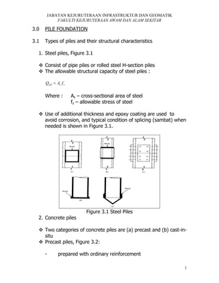
  • 1. JABATAN KEJURUTERAAN INFRASTRUKTUR DAN GEOMATIK FAKULTI KEJURUTERAAN AWAM DAN ALAM SEKITAR 3.0 PILE FOUNDATION 3.1 Types of piles and their structural characteristics 1. Steel piles, Figure 3.1  Consist of pipe piles or rolled steel H-section piles  The allowable structural capacity of steel piles : Qall  As f s Where : As – cross-sectional area of steel fs – allowable stress of steel  Use of additional thickness and epoxy coating are used to avoid corrosion, and typical condition of splicing (sambat) when needed is shown in Figure 3.1. Figure 3.1 Steel Piles 2. Concrete piles  Two categories of concrete piles are (a) precast and (b) cast-insitu  Precast piles, Figure 3.2: - prepared with ordinary reinforcement 1
  • 2. JABATAN KEJURUTERAAN INFRASTRUKTUR DAN GEOMATIK FAKULTI KEJURUTERAAN AWAM DAN ALAM SEKITAR - in the shape of square or octagonal Figure 3.2 Precast piles with ordinary reinforcement  Cast-in-situ or cast-in-place, Figure 3.3 : made by driving a steel casing with mandrel into the ground - - upon reaching the desired depth, mandrel is pulled out and the casing remain with or without pedestal uncased piles : - casing is driven to the desired depth, and filled with fresh concrete later gradually withdrawn - with or without pedestal allowable loads : cased pile : Qall  As f s  Ac f c uncased pile : Qall  Ac f c where : As – cross sectional area of steel Ac - cross sectional area of concrete fs – allowable stress of steel fc - allowable stress of concrete Figure 3.3 Cast in place concrete piles 2
  • 3. JABATAN KEJURUTERAAN INFRASTRUKTUR DAN GEOMATIK FAKULTI KEJURUTERAAN AWAM DAN ALAM SEKITAR 3. Timber piles  Three classifications are : o o o Class A : to carry heavy loads; min butt dia. = 14in (356mm) Class B : to carry medium loads; min butt dia. = 12-13in (305-330mm) Class C : used as temporary works but permanently for submerged structure; min butt dia. = 12in (305mm)  Splicing can be done by means of pipe sleeves or metal straps or bolts, Figure 3.4  The allowable load-carrying capacity : Qall  Ap f w Where : Ap – average cross-sectional area of the pile fw – allowable stress for the timber Figure 3.4 Splicing of timber piles (a) use of pipe sleeves (b) use of metal straps and bolts 4. Composite piles  Upper and lower portions of composite piles are made of different material  They may in the form of : steel-cast-in-place concrete or timber-concrete piles 3
  • 4. JABATAN KEJURUTERAAN INFRASTRUKTUR DAN GEOMATIK FAKULTI KEJURUTERAAN AWAM DAN ALAM SEKITAR 5. Pile in term of their function support capacity, Figure 3.5: (a) Bearing pile, (b) friction pile, (c) piles under uplift, (d) piles under lateral loads, (e) batter piles under lateral loads  Figure 3.5  Requirements and conditions for pile foundations, Figure 3.6 :  Figure 3.6 Conditions for use of pile foundations 4
  • 5. JABATAN KEJURUTERAAN INFRASTRUKTUR DAN GEOMATIK FAKULTI KEJURUTERAAN AWAM DAN ALAM SEKITAR - transmit load to the stronger underlying bedrock, 3.6(a) - gradually transmitting the load to the surrounding soil by means of frictional resistance at the soil-pile interface, 3.6(b) - subjected to horizontal load while supporting the vertical load transmitted by superstructure, 3.6(c) - built extended into hard stratum under collapsible soil (loess) to avoid the zone of moisture change that lead to swell and shrink, 3.6(d) - to resist uplifting forces for basement mats under water table, 3.6(e) - to resist scouring at the bridge abutments and piers that can lead to possible loss of bearing capacity of soil underneath, 3.6(f) 3.2 Estimating Pile Length, Figure 3.7 Figure 3.7 (a) and (b) Point Bearing Piles; and (c) Friction Piles  Length of pile estimation depending upon the mode of load transfer to the soil ; namely : o Point Bearing Piles - the ultimate capacity of the piles depends entirely on the bearing capacity of the hard stratum - hence the length, L of the pile is fairly well established 5
  • 6. JABATAN KEJURUTERAAN INFRASTRUKTUR DAN GEOMATIK FAKULTI KEJURUTERAAN AWAM DAN ALAM SEKITAR - the ultimate pile load is then; Qu  Q p  Qs (Figure 3.7a) where : Qp – load carried at the pile point Qs – load carried by skin friction developed at the side of the pile - piles can be extended into hard stratum with Qu  Q p (Figure 3.7b) o Friction Piles - if no hard stratum presence, piles are driven through softer soil to specified depths - resistance to vertical loading, is provided mainly by the skin friction; (in clayey soil is called adhesion) - the ultimate load is given by : Qu  Qs o Compaction Piles - piles are driven in granular soil to achieve proper compaction of soil close to ground surface - the length depends on :relative density before and after compaction as well as required depth of compaction 6
  • 7. JABATAN KEJURUTERAAN INFRASTRUKTUR DAN GEOMATIK FAKULTI KEJURUTERAAN AWAM DAN ALAM SEKITAR 3.3 Installation of Piles, Figure 3.8 Figure 3.8 Pile driving equipment  Four method used in piles driving are ; drop hammer, single acting air or steam hammer, double-acting and differential air or steam hammer, and diesel hammer - drop hammer, Figure 3.8a o raised by a winch, and allowed to drop at a certain height H o slow rate of hammer blows - single acting air or steam hammer, Figure 3.8b o ram is raised by air or steam pressure and then drops by gravity - double-acting and differential air or steam hammer, Figure 3.8c 7
  • 8. JABATAN KEJURUTERAAN INFRASTRUKTUR DAN GEOMATIK FAKULTI KEJURUTERAAN AWAM DAN ALAM SEKITAR o ram is raised and pushed downward by air or steam pressure - diesel hammer, Figure 3.8d o consist of ram, an anvil block and a fuel-injection system o ram is raised, fuel is injected near the anvil, ram is released, drops and compresses air-fuel mixture and ignites it o this causes; pile to be pushed downward and ram raised  Vibratory pile driver, Figure 3.8e; consists of counter-rotating weights that produces centrifugal force that cancel each other but sinusoidal dynamic vertical force produced pushes the pile downward 3.4 Pile Load Transfer Mechanism  Frictional resistance, f(z) with depth is given by : f z   Q z  pz  Where : Q z  - increase in pile load Δz – increase in depth P – perimeter of pile  Nature of variation of pile load is as given by Figure 3.9 and Woo and Juang(1970) has obtained actual variation of load transfer by a bored concrete pile in Taiwan as in Figure 3.10 8
  • 9. JABATAN KEJURUTERAAN INFRASTRUKTUR DAN GEOMATIK FAKULTI KEJURUTERAAN AWAM DAN ALAM SEKITAR Figure 3.9 Load transfer mechanism for piles 3.5 Figure 3.10 Load transfer curves for a concrete bored pile, Woo and Juang (1975) Equations for Estimating Pile Capacity  Ultimate load-carrying capacity of pile, Qu is : Qu  Q p  Qs Where : Qp – load-carrying capacity of the pile point Qs – frictional resistance  Point bearing capacity, Qp is : * * Q p  Ap q p  Ap cN c  q' N q  Where : Ap – cross sectional area of pile tip c – cohesion of the soil supporting the pile tip qp - unit point cohesion 9
  • 10. JABATAN KEJURUTERAAN INFRASTRUKTUR DAN GEOMATIK FAKULTI KEJURUTERAAN AWAM DAN ALAM SEKITAR q’ =γ’L – effective vertical stress at the level of the pile tip L- pile length * * N c , N q - the bearing capacity factors  Frictional resistance, Qs is : Qs   pLf Where : p – perimeter of the pile section ΔL – incremental pile length where, p and f is constant f – unit friction resistance at any depth z  There are many other methods for estimating Qp and Qs 3.6 Meyerhof’s Method – Estimation of Qp  The value of unit point resistance qp remains constant beyond the critical embedment ratio, (Lb/D)cr, Figure 3.11 Figure 3.11 Nature of variation of unit point resistance in a homogeneous sand  Figure 3.12 is the relationship of (Lb/D)cr and Ø(degree) where at Ø = 45°, (Lb/D)cr = 25 10
  • 11. JABATAN KEJURUTERAAN INFRASTRUKTUR DAN GEOMATIK FAKULTI KEJURUTERAAN AWAM DAN ALAM SEKITAR  For piles in sand, c=0; but Qp should not exceed Apql, * * Q p  Ap q p  Ap q' N q and Q p  Ap q' N q  Ap ql  The limiting point resistance is : SI unit : ql kN / m   50 N tan  ; or English 2 * q * ql lb / ft 2   1000 N q tan  * ql kip / ft 2   N q tan  Where : Ø – soil friction angle in the bearing stratum Figure 3.12 Nature of variation of unit point resistance in sand Figure 3.13 Variation of the maximum values of * N q with Ø  Using SPT method (Meyerhof, 1976): q p kN / m 2   40N L / D  400 N where N - average SPT number at 10D above and 4D below the pile point.  For piles in clay, with saturated and undrained conditions (Ø=0) * Q p  N c cu Ap  9cu Ap Where : cu – undrained cohesion (undrained shear strength) of the soil below the pile tip 11
  • 12. JABATAN KEJURUTERAAN INFRASTRUKTUR DAN GEOMATIK FAKULTI KEJURUTERAAN AWAM DAN ALAM SEKITAR 3.7 Vesic’s Method – Estimation of Qp  Vesic (1977) proposed value of Qp as : * ' * Q p  Ap q p  Ap cN c   o N  Where :  1  2K o  '  o - mean normal ground effective stress =  q '  3  Ko – earth pressure coefficient = 1 – sin Ø * N , N  - bearing capacity factors (see Table D.6 of Das textbook) * c 3.8 Janbu’s Method – Estimation of Qp NOT to be covered  Janbu (1976) proposed value of Qp as : * * Q p  Ap cN c  q' N q  Where : * * N c , N q - bearing capacity factors, Figure 9.14 Figure 3.14 (a)Meyerhof’s and (b) Janbu’s bearing capacity factors 12
  • 13. JABATAN KEJURUTERAAN INFRASTRUKTUR DAN GEOMATIK FAKULTI KEJURUTERAAN AWAM DAN ALAM SEKITAR 3.9 Coyle and Castello’s Method (Estimation of Qp in Sand) NOT TO BE COVERED  Coyle and Castello (1981) proposed value of Qp as : * Q p  q' N q Ap Where : q’ – effective vertical stress at the pile tip * N q - bearing capacity factor, Figure 3.15 13
  • 14. JABATAN KEJURUTERAAN INFRASTRUKTUR DAN GEOMATIK FAKULTI KEJURUTERAAN AWAM DAN ALAM SEKITAR * Figure 3.15 Variation of N q with L/D, unit frictional resistance and K value for piles in sand (Coyle and Castello, 1981) 3.10 Frictional Resistance, Qs in Sand  Frictional resistance is, Qs   pLf  Factors to be kept in mind while estimating unit frictional, f - the nature of pile installation unit skin friction increases with depth at similar depth, bored or jetted piles has a lower unit skin friction compared to driven piles  Approximation of f : (Figure 3.15) For z = 0 to L’ : For z = L’ to L : f  K v' tan  f  f z L' Where : K – effective earth coefficient  v' - effective vertical stress at specified depth  - soil-pile friction angle L’ = 15d  Read text for values of K, fav and Qs between 1976 and 1982 3.11 Frictional Resistance, Qs in Clay  Three method of estimating Qs in Clay : 1.  Method : - proposed by Vijayvergia and Focht (1972) - assumption : displacement of soil caused by pile driving results in a passive lateral pressure at any depth - average unit skin resistance as : 14
  • 15. JABATAN KEJURUTERAAN INFRASTRUKTUR DAN GEOMATIK FAKULTI KEJURUTERAAN AWAM DAN ALAM SEKITAR  ' f av    v  2cu  Where :  v' - mean effective vertical stress for entire embedment length,  A1  A2  A3  ...... L cu – mean undrained shear strength (Ø=0)  - refer to Figure 3.16b - total frictional resistance is : Qs  pLf av Figure 3.16a Critical embedment ratio and bearing capacity factors for various soil friction angles, (Meyerhof, 1976). 15
  • 16. JABATAN KEJURUTERAAN INFRASTRUKTUR DAN GEOMATIK FAKULTI KEJURUTERAAN AWAM DAN ALAM SEKITAR Figure 3.16b Variation of  with pile embedment length and its application, (McCleland – 1974). 2.  Method : - unit skin resistance in clayey soil is : f  cu  - empirical adhesion factor, Figure 3.17 α 16
  • 17. JABATAN KEJURUTERAAN INFRASTRUKTUR DAN GEOMATIK FAKULTI KEJURUTERAAN AWAM DAN ALAM SEKITAR Figure 3.17 Variation of  with undrained cohesion of clay - total frictional resistance is : Qs   fpL  cu pL 3.  Method : - assumption : excess pore water pressure in normally consolidated clay for driven pile shall dissipates gradually - thus unit frictional resistance for the pile is : f   v' Where :  v' - vertical effective stress = γ’z   K tan  R ØR – drained friction angle of remolded clay K – earth pressure coefficient Where : K  1 sin  R for normally consolidated clays K  1 sin  R  OCR for overly consolidated clays - total frictional resistance is : Qs   fpL 3.12 Point Bearing Capacity of Piles Resting on Rock  Goodman (1980) has approximate the ultimate unit point resistance in rock as : q p  qu N  1 Where : N  tan 2 45   / 2 qu – unconfined compression strength of rock  - drained angle of friction 17
  • 18. JABATAN KEJURUTERAAN INFRASTRUKTUR DAN GEOMATIK FAKULTI KEJURUTERAAN AWAM DAN ALAM SEKITAR  After taking care of scale effect, qu ( design)  qu (lab) 5  Table 3.1 is the typical value of qu(lab) for rocks and Table 3.2 the value of angle of friction respectively Table 3.1 Typical unconfined compressive strength of rocks qu lb/in2 MN/m2 10,000 – 20,000 15,000 – 30,000 5,000 – 10,000 20,000 – 30,000 8,500 – 10,000 Rock type Sandstone Limestone Shale Granite Marble 70 – 140 105 – 210 35 – 70 140 – 210 60 – 70 Table 3.2 Typical Values of angle of friction, Ø, of rocks Rock type Sandtone Limestone Shale Granite Marble Angle of friction, Ø 27 – 45 30 – 40 10 – 20 40 – 50 25 - 30  Hence, with FS = 3, the allowable point bearing capacity, Qp is : Q p ( all)  q u ( design) N    1 Ap FS Table 3.3 Typical pre-stressed concrete pile in use 18
  • 19. JABATAN KEJURUTERAAN INFRASTRUKTUR DAN GEOMATIK FAKULTI KEJURUTERAAN AWAM DAN ALAM SEKITAR Table 3.4 : Bearing capacity factors for deep foundations, N*c and N*σ, Vesic’s, 1977. 19
  • 20. JABATAN KEJURUTERAAN INFRASTRUKTUR DAN GEOMATIK FAKULTI KEJURUTERAAN AWAM DAN ALAM SEKITAR Table 3.5 Janbu’s bearing capacity factors 20
  • 21. JABATAN KEJURUTERAAN INFRASTRUKTUR DAN GEOMATIK FAKULTI KEJURUTERAAN AWAM DAN ALAM SEKITAR Example 3.1 Given : A square 305 mm x 305 mm concrete pile and 12 m long. Fully embedded in homogeneus sand layer, γd = 16.8 kN/m3 , c=0 and Øavg=35°. The average SPT value near pile tip is 16. Find : a. Qp using Meyerhof’s, Vesic’s, Janbu’s and SPT method. b. Qs using Qs   pLf and f  K v' tan  ..( for ..z  0  L' ) f  f z  L ' ...( for ...z  L'  L) if K=1.3 and   0.8 . c. Estimate the load-carrying capacity of pile, Qall if FS=4. d. Qall using Coyle and Costello’s method Solution : a. Meyerhof’s : Because it is a homogeneous soil, Lb=L. For Ø=35°, (Lb/D)cr =(L/D)cr ≈ 10 (Figure 3-16a). So for this pile, Lb/D = 39.34 > * (Lb/D)cr. Hence, from the same figure N q  120 * Q p  Ap q p  Ap q' N q  0.0929201.6120  2247.4kN * ql kN / m 2   50 N q tan   50120tan 35  4201.25kN / m 2 * Q p  Ap ql  0.09294201  390.3kN  Ap q' N q Qp = 390 kN * Vesic’s : use I rr  90 ; with Ø=35°; N  79.5 so : 1  21  sin   ' * * Q p  A p o N   A p   q' N  3   1  21  sin 35  0.0929  201.679.5  923kN 3   * Janbu’s : with c=0; use  '  90;..and ..  35;..N q  41.3 by int erpolation  * Q p  Ap q' N q  0.0929m 2 201.6kN / m 2 41.3  773.5kN SPT method : q p kN / m 2   40N L / D  400 N Q p  Ap q p  0.0929m 2 401639.34  2339kN 21
  • 22. JABATAN KEJURUTERAAN INFRASTRUKTUR DAN GEOMATIK FAKULTI KEJURUTERAAN AWAM DAN ALAM SEKITAR Limiting value = Q p  Ap 400 N  0.0929m 2 40016  595kN For design purpose : Q p  595kN  773.5kN  390kN  586kN 3 b. from sub-topic 3.10 from the note : L'  15D  150.305m  4.58m For z = 0 :  v'  0; f  K v' tan   0 For z = L’ to L :  v'  L'  16.8kN / m 3 4.58m  76.94kN / m 2 f  K v' tan   1.376.94tan0.8  35  53.2kN / m 2 Thus  f  f z  4.58m  Qs   z  0  pL' f z  20 ft pL  L' 2   2  0  53.2kN / m  4  0.305m 4.58m   53.2kN / m 2 4  0.305m 12  4.58m  :    2      149  482  631kN c. thus load carrying capacity of pile, Qu = Qp(avg) + Qs Q p ( avg )  586kN and Qs  631kN;.....Qall  Qult 586  631   304.25kN FS 4 d. Coyle and Castello’s * Qult  Q p  Qs  q' N q Ap  K v' tan0.8  pL;....and ... L 12   39.3 D 0.305 * For Ø=35° and L/D=39.3; N q  40 K≈1.0 Thus : * Qult  Q p  Qs  q' N q A p  K v' tan0.8  pL      201.6kN / m 2 40  0.0929m 2  1.016.8  12  tan0.8  354  0.30512   749  1569  2318kN And Qall  Qult 2318   579.6kN FS 4 22
  • 23. JABATAN KEJURUTERAAN INFRASTRUKTUR DAN GEOMATIK FAKULTI KEJURUTERAAN AWAM DAN ALAM SEKITAR Example 3.2 Given : A driven pile in clay as in Figure E9.2. The pipe pile has outside diameter of 406mm and wall thickness of 6.35mm. Find : a. Net point bearing capacity. b. Skin resistance using α, λ and β method if ØR =30°; the top 10m is normally consolidated clay and the bottom clay layer has OCR=2. c. Net allowable pile capacity, Qall if FS=4. Solution : a. Cross section of pile, Ap   D2   0.4062  0.1295m 2 4 4 * Q p  Ap q p  Ap N c cu ( 2)  0.12959100  116.55kN b. Skin resistance, Qs : (α method) : Qs   fpL  cu pL From Figure α vs cu : cu(1)=30kN/m2 α=1.0; cu(2)=100 α=0.5 Thus : Qs   fpL   cu pL   1cu (1)  0.40610   2 cu ( 2)  0.40620  130 0.40610  0.5100 0.40620  1658.2kN (λ method) : where f av    v'  2cu ( av)  cu ( avg )  cu (1) 10  cu ( 2) 20 30  3010  10020  76.7kN / m 2 30 Use the plotted Figure E9.2b, for σ’v vs depth; ' v  A1  A2  A3 225  552.38  4577   178.48kN / m 2 L 30 23
  • 24. JABATAN KEJURUTERAAN INFRASTRUKTUR DAN GEOMATIK FAKULTI KEJURUTERAAN AWAM DAN ALAM SEKITAR From Figure λ vs L; λ=0.14 for L=30m; so f av    v'  2cu ( av)   0.14178.48  276.7  46.46kN / m 2 Hence; Qs  pLf av   0.4063046.46  1777.8kN (β method) : where ØR =30°; f   v' ;   K tan  R ; K  1 sin  R K  1 sin  R  OCR For z=0-5m :  0  90  2 f av(1)  1  sin  R  tan  R v' ( av)  1  sin 30tan 30   13.0kN / m 2   For z=5-10m :  90  130.95  2 f av( 2)  1  sin  R  tan  R v' ( av)  1  sin 30tan 30   31.9kN / m 2   For z=10m-30m , OCR=2:  130.95  326.75  2 f av(3)  1  sin  R  tan  R OCR v' ( av)  (1  sin 30)tan 30 2    93.43kN / m 2   so   Qs  p f av(1) 5  f av( 2) 5  f av(3) 20   0.406135  31.95  93.4320  2669.7kN c. So use α and λ method which produced almost similar results, Qs  1658.1  1777.8  1718kN 2 Qult  Q p  Qs  116.46  1718  1834.46kN;....hence...Qall  Qult 1834.46   458.6kN FS 4 Example 3.3 Given : An H-pile (size HP 310 x 1.226), length of embedment = 26m, driven through soft clay and rest on sandstone, qu(lab) for sandstone = 76 MN/m2, Ø=28°, FS=5. Find : The allowable point bearing capacity, Qp(all) Solution : Since q p  qu N  1 ; N  tan 2 45   / 2 and qu ( design)  qu (lab) 5       qu ( lab)   2   tan  45    1  A p 5  2 q p Ap qu N   1A p      Q p ( all )     FS FS FS  76  10 3 kN / m 2    28  2 3 2   1  15.9  10 m    tan  45  5 2          182kN 5   24
  • 25. JABATAN KEJURUTERAAN INFRASTRUKTUR DAN GEOMATIK FAKULTI KEJURUTERAAN AWAM DAN ALAM SEKITAR EXAMPLE OF FINAL EXAMINATION QUESTION Q4 The most common function of piles is to transfer a load that cannot be adequately supported at shallow depths to a depth where adequate support becomes available. Hence, the piles can also be categorized based on its function/ support capacity. (a) Briefly describe with relevant sketches the five (5) functions / support capacity of piles. (5 marks) (b) Reinforced concrete piles 18 m long, of square section and width 400 mm are driven through 8 m of loose fill with unit weight of 13 kN/m3 to penetrate 10 m into an underlying firm to stiff saturated clay. The groundwater table is found at a depth of 2 m below ground surface. (i) Determine the ultimate bearing capacity, Qult, of pile by the given formula, if the undrained shear strength of the clay increases linearly with depth from 65 kN/m2 at the top of the clay to 100 kN/m2 at a depth of 10 m below the surface of the clay. Assuming that the unit weight of stiff saturated clay is 17 kN/m3 throughout the layer and the frictional capacity of the loose fill is negligible. (10 marks) (ii) Assuming that it is necessary to provide a number of such piles to carry the total foundation load, explain the bearing capacity of the pile group is estimated? Discuss your answer with the help of relevant sketches. (5 marks) 25
  • 26. JABATAN KEJURUTERAAN INFRASTRUKTUR DAN GEOMATIK FAKULTI KEJURUTERAAN AWAM DAN ALAM SEKITAR ANSWER Q4 The most common function of piles is to transfer a load that cannot be adequately supported at shallow depths to a depth where adequate support becomes available. Hence, the piles can also be categorized based on its function/ support capacity. (a) Briefly describe with a relevant sketch what are the five (5) function/ support capacity of piles. (5 marks) (a) Bearing pile, (b) friction pile, (c) piles under uplift, (d) piles under lateral loads, (e) batter piles under lateral loads (b) A reinforced concrete piles 18 m long, of square section and width 400 mm is driven through 8 m of loose fill with unit weight of 13 kN/m3 to penetrate 10 m into the underlying firm to stiff saturated clay. The groundwater table is found at a depth of 2 m below ground surface. (i) Determine the ultimate bearing capacity, Qult of pile by the given formula, if the undrained shear strength of the clay increases 26
  • 27. JABATAN KEJURUTERAAN INFRASTRUKTUR DAN GEOMATIK FAKULTI KEJURUTERAAN AWAM DAN ALAM SEKITAR linearly with depth from 65 kN/m2 at the top of the clay to 100 kN/m2 at a depth of 10 m below the surface of the clay. Assuming that the unit weight of firm to stiff saturated clay is 17 kN/m3 throughout the layer and the frictional capacity of the loose fill is negligible. Given that:-   qtip = cu Nc (Based on Meyerhof’s equation); f s ( avg )    v '  2cu (10 marks) Answer:To determine Qp:qtip = cu Nc = 100 kN/m2 x 9 = 900 kN/m2 [1M] Ap = 0.4 x 0.4 = 0.16 m2 [1M] Qp = Apqtip = 0.16 x 900 = 144 kN [0.5M] To determine Qs:- (45.14  117.04)(10) 2 v'   81.09kN / m 2 10 Elevation (m) 0 2 8 18 [1M] Effective Vertical Pressure (kN/m2) 0 26 45.14 117.04 [1M] (65  100)(10) 2 cu   82.5kN / m 2 10 Based on Figure 1,  = 0.185  [1M] [1M]  f s ( avg )    v '  2cu = (0.185)[81.09+2(82.5)] = 45.53kN/m2 As = 4 x 0.4 x 10 = 16 m2 [1M] [0.5 M] 27
  • 28. JABATAN KEJURUTERAAN INFRASTRUKTUR DAN GEOMATIK FAKULTI KEJURUTERAAN AWAM DAN ALAM SEKITAR Qs = As. fs = 16 x 45.53 = 728.48 kN [1M] Qult = Qs + Qp = 728.48 + 144 = 872.48 kN [1M] (ii) Assuming that it is necessary to provide a number of such piles to carry the total foundation load, how could the bearing capacity of the pile group be estimated? Discuss your answer with a relevant sketch. (5 marks) Answer:For most practical purposes, the ultimate load of pile group, (QvG)ult, can be estimated based on the smaller value of the following two values:(a) Group Action – block failure (Figure A) of pile group by breaking into the ground along an imaginary perimeter and bearing at the base. The ultimate capacity for the group failure can be estimated from the following relationship:(QvG)ult =  x n x (Qv)ult [2M] (b) Individual Action (Figure B) – if there is no group action (when the center to center spacing, s, is large enough, >1), in that case, the piles will behave as individual piles. The total load of the group can be taken as n times the load of the single pile, in which (QvG)ult = n x (Qv)ult =  (Qv)ult [2M] 28
  • 29. JABATAN KEJURUTERAAN INFRASTRUKTUR DAN GEOMATIK FAKULTI KEJURUTERAAN AWAM DAN ALAM SEKITAR Figure : (A) Individual action, (B) Group action [2 x 0.5M = 1M 3.13 Pile Load Test  Pile load test arrangement by means of hydraulic jack is shown in Figure 3.18a  Step loads are applied to the pile, so that a small amount of settlement is allowed to occur  Settlement from field test is recorded as in Figure 3.18b  Net settlement calculation for any load Q : - When Q = Q1 : Net settlement, snet(1)  st (1)  se(1) 29
  • 30. JABATAN KEJURUTERAAN INFRASTRUKTUR DAN GEOMATIK FAKULTI KEJURUTERAAN AWAM DAN ALAM SEKITAR - When Q = Q2 : Net settlement, snet( 2)  st ( 2)  se( 2) Where : snet – net settlement se – elastic settlement of the pile itself st – total settlement  The values of Q then plotted against se produces diagram in Figure 3.18c Figure 3.18 (a) Test arrangement (b) load vs total settlement (c) load vs net settlement 3.14 Failure criteria of a pile  The ultimate failure load for a pile is defined as the load when the pile plunges or the settlements occur rapidly under sustained load and the amount of settlement exceed the acceptable soil-pile system  Or  Besides it, many engineers define the failure load at the point of intersection of the initial tangent to the load-settlement curve and the tangent to or the extension of the final portion of the curve. 30
  • 31. JABATAN KEJURUTERAAN INFRASTRUKTUR DAN GEOMATIK FAKULTI KEJURUTERAAN AWAM DAN ALAM SEKITAR  Arbitrary settlement limits that the pile is considered to have failed when the pile head has moved 10 percent of the pile end diameter or the gross settlement of 1.5 in. (38 mm) and net settlement of 0.75 in. (19 mm) occurs under two times the design load. (JKR standard)   However, all of these definitions for defining failure are judgemental. 3.15 Pile Driving Formulas  Due to varying soil profiles layers a point bearing pile cannot always satisfied the capability of penetrating the dense soil to a predetermined depth; therefore several equations have been developed by many to calculate the ultimate capacity of pile during driving.  According to Engineering News Record (ENR), Qu is : Qu  WR h S C Where : WR – weight of the ram h – height of fall of the ram S – penetration of pile per hammer blow (from last few driving blows) C – a constant (for drop hammers : C = 1 in. ; S and h are in inches) (for steam hammers : C = 0.1 in. ; S and h are in inches) FS = 6 For single and double-acting hammers WRh is replaced by EHE Thus : Qu  EH E S C Example 3.4 A precast concrete pile 12 in. x 12 in. in cross section is driven by a hammer. Given : Maximum rated hammer energy = 30 kip-ft Hammer efficiency = 0.8 31
  • 32. JABATAN KEJURUTERAAN INFRASTRUKTUR DAN GEOMATIK FAKULTI KEJURUTERAAN AWAM DAN ALAM SEKITAR Weight of ram = 7.5 kip Pile length = 80 ft Coefficient of restitution = 0.4 Weight of pile cap = 550 lb Ep = 3 x 10⁶ kip/in2 Number of blows for last 1 in. of penetration = 8 Estimate the allowable pile capacity by the a. Modified ENR formula (use FS=6) b. Danish formula (use FS = 4) c. Gates formula (use FS = 3) Solution : a. Weight of pile + cap = 12  12  80150lb / ft 3   550  12.55kip 12 12 and WR h  30kip  ft 2 EW R h WR  n W p 0.830  12kip  in  7.5  0.42 12.55 Qu    607kip 1 S  C WR  W p 7.5  12.55 8  0.1 Qall  b. Qu 607   101kip FS 6 EH E Qu  EH E L S 2 Ap E p Use Ep = 3 x 10⁶ lb/in2 And Qu  Qall c. EH E L  2 Ap E p 0.830  1280  12  3  10 6  212  12 kip / in 2   1000     0.566in. 0.830  12  417kip  0.566 417   104kip 4 1 8 Qu  a EH E b  log S   27 0.8301  log1   252kip 8 252 Qall   84kip 3 3.16 Hiley’s Formula for estimating single RC pile capacity. 32
  • 33. JABATAN KEJURUTERAAN INFRASTRUKTUR DAN GEOMATIK FAKULTI KEJURUTERAAN AWAM DAN ALAM SEKITAR The Hiley’s formula gives the simplest method of calculating the final setting or the ultimate load of a pile while driving depending upon the given parameter. It is usually written as : BW H h WH  Pe 2 C s   2 FS  WL WH  P And C  Cc  C p  C q where : s C WH h P P1 P2 WL FS e Cc - Set value /1 blow (mm/blow) - Temporary compression of pile & soil (mm) - Weight of hammer (kN) - Drop of hammer (mm) - Total load (P1 + P2) (kN) - Weight of pile (kN) - Weight of driving assembly (kN) - Pile working load (kN) - Factor of safety - Coefficient of restitution - Temporary compression coefficient due to pile head and cap (mm), Table 3.3 Cp, - Temporary compression coefficient due to pile length (mm), Table 3.3 Cq, - Temporary compression coefficient due to ground or quake (mm), Table 3.3 Note : (a) (b) (c) (d) This formula was developed by Hiley (1925). The formula assumes the energy of the falling hammer during pile driving is proportional resisted by the pile. This method is widely considered to be one of the better formulas that intended to be applied to cohesionless, well-drained soils or rock. Weight of the hammer shall be about 0.5 to 2.0 times of the total pile weight. The term mass and weight are interchangeably The term Cp and Cq are shown in Figure 3.19 after a pile set measurement of pile are made. 33
  • 34. JABATAN KEJURUTERAAN INFRASTRUKTUR DAN GEOMATIK FAKULTI KEJURUTERAAN AWAM DAN ALAM SEKITAR Figure 3.19 : Example graph of pile set Table 3.6 : Values of Cc, Cp and Cq Form of compression Pile head and cap, Cc Pile length, Cp Quake, Cq Material Head of timber pile Short dolly in helmet or driving cap 3 in/76.2mm packing under helmet or driving cap 1 in/25.4mm pad only on head of reinforced concrete pile Timber pile (E=1,500,000 lb/in2) or (E=10,342,500 kPa) Pre-cast pile (E=2,000,000 lb/in2) or (E=13,790,000 kPa) Steel pile for cast in place (E=30,000,000 lb/in2) or (E=206,850,000 kPa) Ground surrounding pile and under pile Easy driving (inch) Medium driving (inch) Hard driving (inch) Very hard driving (inch) 0.05 0.10 0.15 0.20 0.05 0.10 0.15 0.20 0.07 0.15 0.22 0.30 0.03 0.05 0.07 0.10 0.004L 0.008L 0.012L 0.016L 0.003L 0.006L 0.009L 0.012 0.003L 0.006L 0.009L 0.012 0.05 0.10 – 0.20 0.15 – 0.25 0.05 – 0.15 34
  • 35. JABATAN KEJURUTERAAN INFRASTRUKTUR DAN GEOMATIK FAKULTI KEJURUTERAAN AWAM DAN ALAM SEKITAR point Note : Length, L measure in feet 1 feet = 0.3048 m 1 inch = 25.4 mm Table 3.7 : Coefficient of restitution, e. Description Coefficient of restitution, e Piles driven with double acting hammer - Steel piles without driving cap Reinforced concrete pile without helmet but with packing on top of pile Reinforced concrete piles with short dolly in helmet and packing Timber pile 0.5 0.5 0.4 0.4 Piles driven with single acting and drop hammer - Reinforced concrete piles without helmet but with packing on top of piles Steel piles or steel tube of cast in place piles fitted with driving cap and short dolly covered by steel plate Reinforced concrete piles with helmet and packing, dolly in good condition Timber pile in good condition Timber pile in poor condition 0.4 0.32 0.25 0.25 0.00 Example 3.5 Using Hiley’s formula calculate the final set of a 200mm X 200mm RC pile. The pile driven with single acting and drop hammer with medium driving. The type of pile is the reinforced concrete pile with helmet and packing, dolly in good condition. Other data and parameters are : Pile working load, Mass of hammer, Factor of safety, FS Pile length, L Mass driving assembly, Drop of hammer, Hammer efficiency, = 275 kN = 25 kN = 2.0 = 18 m = 2.0 kN = 400 mm = 85% 35
  • 36. JABATAN KEJURUTERAAN INFRASTRUKTUR DAN GEOMATIK FAKULTI KEJURUTERAAN AWAM DAN ALAM SEKITAR Density of concrete, = 24 kN/m3 Solution : Mass of pile, P1 = Concrete density X Area X Length of pile = 24 X (0.2 X 0.2) X 18 = 17.28 kN Total load, P = P1 + P2 = 17.28 + 2.0 = 19.28 kN Value of e = 0.25 (Table 3.7) BW H h 0.8525400  15.454mm  FS  WL 2.0  275 WH  Pe 2 25  19.28  0.252   0.592 WH  P 25  19.28 Value of C Cc Cp Cq : = 0.15in X 25.4 = 3.81 mm = 0.006(59ft) = 0.354in X 25.4 = 8.99 mm = 0.10in X 25.4 = 2.54 mm C = Cc + Cp + Cq = 3.81 + 8.99 + 2.54 = 15.34 mm BW H h WH  Pe 2 C s   2 FS  WL WH  P 15.34  15.454  0.592 2  s  1.48mm / blow  or S  14.8mm / 10blow ( Final Set ) Using  s  Example 3.6 Given : 36
  • 37. JABATAN KEJURUTERAAN INFRASTRUKTUR DAN GEOMATIK FAKULTI KEJURUTERAAN AWAM DAN ALAM SEKITAR A 200mm x 200mm RC square pile. The pile driven with single-acting and drop hammer with hard driving. The type of pile is reinforced concrete pile with helmet and packing, dolly in good condition. Mass of hammer, Wn Factor of safety, FS Pile length, l Mass Driving assembly,P2 Drop hammer, h Hammer efficiency, B Set value, S =25kN =2.0 =24m =3.0 kN =500mm =85% =19mm/10 blow (Figure 3.20) Figure 3.20 Required : Ultimate load of pile Solution : Mass of pile, P1 = Concrete densityxAreaxlength = 24x(0.2x0.2)x24=23.04kN Total load, P2 Value of e Cp + Cq Cc Temporary compression, C Set value, s = = = = P1 + P2 = 23.04 + 3=26.04kN 0.25 (Table 3.7) 20mm (Figure 3.20) 0.22inx25.4=5.59mm = 5.59 + 20 = 25.59mm = 19mm/10 blow =1.9mm/blow 37
  • 38. JABATAN KEJURUTERAAN INFRASTRUKTUR DAN GEOMATIK FAKULTI KEJURUTERAAN AWAM DAN ALAM SEKITAR BW H h  0.8525500 1  1    FS  s  C c  C p  C q  2.01.9  25.59 2  2    2 2 WH  Pe 25  26.040.25   0.5217 WH  P 25  26.04  361.52kN By using Hiley’s equation : WL  WH  Pe 2  361.52  0.5217  188.6kN  1  WH  P FS  s  C p  C q  C c   2  BW H h  Therefore, the pile working load must be less than 188.6kN 3.17 Settlement of Piles, Vesics (1969)  Settlement of a pile under vertical working load, Qw is : s  s1  s 2  s3 Where : s – total pile settlement s1 – elastic settlement of pile s2 – settlement caused by the load at the pile tip s3 – settlement caused by the load transmitted along pile shaft  Formulae : - elastic settlement, s1 : s1  Q wp  Qws L Ap E p Where : Qwp – load carried at the pile point under working condition Qws – load carried by frictional resistance under work load Ap – area of pile cross section L – length of pile Ep – modulus of elasticity of the pile material  - nature of unit skin friction (=0.5 or 0.67), Figure 3.21 38
  • 39. JABATAN KEJURUTERAAN INFRASTRUKTUR DAN GEOMATIK FAKULTI KEJURUTERAAN AWAM DAN ALAM SEKITAR Figure 3.21 Various types of unit friction resistance along pile shaft - load at pile point, s2 : s2  q wp D Es 1   I 2 s wp Where : D – width or diameter of pile qwp – point load per unit area = Qwp/Ap Es – modulus of elasticity of soil at or below the pile point μs – Poisson’s ratio of soil Iwp – influence factor = 0.85 Or s2  Qwp C p Dq p Where : qp – ultimate point resistance of the pile Cp – an empirical coefficient, Table 3.8 Table 3.8 Typical Values of Cp Soil type Sand (dense to loose) Clay (stiff to soft) Silt (dense to loose) Driven Pile 0.02-0.04 0.02-0.03 0.03-0.05 Bored Pile 0.09-0.18 0.03-0.06 0.09-0.12 - load carried by pile shaft, s3 : Q  D 2 s3   ws   pL  E 1   s I ws   s   Where : 39
  • 40. JABATAN KEJURUTERAAN INFRASTRUKTUR DAN GEOMATIK FAKULTI KEJURUTERAAN AWAM DAN ALAM SEKITAR p – perimeter of the pile L – embedded length of pile Iws – influence factor = 2  0.35 Or s3  L D and Cs (a constant) = 0.93  0.16 L / D C p Qws C s Lq p Cp from Table 3.8 Example 3.7 Given : A pre-stressed concrete pile 21m long, being driven into sand. Working load, Qw = 502 kN. The pile is octagonal in shape with D = 356 mm, see Figure E9.4. Skin resistance, Qs carries 350 kN, and Qp carries the rest. Use Ep = 21 x 106 kN/m2, Es = 25 x 103 kN/m2, μs = 0.35 and ξ = 0.62. Find : The settlement of the pile. Solution : From Table D3; for D=356mm, Ap=1045cm2, p=1.168mm and Qws=350 kN; so Qwp=502-350=152 kN Due to material : s1  Q  Qws L wp Ap E p  152  0.6235021  0.00353m  3.35mm  0.1045m 2 21  10 6  q wp  Qwp Ap Due to point load : s2  q wp D Es 1   I 2 s wp    152  0.356   1  0.35 2 0.85  0.0155m  15.5mm  3   0.1045  25  10  Due to skin : With I ws  2  0.35 L 21  2  0.35  4.69 D 0.356 40
  • 41. JABATAN KEJURUTERAAN INFRASTRUKTUR DAN GEOMATIK FAKULTI KEJURUTERAAN AWAM DAN ALAM SEKITAR Q  D  350  0.356  2 2 s3   ws   pL  E 1   s I ws  1.16821 25  10 3  1  0.35 4.69 And      s  0.00084mm  0.84mm     Therefore the total settlement is : s  s1  s2  s3  3.35  15.5  0.84  19.69mm 3.18 Pullout Resistance of Piles  The gross ultimate resistance of a pile subjected to uplifting force, Figure 3.22 is : Tug  Tun  W Where : Tug – gross uplift capacity Tun – net uplift capacity W – effective weight of pile Figure 3.22 Uplift capacity of piles a. In Clay  Das and Seeley (1982), estimated Tun as : 41
  • 42. JABATAN KEJURUTERAAN INFRASTRUKTUR DAN GEOMATIK FAKULTI KEJURUTERAAN AWAM DAN ALAM SEKITAR Tun  Lp ' cu Where : L – length of the pile p – perimeter of pile section  ’- adhesion coefficient at soil-pile interface cu – undrained cohesion of clay Values of  ' :  - for cast-in-situ: (for bore pile) 2  '  0.9  0.00625cu for cu ≤ 80 kN/m 2  ' 0.4 for cu > 80kN/m - for pipe piles :  '  0.715  0.0191cu for cu ≤ 27 kN/m  ' 0.2 for cu > 27 kN/m 2 2 b. In Sand Das and Seeley (1975), estimated Tun as :  Tun   L 0  f u p dz with fu varies by f u  K u v' tan  for (z≤Lcr) such as in Figure 3.23a  - Steps in finding Tun in dry soil; find relative density and use Fig 3.23c to find Lcr if L ≤ Lcr then : Tun  1 pL2 K u tan  with values Ku and  from Figure 2 3.23b&c - if L > Lcr then : 42
  • 43. JABATAN KEJURUTERAAN INFRASTRUKTUR DAN GEOMATIK FAKULTI KEJURUTERAAN AWAM DAN ALAM SEKITAR Tun  1 pL2 K u tan   pLcr K u tan  L  Lcr  with values Ku and cr 2  from Figure 3.23b&c Where : Ku – uplift coefficient  v' - effective vertical stress at a depth z  - soil-pile friction  Thus with FS=2 to 3, allowable uplift capacity Tu(all) is : Tu ( all)  Tug FS Figure 3.23 (a) Variation of fu (b) Ku (c) Variation of  /Ø, (L/D)cr with relative density of sand Dr Example 3.8 43
  • 44. JABATAN KEJURUTERAAN INFRASTRUKTUR DAN GEOMATIK FAKULTI KEJURUTERAAN AWAM DAN ALAM SEKITAR Given : A 50 ft long concrete pile embedded in a saturated clay cu=850 lb/ft2. 12 in x 12 in. in cross section. Use FS=4. Find : Allowable pullout capacity, Tun(all) Solution : with cu =850 lb/ft2 ≈ 40.73 kN/m2  '  0.9  0.00625cu   0.9  0.0062540.73  0.645 504  10.645850  109.7kip 1000 109.7 109.7    27.4kip FS 4 Tun  Lp ' cu  And Tun( all) Example 3.9 Given : A precast concrete pile, with cross section = 350mm x 350mm. Length of pile as 15m. Assume : γsand=15.8 kN/m3, Øsand=35°, Dr=70%. Find : Pullout capacity if FS=4. Solution : From Figure 3.23; for Ø=35° and Dr=70% L    14.5;..Lcr  14.50.35m   5.08m  D  cr   1;..  135  35;.......K u  2  Hence : for L (15m) > Lcr (5.08m) Tun  1 pL2 K u tan   pLcr K u tan  L  Lcr  cr 2  1 2 0.35  415.85.082 2 tan 35  0.35  415.85.08215  5.08 tan 35  1961kN Tu ( all)  Tug FS  1961  490kN 4 44
  • 45. JABATAN KEJURUTERAAN INFRASTRUKTUR DAN GEOMATIK FAKULTI KEJURUTERAAN AWAM DAN ALAM SEKITAR 3.19 Group piles efficiency  Converse –Labarre method of estimating pile-group efficiency developed by Jumikis, 1971 using the following equation : Eg  1   n  1m  m  1n 90mn Where : Eg – pile-group efficiency θ – tan-1(d/s), (deg) n – number of piles in row m – number of rows of piles d – diameter of piles s – spacing of piles, center to center, same unit as pile diameter. Example 3.10 Given : A pile group consists of 12 friction piles in cohesive soil, Figure 3.24. Each pies diameter is 300mm and center-to-center spacing is 1 m. By means of a load test, the ultimate load of a single pile was found to be 450 kN. Take SF as 2.0. Required : Design capacity of the pile group, using the Converse-Labarre equation. 1  3   tan 1    18.4 ; E g  1  18.4 4  13  3  14  0.710 9034 Allowable bearing capacity of a single pile=450kN/2=225kN Design capacity of the pile group = 0.710(12)(225kN)=1917kN. 45
  • 46. JABATAN KEJURUTERAAN INFRASTRUKTUR DAN GEOMATIK FAKULTI KEJURUTERAAN AWAM DAN ALAM SEKITAR Figure 3.24  Another method of estimating efficiency of pile group as quoted by Das (2007) as follows :  A pile cap is normally constructed over group piles; either in contact or well above the ground, Figure 3.25 a&b.  In practice, minimum center-to-center pile spacing, d = 2.5D, or 3-3.5D as in ordinary situations; where D - diameter of piles  Thus, the efficiency of a group pile, η is :  Qg (u ) Q u Where : Qg(u) – ultimate load-bearing capacity of the group pile Qu – ultimate load-bearing capacity of each pile without group effect  If group as a block thus :  2n1  n2  2d  4d pn1 n2 46
  • 47. JABATAN KEJURUTERAAN INFRASTRUKTUR DAN GEOMATIK FAKULTI KEJURUTERAAN AWAM DAN ALAM SEKITAR Figure 3.25 Pile groups 3.26 timate Capacity of Group Piles in Saturated Clay  For most practical purposes, the ultimate load of pile group, (QvG)ult, can be estimated based on the smaller value of the following two values, Figure 3.27 (a) and (b):(a) Group Action – block failure (Figure A) of pile group by breaking into the ground along an imaginary perimeter and bearing at the base. The ultimate capacity for the group failure can be estimated from the following relationship:(QvG)ult =  x n x (Qv)ult (b) Individual Action (Figure B) – if there is no group action (when the center to center spacing, s, is large enough, >1), in that case, the piles will behave as individual piles. The total load of the group can be taken as n times the load of the single pile, in which (QvG)ult = n x (Qv)ult =  (Qv)ult 47
  • 48. JABATAN KEJURUTERAAN INFRASTRUKTUR DAN GEOMATIK FAKULTI KEJURUTERAAN AWAM DAN ALAM SEKITAR Figure 3.27 : (A) Individual action, (B) Group action  Feld’s Method : in estimating group capacity of friction piles, Qg(u) Figure 3.28 Feld’s Method Table 3.9 Arrangement of Feld’s Method Pile type A B C No. of Piles 1 4 4 No. of adjacent piles 8 5 3 Reduction factor for each pile 1-8/16 # 1-5/16 1-3/16 Note: 16 # no. of arrow Ultimate capacity Col.2 x Col.4 0.5Qu 2.75Qu 3.25Qu Σ6.5Qu=Qg(u) 48
  • 49. JABATAN KEJURUTERAAN INFRASTRUKTUR DAN GEOMATIK FAKULTI KEJURUTERAAN AWAM DAN ALAM SEKITAR  Therefore, efficiency,   Qg (u ) Q  u 6.5Qu  72% 9Qu 3.20 Ultimate Capacity of Group Piles in Saturated Clay  Figure 3.29 shows a group of pile in saturated clay, steps to find the ultimate load-bearing capacity Qg(u) are : Find Qu in pile group :  As individual From :  Qu  n1n2 Q p  Qs ; Q p  Ap 9cu ( p)  and Qs  pcu L So Q : u   n1n2 9 Ap cu ( p )  pcu L  (1)  As pile group (dimensions of LgxBgxL): p c L   2Lg  Bg cu L g u  Point bearing capacity as : Ap q p  Ap cu ( p ) N c*  Lg Bg cu ( p ) N c*  With N c* from Figure 3.29, thus : Q u *  Lg Bg cu ( p ) N c   2Lg  Bg cu L (2) Where : D D Lg  n1  1d  2  and Bg  n2  1d  2  2 2  The lower value from (1) and (2) is Qg(u) 49
  • 50. JABATAN KEJURUTERAAN INFRASTRUKTUR DAN GEOMATIK FAKULTI KEJURUTERAAN AWAM DAN ALAM SEKITAR Figure 3.29 Ultimate group piles in clay Figure 3.30 Variation of N c* with Lg/Bg and L/Bg 50
  • 51. JABATAN KEJURUTERAAN INFRASTRUKTUR DAN GEOMATIK FAKULTI KEJURUTERAAN AWAM DAN ALAM SEKITAR Example 3.11 Given : The section of 3 x 4 group pile in a layered saturated clay is shown in Figure 3.31. The piles are square in cross section (350mm x 350mm). The center-to-center spacing d, of the piles is 1220mm. Required : The allowable load-bearing capacity of the pile group. Use FS=4. 5m 40 kN/m2 10 m 70 kN/m2 1.22 m Figure 3.31 Group pile in clay soil If pile act as single pile: Q u   n1 n2 9 Ap cu ( p )   pcu L    n1 n2 9 Ap cu ( p )   1 pcu (1) L1   2 pcu ( 2) L2 2  2 With cu(1)=40 kN/m ;α1=0.86 and cu(2)=70 kN/m ;α2=0.63 thus; Ap=0.350x0.350=0.093m2, p=4x0.350=1.22m Q u  n1 n2 9 A p cu ( p )   1 pcu (1) L1   2 pcu ( 2) L2   3  490.09370  0.861.22405  0.631.227010  3  458.6  209.8  538.02  9677.04kN If pile as a group : D Lg  n1  1d  2   4  11.22  0.305  3.965m 2 D Bg  n2  1d  2   3  11.22  0.305  2.745m 2 51
  • 52. JABATAN KEJURUTERAAN INFRASTRUKTUR DAN GEOMATIK FAKULTI KEJURUTERAAN AWAM DAN ALAM SEKITAR Lg Bg  3.965 L 15  1.44;.....   5.46 2.745 Bg 2.745 From Figure 3.29: N c*  8.6 (assuming : that at the end of curve at right hand stays horizontal) Thus : Q u *  Lg Bg cu ( p ) N c   2Lg  Bg cu L  3.9652.745708.6  23.965  2.745405  7010  6552  13.42200  700  18630kN Hence, ΣQu=9677 kN, Q all  9677 9677   2419kN FS 4 3.21 Consolidation Settlement of group pile in clay by mean of 2:1 distribution method. o o o o o o L=depth of pile embedment Qg – total load of superstructure (–) weight of soil excavated Assume load Qg transmitted at depth of 2L/3 from top of pile. The load Qg spread out at 2 : 1 horizontal line from this depth Line a-a’ and bb’ are two 2:1 lines Stress increased at the middle of each soil layer : pi  B Qg g  z i Lg  z i  o o o o Lg and Bg – the length and width of pile group zi – distance from z=0 to the middle of clay layer For layer 2 : zi=L1/2; For layer 3 : zi=L1+L2/2 For layer 4 : zi=L1+L2+L3/2 o Consolidation Settlement, o Where : e  C c log  e(i )  si   Hi 1  e(i )    p0  p ; p0 Layer 2 : Hi=L1; Layer 3 : Hi=L2; Layer 4 : Hi=L3 o Total consolidation settlement, s g   si Figure 3.32 52
  • 53. JABATAN KEJURUTERAAN INFRASTRUKTUR DAN GEOMATIK FAKULTI KEJURUTERAAN AWAM DAN ALAM SEKITAR Example 3.12 A group of pile in clay is shown in Figure 3.33. Determine the consolidation settlement of the pile groups. All clays are normally consolidated. Figure 3.33 Pile group in clay soil Solution : p(1)  p( 2)  p(3)  B Qg B g g  2000  14.52kN / m 2 2.2  93.3  9 Qg B 2000  51.6kN / m 2 2.2  3.53.3  3.5 Qg g   2000  9.2kN / m 2 2.2  123.3  12  z i Lg  z i   z i Lg  z i   z i Lg  z i  With s1  Cc (1) H 1 1  e0(1)  p0(1)  p(1)  log   and ; p0(1)     53
  • 54. JABATAN KEJURUTERAAN INFRASTRUKTUR DAN GEOMATIK FAKULTI KEJURUTERAAN AWAM DAN ALAM SEKITAR p0(1)  216.2  12.518  9.81  134.8kN / m 2  p0(1)  p(1)  0.37   134.8  51.6  log  log   0.1624m  162.4mm  1  e0(1) p0(1)   1  0.82  134.8     216.2  1618  9.81  218.9  9.81  181.62kN / m 2 s1  p0 ( 2 ) s 2  Cc (1) H 1 Cc ( 2) H 2 1  e0 ( 2 )  p0( 2)  p( 2)  0.24  181.62  14.52  log  log   0.0157m  15.7mm  p0( 2) 181.62     1  0.7   p0(3)  181.62  218.9  9.81  119  9.81  208.99kN / m 2 s3  C c ( 3) H 2 1  e0 ( 3 )  p0(3)  p(3)  0.252  208.99  9.2  log  log   0.0054m  5.4mm  p 0 ( 3)  208.99    1  0.75   Therefore the total settlement : Δsg = 162.4 + 15.7 + 5.4 = 183.5mm 3.22 Elastic settlement of pile group.  Vesic (1969) developed the simplest relation of : Elastic settlement of group pile, s g ( e)  Bg D s Bg – width of pile group D – width or diameter of each pile in the group s = s1 + s2 + s3 – total elastic settlement at working load  Meyerhof (1976) developed elastic settlement of pile group in sand and gravel. Elastic settlement of group pile, s g ( e ) in   2q B g I N corr.  Where : q=Qg/(LgBg) in ton/ft2 Lg and Bg – length and width of pile group section (ft) Ncor – average of SPT no. at Bg below pile tip (within seat of settlement) Influence factor, I=1-L/8Bg ≥ 0.5 L – length of pile embedment 54
  • 55. JABATAN KEJURUTERAAN INFRASTRUKTUR DAN GEOMATIK FAKULTI KEJURUTERAAN AWAM DAN ALAM SEKITAR Example 3.13 (Cumulative) A reinforced concrete piles 18m long, of square section (diameter) and width 300 mm is driven through 6 m of loose fill with unit weight of 15 kN/m3 to penetrate 12 m into the underlying firm to stiff saturated clay. The groundwater table is found at a depth of 3 m below ground surface. (i) Determine the ultimate bearing capacity, Qult of pile by the given formula, if the undrained shear strength of the clay increases linearly with depth from 80 kN/m2 at the top of the clay to 120 kN/m2 at a depth of 12 m below the surface of the clay. Assuming that the unit weight of firm to stiff saturated clay is 18 kN/m3 throughout the layer and the frictional capacity of the loose fill is negligible. Given that:qtip = cu  Nc f s ( avg )    v '  2cu  (Based on Meyerhof’s equation); (ii) Evaluate Qa if using total FS=2.5 (iii) Evaluate Qa if using FS = 2 for skin and FS = 3 for tip. 3m 3m 12m 55
  • 56. JABATAN KEJURUTERAAN INFRASTRUKTUR DAN GEOMATIK FAKULTI KEJURUTERAAN AWAM DAN ALAM SEKITAR To determine Qp:qtip = cu Nc = 120 kN/m2 x 9 = 1080 kN/m2 Ap = 0.3 x 0.3 = 0.09 m2 Qp = Apqtip = 0.09 x 1080 = 97.2 kN To determine Qs:Depth(m) Effective Vertical Pressure (kN/m2) 0 0 3 3x15=45 6 45 + 3(15-9.81) = 60.57 18 60.57 + 12(18-9.81) = 158.85 (60.57  158.85)(12) 2 v'   109.71kN / m 2 12 (80  120)(12) 2 cu   100kN / m 2 12 Based on Figure 1,  = 0.185 for L=18m  f s ( avg )    v '  2cu  = (0.185)[109.71+2(100)] = 57.3 kN/m2 As = 4 x 0.3 x 12 = 14.4 m2 Qs = As. fs = 14.4 x 57.3 = 825.12 kN Qult = Qs + Qp = 825.12 + 97.2 = 922.32 kN (ii) (iii) Qa = 922.32/2.5 = 368.9kN Qa = 825.12/2 + 97.2/3 = 444.96kN 56
  • 57. JABATAN KEJURUTERAAN INFRASTRUKTUR DAN GEOMATIK FAKULTI KEJURUTERAAN AWAM DAN ALAM SEKITAR 3.23 Calculation of single, group pile capacity and settlement from Prakash & Sharma - for sandy soil.  Table used for values of Nq and Ø, Table 3.10. Ø Nq(driven) Nq(drilled) 20 8 4 25 12 5 28 20 8 Table 30 32 25 35 12 17 3.10 34 36 45 60 22 30 38 80 40 40 42 45 120 160 230 60 80 115  Table used for values of Ks for various pile types in sand, Table 3.11 Table 3.11 Pile type Ks Bored pile 0.5 Driven H pile 0.5 – 1.0 Driven displacement pile 1.0 – 2.0  For most design purpose δ=2/3Ø (Meyerhof, 1976) Example 3.14 A closed-ended 12-in (300mm) diameter steel pipe is driven into sand to a 30ft (9m) depth. The water is at ground surface and sand has Ǿ=36° and unit weight (γsat) is 125 lb/ft3 (19.8kN/m3). Estimate the pipe pile’s allowable load. Solution : For circular pile : Ap   1 ft 2 4  0.785 ft 2 , p   1  3.14 ft Nq=60, Table 3.10; Ks=1.0, Table 3.11;     36  24 Using the formula of the ultimate capacity : Qv ult  Q p  Q f 2 3 2 3 L L '  Ap v' N q  pK s tan    vl L L 0 Where : 57
  • 58. JABATAN KEJURUTERAAN INFRASTRUKTUR DAN GEOMATIK FAKULTI KEJURUTERAAN AWAM DAN ALAM SEKITAR LL  L 0 ' vl L   sub 20 B / 220 B    sat 20 B L  20 B  This is with the assumption of : σ’vl increases with depth up to 20B. Below this depth, σ’vl remains constant. With γsub or γ’ = 125 – 62.5 =62.5 lb/ft3, B=1ft, L=30ft. LL  L 0 ' vl L   sub 20 B / 220 B    sub 20 B L  20 B  Then :  62.5  10  120  1  62.5  20  130  20  1lb  12,500  12,500  25kips111.25kN  Thus : Qv ult  Q p  Q f LL '  Ap v' N q  pK s tan    vl L L 0  0.785 sub 20 B 60  3.141tan 2425  58.88  34.95  93.83kips Therefore with FS=3: (Qv)all=(Qv)ult/FS=93.83/3=31kips (137.95kN) Example 3.15 For the pile described in example 3.14, estimate the pile settlement. The pile has ¾ in. wall thickness and is closed at the bottom. Solution : B=12 in. (outside diameter); L=30x12=360 in. (Qv)all=31,000 lb (from Example 3.14)  122  113in 2 Area of base  Pipe inside diameter Area of steel section   12 2  10.52 / 4  144  0.184 ft 2  26.496in 2 4  12  (2  3 / 4)  10.5in.   1. Semiempirical method : 58
  • 59. JABATAN KEJURUTERAAN INFRASTRUKTUR DAN GEOMATIK FAKULTI KEJURUTERAAN AWAM DAN ALAM SEKITAR From the relation of : (from Example 3.14) Qv ult  Q p  Q f LL '  Ap v' N q  pK s tan    vl L L 0  0.785 sub 20 B 60  3.141tan 2425  58.88  34.95  93.83kips And (Qv)all=(Qv)ult/FS=93.83/3=31kips Assuming allowable loads are actual loads; then Q pa  Q p all  58.83 / 3  19.6kips;.... Q fa  Q f  all  31  19.6  11.4......or....(34.95 / 3)kips...with..some..roundoff ..error.. Due to material : Ss  Q pa   s Q fa L 19.6  0.5  11.41000  360   26.496  30  10 6 Ap E p 25.3  36  10 4  0.011in 26.496  3  10 7 Vesic (1977) recommends αs = 0.5 for uniform or parabolic skin friction distribution along pile shaft. Ep = 30x106 psi for steel Ep = 21 x 106 kN/m2 for concrete Due to point : Sp  C p Q pa Bq p  0.03  19.6  113  0.094in 12  58.88 Cp=0.03 (Table 9.3); qp=Qp/Ap=58.88/113 Cs  0.93  0.16 Due to skin : S ps  C s Q fa Df qp  Df B .C p  0.93  0.16 360 0.03  0.054 12 0.05411.4113  0.0033in 36058.88 Using St=Ss+Sp+Sps=0.011+0.094+0.0033=0.108in(2.7mm) 2. Empirical method : Using : St  Q L B 12 31  360  1000  va    0.12  0.014 100 Ap E p 100 26.496  30  10 6  0.134in.(3.35mm) 59
  • 60. JABATAN KEJURUTERAAN INFRASTRUKTUR DAN GEOMATIK FAKULTI KEJURUTERAAN AWAM DAN ALAM SEKITAR Example 3.16 Using data of example 3.14, find the allowable bearing capacity based on standard penetration data as given in Figure 3.34. Figure 3.34 Solution : (b) Average N value near pile tip, Navg(tip)=(10+12+14)/3=12 (c) Point bearing, Qp  v'  125  62.5lb / ft 3 30 ft   1875lb / ft 2  0.938ton / ft 2 (tsf ) 1 ton = 2000 lb Correction for depth of N values, C N  0.77 log10 20 / 0.938  1.02 Therefore ; N  C N N  1.02  12  12 And 0.4 N D f Ap / B  0.4  12  30  0.785 / 1  113tons 4 N Ap  4  12  0.785  37.7tons For driven piles : The lower of these values is Qp=37.7 tons Q p  0.4 N / B D f Ap  4 N Ap (d) Shaft friction, Qf Average N value along pile shaft, Navg(shaft)= (4+6+6+8+10)/5=6.8 Use σ’v for average depth of L/2=30/2=15ft so σ’v= 0.938/2=0.469tsf C N  0.77 log10 20 / 0.469  1.25 Therefore ;   (Meyerhof,1976) Q f   f s  p D f ;.. f s*  N / 50  1tsf (Meyerhof,1976) 60
  • 61. JABATAN KEJURUTERAAN INFRASTRUKTUR DAN GEOMATIK FAKULTI KEJURUTERAAN AWAM DAN ALAM SEKITAR N  C N N  1.25  6.8  8.5 ; f s  N / 50  8.5 / 50  0.17tsf ( 1tsf ) So Q f  f s  p  L  0.17    1 30  16tons (e) Allowable bearing capacity, Qall : Qv ult  Q p  Q f  37.7  16  53.7tons Qv all  Qv ult / FS  53.7 / 3  17.9tons  35.8say...36kips..(156kN)  Pile group sample calculations  Settlement of pile group and check on design : 1. Vesic’s Method (1977) : S G  S t b / B  2. Meyerhof’s Method (1976) (if SPT N values available) : S 2 pI b N where : p QG all  Df    0.5 .....and ......I  1   bb 8b    61
  • 62. JABATAN KEJURUTERAAN INFRASTRUKTUR DAN GEOMATIK FAKULTI KEJURUTERAAN AWAM DAN ALAM SEKITAR Example 3.16 Using data from Example 3.14, calculate the pile group bearing capacity if the piles are placed 4ft center to center and joined at the top by a square pile cap supported by nine piles. Estimate pile group settlement. Figure 3.35 Solution : (a) bearing capacity B=1ft; s=4ft; b  4  4  1  9 ft , ; b=10ft; n=9 Qv ult  93.83kips for a single pile (from empirical method Ex 3.15) QvG ult  nQv ult  9  93.83kips  844.47kips QvG all  9  93.83  281kips(1250kN ),...with...FS  3.0 3 (b) settlement B=1ft; b  4  4  1  9 ft , (square arrangement); n=9 piles; (Qg)all=281kips; zone of influence, b =9ft below the group base; Navg=(12+14+14)/3≈13; for single pile st=0.134in.(EX.3.14) 1. Vesic’s (1977): S G  S t b / B   0.134 9 / 1  0.40in 2. Meyerhof’s (1976): (N values) 62
  • 63. JABATAN KEJURUTERAAN INFRASTRUKTUR DAN GEOMATIK FAKULTI KEJURUTERAAN AWAM DAN ALAM SEKITAR p QG all bb  Df I  1   8b   281  3.47kips / ft 2  1.74tons / ft 2 99   30    1     8  9   0.58  0.5    where Df is pile length = 30 ft So : 2 pI b 23.47 0.58 9   0.93in 13 N 2q Bg I 23.47  2q Bg I sg ( e ) in    sg ( e ) in   N corr. N corr. S Example 3.17 Given : A 236-kip(1050kN) of vessel (water tank) is to be supported on a pile foundation in an area where soil investigations indicated soil profile Fig 3.36. Required : Design a pile foundation so that the maximum allowable settlement for the group does not exceed allowable settlement, Sa=0.6in (15mm). Figure 3.36 Soil profile and soil properties used : N-SPT value; 63
  • 64. JABATAN KEJURUTERAAN INFRASTRUKTUR DAN GEOMATIK FAKULTI KEJURUTERAAN AWAM DAN ALAM SEKITAR  v'  effective ...vertical..stress;...  36.. for ..sand ;.. clay  110lb / ft 3 ;..  sand  125lb / ft 3 ;.... ' sand  125  62.5  62.5lb / ft 3 Solution : 1. 2. - Soil profile as in Figure 3.36 Pile dimensions and allowable bearing capacity top 4 ft consist of top soil and soft clay – this layer has no contribution to the side frictional resistance. Increasing in N values except at 24ft – due to gravel – neglected Try 34ft(10.3m) long with 30ft(9.1m) penetration into sand and 12-in(305mm) diameter steel-driven frictional pile This pile has 0.75in thickness and is closed at the bottom Static analysis by utilizing soil strength : LL ' Qv ult  Ap v' N q  pK s tan   vl L and Ap   / 41  0.785 ft 2 2 L 0 Nq=60 for Ǿ=36° from Table 9.5; perimeter, p=πB=3.14ft Ks=1.0 from Table 9.6; δ=2/3Ǿ=2/3(36°)=24° Thus : Qv ult  Q p  Q f  lb   0.785 ft 2 1690 2 60   ft       440  1690lb / ft 2  3.14 ft 1tan 24  20 ft  1690  10 2    79.6  43.7  123.3kip Q  Qv all  v ult  123.3  41.1kips( say41kips)or (182.5kN ) FS 3 - Empirical analysis by utilizing standard penetration test (SPT) : Point bearing, Qp: Navg near pile tip = (8+12+14+14)/4=12 σ’v near pile tip = 440+(125-62.5)30=2315lb/ft2=1.15t/ft2 Correction for depth of N values, C N  0.77 log10 20 / 1.15  1.0 Therefore ; N  C N N  1.0  12  12 64
  • 65. JABATAN KEJURUTERAAN INFRASTRUKTUR DAN GEOMATIK FAKULTI KEJURUTERAAN AWAM DAN ALAM SEKITAR And Q p  0.4 N / B D f Ap  4 N Ap Q p  0.4 N D f Ap / B  0.4  12  30  0.785 / 1  113tons > than 4 N Ap  4  12  0.785  37.7tons Therefore use Qp=38 tons = 76kips Shaft friction, Qf: Navg along shaft = (4+6+6+8+12)/5=7.2 say 7 And f s  N / 50  1tsf f s  N / 50  7 / 50  0.14tsf  1tsf ; Q f  f s pL  0.14  3.14  30  13.2ton Therefore : Qv ult  Q p  Q f  (38  13.2)tons  102.4kips Q  Qv all  v ult  102.4  34kips..(151.3kN ) FS 3 Q  Q  p all f all  2kip   38ton  / 3  25.3kips  1ton   13.22 / 3  8.8kips will ..be..used ..in.. predicting ..settlement 3. Number of piles and their arrangements The number of piles required to support 236kip vessel load : n Qva 236   6.9 Qv all 34 Try a group of 9 piles (Figure 3.37); Piles at 4ft center-to-center A 10ft x 10ft pile cap is required Assume pile cap = 3ft thick Pile cap width, b = 10ft Outer periphery, b  b  1  10  1  9 ft (see Figure 9.34) Figure 3.37 65
  • 66. JABATAN KEJURUTERAAN INFRASTRUKTUR DAN GEOMATIK FAKULTI KEJURUTERAAN AWAM DAN ALAM SEKITAR Pile cap weight Total weight Load per pile Pile group capa. 4. = = = = (3 x 10 x 10)ft3 x 0.15kip/ft3 = 45 kips 236 + 45 = 281 kips 281/9 = 31kips<34kips OK 34 x 9 = 306kips>281kips OK Settlement of single pile Semiempirical Method St=Ss+Sp+Sps Where : Ss  Q pa   s Q fa L A E  p Ss  Q pa A E  Sp  C p Q pa B  q  p Q  Q  p actual f p   s Q fa L p and actual  25.331 / 34  23kips  Q pa  8.831 / 34  8kips  Q fa Ep=30 x 106psi; αs=  =0.5  23  0.5  830  12  1000  0.012in ; A =26.5 in2 p   2 2 6   12  10.5 30  10 4     and Cp=0.03; Qpa=23kips; B=12in; Ap=113.09 in2 p qp =Qp/Ap=76/113.09=0.672kip/in2; Sp  C p Q pa  0.03  23kips Ap   / 412  113.09in 2 2 B  q  12in  0.672kip / in   0.086in 2 p S ps  C s Q fa Df qp and Qfa=8kips; Df=30x12in; qp=0.672kips/in2  Df   30  12  C s  0.93  0.16  C p   0.93  0.16 0.03  0.054 B  12      C s Q fa 0.054  8kips 2 S ps    0.0018in ; Ap=113.09 in 2 D f q p 30  12in  0.672kip / in   Therefore : St=Ss+Sp+Sps=0.012in+0.086in+0.0018in=0.0998in Say 0.1in (2.5mm) 66
  • 67. JABATAN KEJURUTERAAN INFRASTRUKTUR DAN GEOMATIK FAKULTI KEJURUTERAAN AWAM DAN ALAM SEKITAR Empirical Method St  Q L B 12in 31kips  360in  1000lb / kip  va   100 A p E p  100 26.5in 2  30  10 6 lb / in 2    0.12  0.014  0.134in..(3.35mm) From the two results consider the larger : settlement for a single pile St=0.134 in. 5. Settlement of pile groups in cohesionless soils With B=1ft; b  9 ft ; n=9 piles; within zone of influence of 9 ft; Navg=(12+14+14)/3≈13; group load, Qg=281kips; Total settlement of single pile; St=0.134 in; By Vesic’s : S G  S t b / B  0.134in 9 ft / 1 ft   0.402..say..0.4in(10mm) By Meyerhof’s (SPT) method : I QG 281  3.47kips / ft 2  1.74tons / ft 2 9  9 bb 30      D /  b   1  1 8   0.58 8 9   Where : p     f I   0.58  SG  2 p b    2  1.74  9    0.5in (13mm) N  13  The larger is SG=0.5in(13mm) < allowable settlement, Sa=0.6in Therefore OK.. 3.24 Distribution of load in pile groups The load on any particular pile within a group may be computed by using the elastic equation : Qm  Myx Mxy Q   2 n  x  y2     Where : Qm – axial load on any pile m Q – total vertical load acting at the centroid of the pile group n - number of piles Mx, My - moment with respect to x and y axis respectively 67
  • 68. JABATAN KEJURUTERAAN INFRASTRUKTUR DAN GEOMATIK FAKULTI KEJURUTERAAN AWAM DAN ALAM SEKITAR x, y - distance from pile to y and x axes respectively Example 3.18 Given : A pile cap consists of 9 pile as in Figure 3.38. A column load of 2250 kN acts vertically on point A. Required : Load on pile 1,6 and 8. Figure 3.38 Solution : Myx Mxy Q   2 n  x  y2 Qm      Q=2250kN; n=9  x   61m  y   61m 2 2  6m 2 2 2  6m 2 M x  2250kN 0.4  900kN.m M y  2250kN 0.25  562.5kN.m Load on pile no. 1: Q1  2250 562.5kN.m 1m 900kN.m 1m    306.25kN 9 6m 2 6m 2 68
  • 69. JABATAN KEJURUTERAAN INFRASTRUKTUR DAN GEOMATIK FAKULTI KEJURUTERAAN AWAM DAN ALAM SEKITAR Load on pile no. 6: Q6  2250 562.5kN.m 1m 900kN.m0    343.75kN 9 6m 2 6m 2 Load on pile no. 8: Q6  2250 562.5kN.m0 900kN.m 1m    100kN 9 6m 2 6m 2 Figure 3.39 69
  • 70. JABATAN KEJURUTERAAN INFRASTRUKTUR DAN GEOMATIK FAKULTI KEJURUTERAAN AWAM DAN ALAM SEKITAR Example 3.19 Given : A pile cap with five piles. The pile cap is subjected to a 900 kN vertical load and a moment with respect to the y axis of 190 kN.m, Figure 3.39. Required : Shear and bending moment on section a-a due to the pile reacting under the pile cap. Solution : Q=1000kN; n=5; M y  190kN.m ; M x  0kN.m ;  x   41m 2 2 Q2  Q4   4m 2 1000 190kN.m1m 0kN.m y    247.5kN 5 4m 2  y2 Shear at a-a Moment at a-a   : (247.5kN)(2) = 495kN : (2)(247.5kN)(1m-0.3m) = 173 kN.m (Draw free body diagram of the pile cap and take summation of shear and moment at section a-a) Example 3.20 Given : A pile group consists of four friction piles in cohesive soil, Figure 3.40. Each pile’s diameter is 300 mm and center-to-center spacing is 0.75m. Required : (a) (b) (c) Block capacity of the pile group. Use safety factor of 3. Allowable group capacity based on individual pile failure. Use a factor of safety of 2, along with the ConverseLabarre equation for the pile-group efficiency. Design capacity of the pile group. 70
  • 71. JABATAN KEJURUTERAAN INFRASTRUKTUR DAN GEOMATIK FAKULTI KEJURUTERAAN AWAM DAN ALAM SEKITAR Solution : (a) Figure 3.40 Block capacity: Since c-to-c spacing = 0.75 and < 0.90m; Coyle and Sulaiman, 1970 suggested : Qg  2DW  L f  1.3  c  N c  W  L D=10.5m W=0.75+0.15+0.15=1.05m L=0.75+0.15+0.15=1.05m f=αc qu=200 kN/m2; c=200/2=100kN/m2; α=0.56 (Figure 3.17) f=0.56x100=56kN/m2 71
  • 72. JABATAN KEJURUTERAAN INFRASTRUKTUR DAN GEOMATIK FAKULTI KEJURUTERAAN AWAM DAN ALAM SEKITAR Nc=5.14 (from Table 2.3 for shallow rectangular footing for Ø=0˚- Vesic, 1973) Qg  2 DW  L  f  1.3  c  N c  W  L    210.51.05  1.0556  1.3 100kN / m 2 5.141.051.05  2469.6  736.7  3206kN Allowable block capacity  (b) 3206  1069kN 3 based on individual pile Qult  Qs  Qtip Qs  f Asurface   56    0.3m  10.5m   56  9.9  554kN  0.32  Qtip  cN c Atip   100kN / m 9   64kN 4   618 Thus Qult  554  64  618kN; Qall   309kN 2 * 2 With : n=2, m=2, θ=tan-1(1/2.5)=21.8˚ Eg  1   n  1m  m  1n  1  21.8 2  12  2  12  0.758 90mn 9022 Qall for group (based on individual pile) : Qg ( all)  309kN40.758  937kN (c) Design capacity of group is the smaller of two = 937kN (even using FS=2) 72
  • 73. JABATAN KEJURUTERAAN INFRASTRUKTUR DAN GEOMATIK FAKULTI KEJURUTERAAN AWAM DAN ALAM SEKITAR 3.25 Conventional rigid method Example 3.21 The allowable bearing capacity of vertical pile ( length 12 m and 30 cm in diameter ) against vertical load = 120 kN, against horizontal load = 30 kN dan 65 kN against pull out load, Figure 3.41. That pile group will retain vertical load V = 1500 kN, horizontal load H = 300 kN and momen = 150 kNm at the centroid of the pile group. Design the proper pile lay out to retain those of external load. For stability control, use this formula (conventional rigid method): Sn  V [ M  Ve x ]e x [ M  Ve y ]e y   2 2 n  ex  ey Answer Number of piles = 1500 / 120 ~ 12 ; 300 / 30 ~ 10 ; 150 / 65 ~ 3 Efficiency take 0.7, so number of pile = 12/0.7 = 16 piles 2 d = 2 x 0.3 = 0.6 m ( minimum length for pile to edge of pile cap ) take 0.6 m 3 d = 3 x 0.3 = 0.9 m ( minimum length for centre to centre of pile ) take 1.0 m Answer 4.2 m Try this lay out : a yy c b d 1 ey xx 4.2 m 2 3 4 a b ex c d Figure 3.41 73
  • 74. JABATAN KEJURUTERAAN INFRASTRUKTUR DAN GEOMATIK FAKULTI KEJURUTERAAN AWAM DAN ALAM SEKITAR Check stability to obtain how much the external load imposed to each piles, then each piles should be compared to allowable bearing capacity. ex1a = ex2a =ex3a =ex4a = ex1d = ex2d = ex3d = ex4d =1.5 m ex1a2 = 2.25 ex1b = ex2b =ex3b =ex4b =ex1c =ex2c =ex3c =ex4c = 0.5 m ex1b2 = 0.25  ex2 = 8x2.25 + 8 x 0.25 = 18 + 2 = 20 ey1a = ey1b =ey1c =ey1d = ey4a = ey4b = ey4c = ey4d =1.5 m ey1a2 = 2.25 ey2a = ey2b =ey2c =ey2d =ey3a =ey3b =ey3c =ey3d = 0.5 m ey2a2 = 0.25  ey2 = 20 Mx only and V positioned at the centroid, formula is simplified to Sn  V [ M ]e x  n  ex 2 Q1a = 1500 / 16  150 x 1.5 / 20 = 93.75 – 11.25 = 82.5 kN < 120 OK Q1d = 93.75 + 11.25 = 105 kN < 120 OK Check all the piles ! 74
  • 75. JABATAN KEJURUTERAAN INFRASTRUKTUR DAN GEOMATIK FAKULTI KEJURUTERAAN AWAM DAN ALAM SEKITAR 3.26 DESIGN AND ANALYSIS OF PILE UNDER LATERAL STATIC LOADS (CASE FROM PRAKASH AND SHARMA) BRINCH HANSEN’S METHOD The ultimate soil reaction at any depth is given by equation (6.3), Pxu   vx K q  cK c For cohesionless soil, equation becomes: Pxu   vx K q Where;  vx is the effective vertical overburden pressure at depth x and coefficient K q and Kc is determined from Figure 3.42. The procedure for calculating ultimate lateral resistance consists of the following steps: 1. Divide the soil profile into a number of layers. 2. Determine σvx and Kq and Kc for each layer and then calculate Pxu for each layer and plot it with depth. 3. Assume a point of rotation at depth xr below ground and take the moment about the point of application of lateral load Qu (Figure 6.2). 4. If this moment is small or near zero, then xr is the right value. If not, repeat steps (1) through (3) until the moment is near zero. 5. Once xr (the depth of the point of rotation) is known, take moment about the point (center) of rotation and calculate Qu. This method is illustrated in Example 3.22. 75
  • 76. JABATAN KEJURUTERAAN INFRASTRUKTUR DAN GEOMATIK FAKULTI KEJURUTERAAN AWAM DAN ALAM SEKITAR Figure 3.42 Coefficients Kq and Kc (Brinch Hansen, 1961) EXAMPLE 3.22 A 20 - ft (6.0m) long 20 - in. (500mm) - diameter concrete pile is instated into sand that has Ø’ = 30' and γ = 120 lb/ft3 (I920kg/m3). The modulus of elasticity of concrete is 5 x 10⁵ kips/ft2 (24 x 106 kN/m2). The pile is 15 ft (4.5 m) into the ground and 5 ft (1.5 m) above ground. The water table is near ground surface. Calculate the ultimate and the allowable lateral resistance by Brinch Hansen’s method. 76
  • 77. JABATAN KEJURUTERAAN INFRASTRUKTUR DAN GEOMATIK FAKULTI KEJURUTERAAN AWAM DAN ALAM SEKITAR 0.6 SOLUTION (a) Divide the soil profile in five equal layers, 3 ft long each (Figure 6.8). (b) Determine σvx σvx = γ’x = (120 – 62.5) x = 0.0575 x kips/ft2 1000 Where x is measured downwards from the ground level. For each of the five soil layers, calculations for σvx and pxu are carried out as 77
  • 78. JABATAN KEJURUTERAAN INFRASTRUKTUR DAN GEOMATIK FAKULTI KEJURUTERAAN AWAM DAN ALAM SEKITAR shown in Table 6.1. pxu is plotted with depth in Figure 6.8. The values for pxu at the middle of each layer are shown by a solid dot. (c) Assume the point of rotation at 9.0 ft below ground level and take moment about the point of application of lateral load, Qu. Each layer is 3 ft thick, which Gives: ∑ M = 0.6 x 3 x 6.5 + 2 x 3 x 9.5 + 3.8 x 3 x 12.5 – 5.9 x 3 x 15.5 8 x 3 x 18.5 = 11.7 + 57 + 142.50 - 274.35 - 444 = 211.2 - 71 8.35 = - 507.2 kip-ft/ft width Where : (0.6 - from center point) x (3 – thickness of each layer) x (6.5 – distance from center to Qu) (d) This is not near zero; therefore, carry out a second trial by assuming a point of rotation at 12ft below ground. Then, using the above numbers, 78
  • 79. JABATAN KEJURUTERAAN INFRASTRUKTUR DAN GEOMATIK FAKULTI KEJURUTERAAN AWAM DAN ALAM SEKITAR ∑ M = 11.7 + 57 + 142.50 + 274.35 - 444 = 41.6 kip ft/ft The remainder is now a small number and is closer to zero. Therefore, the point of rotation xr can be taken at 12 ft below ground. (e) Take the moment about the center of rotation to determine Qu: Qu(5 + 12) = 0.6 x 3 x 10.5 + 2 x 3 x 7.5 + 3.8 x 3 x 4.5 + 5.9 x 3 x 1.5 – 8 x 3 x 1.5 = 18.9 + 45 + 51.3 + 26.55-36 = 105.8 Qult = 105.8/17 = 6.2 kips/ft width Qult = 6.2 x B = 6.2 x 1.67 =10.4 kips (where B = 20 in. = 1.67 ft) Qall = 10.4/2.5 = 4.2 kips using a factor of safety 2.5 79