SlideShare una empresa de Scribd logo
1 de 4
Descargar para leer sin conexión
Harvey Mudd College Math Tutorial:

                 Eigenvalues and Eigenvectors
We review here the basics of computing eigenvalues and eigenvectors. Eigenvalues and
eigenvectors play a prominent role in the study of ordinary differential equations and in
many applications in the physical sciences. Expect to see them come up in a variety of
contexts!


Definitions


Let A be an n × n matrix. The number
λ is an eigenvalue of A if there exists a
non-zero vector v such that

                Av = λv.

In this case, vector v is called an eigen-
vector of A corresponding to λ.


Computing Eigenvalues and Eigenvectors

We can rewrite the condition Av = λv as

                (A − λI)v = 0.
                                                     Otherwise, if A − λI has an inverse,
where I is the n×n identity matrix. Now, in order
for a non-zero vector v to satisfy this equation,      (A − λI)−1 (A − λI)v = (A − λI)−1 0
A − λI must not be invertible.                                            v = 0.
That is, the determinant of A − λI must equal 0.
We call p(λ) = det(A − λI) the characteristic        But we are looking for a non-zero vector v.
polynomial of A. The eigenvalues of A are sim-
ply the roots of the characteristic polynomial of
A.


Example
           2 −4                              2−λ       −4
Let A =         . Then p(λ) =          det
          −1 −1                               −1 −1 − λ
                            =          (2 − λ)(−1 − λ) − (−4)(−1)
                            =          λ2 − λ − 6
                            =          (λ − 3)(λ + 2).
Thus, λ1 = 3 and λ2 = −2 are the eigenvalues of A.
                                  
                              v1
                          
                             v2   
                                   
To find eigenvectors v =       .
                               .
                                    corresponding to an eigenvalue λ,   we simply solve the system
                               .
                                  
                                  
                           vn
of linear equations given by
                                           (A − λI)v = 0.


Example
                     2 −4
The matrix A =                of the previous example has eigenvalues λ1 = 3 and λ2 = −2.
                   −1 −1
Let’s find the eigenvectors corresponding to λ1 = 3. Let v = v1 . Then (A − 3I)v = 0 gives
                                                             v2
us
                               2−3      −4       v1       0
                                                      =       ,
                                −1 −1 − 3        v2       0
from which we obtain the duplicate equations
                                          −v1 − 4v2 = 0
                                          −v1 − 4v2 = 0.
If we let v2 = t, then v1 = −4t. All eigenvectors corresponding to λ1 = 3 are multiples of
 −4
  1
     and thus the eigenspace corresponding to λ1 = 3 is given by the span of −4 . That is,
                                                                              1
  −4
  1
       is a basis of the eigenspace corresponding to λ1 = 3.

Repeating this process with λ2 = −2, we find that
                                          4v1 − 4V2 = 0
                                           −v1 + v2 = 0
                                                                                                  1
If we let v2 = t then v1 = t as well. Thus, an eigenvector corresponding to λ2 = −2 is            1
                                                                               1       1
and the eigenspace corresponding to λ2 = −2 is given by the span of            1
                                                                                   .   1
                                                                                           is a basis
for the eigenspace corresponding to λ2 = −2.

In the following example, we see a two-dimensional eigenspace.


Example
                                                                            
             5  8   16                         5−λ  8      16
Let A =  4     1    8 . Then p(λ) = det  4      1−λ     8      = (λ − 1)(λ + 3)2
                                                                 
                                          
             −4 −4 −11                          −4  −4 −11 − λ
aftersome algebra! Thus, λ1 = 1 and λ2 = −3 are the eigenvalues of A. Eigenvectors
           
       v1
v =  v2  corresponding to λ1 = 1 must satisfy
          

       v3
4v1 + 8v2 + 16v3 = 0
                               4v1       + 8v3 = 0
                              −4v1 − 4v2 − 12v3 = 0.


Letting v3 = t, we find from the second equation that v1 = −2t, and then v2 = −t. All
                                                          
                                                        −2
eigenvectors corresponding to λ1 = 1 are multiples of  −1 , and so the eigenspace corre-
                                                          
                                                        1
                                                       
                                             −2     −2 
                                                           
sponding to λ1 = 1 is given by the span of  −1 .  −1  is a basis for the eigenspace
                                                        
                                                           
                                              1    
                                                        1 
corresponding to λ1 = 1.

Eigenvectors corresponding to λ2 = −3 must satisfy


                               8v1 + 8v2 + 16v3 = 0
                               4v1 + 4v2 + 8v3 = 0
                              −4v1 − 4v2 − 8v3 = 0.


The equations here are just multiples of each other! If we let v3 = t and v2 = s, then
v1 = −s − 2t. Eigenvectors corresponding to λ2 = −3 have the form
                                                   
                                     −1         −2
                                   
                                     1  s +  0  t.
                                                 
                                      0          1
                                                                                           
                                                                                     −1
Thus, the eigenspace corresponding to λ2 = −3 is two-dimensional and is spanned by  1 
                                                                                       

                                                                                      0
                        
      −2       −1
                          −2 
and  0 .  1  ,  0  is a basis for the eigenspace corresponding to λ2 = −3.
                         
                              
       1      
                  0        1 


                                          Notes

   • Eigenvalues and eigenvectors can be complex-valued as well as real-valued.
   • The dimension of the eigenspace corresponding to an eigenvalue is less than or equal
     to the multiplicity of that eigenvalue.
   • The techniques used here are practical for 2 × 2 and 3 × 3 matrices. Eigenvalues and
     eigenvectors of larger matrices are often found using other techniques, such as iterative
     methods.
Key Concepts

Let A be an n×n matrix. The eigenvalues of A are the roots of the characteristic polynomial

                                   p(λ) = det(A − λI).
                                                         
                                                     v1
                                                 
                                                    v2   
                                                          
For each eigenvalue λ, we find eigenvectors v =       .
                                                      .
                                                             by solving the linear system
                                                      .
                                                         
                                                         
                                                     vn

                                      (A − λI)v = 0.

The set of all vectors v satisfying Av = λv is called the eigenspace of A corresponding to
λ.

                   [I’m ready to take the quiz.] [I need to review more.]
                           [Take me back to the Tutorial Page]

Más contenido relacionado

La actualidad más candente

Special Techniques (Teknik Khusus)
Special Techniques (Teknik Khusus)Special Techniques (Teknik Khusus)
Special Techniques (Teknik Khusus)Septiko Aji
 
Complex form fourier series
Complex form fourier seriesComplex form fourier series
Complex form fourier seriesderry92
 
MASSS_Presentation_20160209
MASSS_Presentation_20160209MASSS_Presentation_20160209
MASSS_Presentation_20160209Yimin Wu
 

La actualidad más candente (7)

Kinks & Defects
Kinks & DefectsKinks & Defects
Kinks & Defects
 
Special Techniques (Teknik Khusus)
Special Techniques (Teknik Khusus)Special Techniques (Teknik Khusus)
Special Techniques (Teknik Khusus)
 
Fourier series 2
Fourier series 2Fourier series 2
Fourier series 2
 
Openclosed
OpenclosedOpenclosed
Openclosed
 
Complex form fourier series
Complex form fourier seriesComplex form fourier series
Complex form fourier series
 
MASSS_Presentation_20160209
MASSS_Presentation_20160209MASSS_Presentation_20160209
MASSS_Presentation_20160209
 
RSA Cryptosystem
RSA CryptosystemRSA Cryptosystem
RSA Cryptosystem
 

Destacado

Destacado (10)

essay mojo
essay mojoessay mojo
essay mojo
 
Hp 2500 cp user's guide
Hp 2500 cp user's guideHp 2500 cp user's guide
Hp 2500 cp user's guide
 
Hp 2500 CP Quick Reference Service Manual
Hp 2500 CP Quick Reference Service ManualHp 2500 CP Quick Reference Service Manual
Hp 2500 CP Quick Reference Service Manual
 
La disciplina de la libertad - Fernando Savater
La disciplina de la libertad - Fernando SavaterLa disciplina de la libertad - Fernando Savater
La disciplina de la libertad - Fernando Savater
 
De la pesca a la caceria y luego a la negociación
De la pesca a la caceria y luego a la negociaciónDe la pesca a la caceria y luego a la negociación
De la pesca a la caceria y luego a la negociación
 
เครื่องมือ 7 คุณภาพ
เครื่องมือ 7 คุณภาพเครื่องมือ 7 คุณภาพ
เครื่องมือ 7 คุณภาพ
 
CIMA
CIMACIMA
CIMA
 
Cómo presentar una monografia
Cómo presentar una monografiaCómo presentar una monografia
Cómo presentar una monografia
 
Cima 2016
Cima 2016Cima 2016
Cima 2016
 
Pasos para realizar una monografía
Pasos para realizar una monografíaPasos para realizar una monografía
Pasos para realizar una monografía
 

Similar a Eigenstuff

Unit i
Unit i Unit i
Unit i sunmo
 
Notes on eigenvalues
Notes on eigenvaluesNotes on eigenvalues
Notes on eigenvaluesAmanSaeed11
 
11 ma1aexpandednoteswk3
11 ma1aexpandednoteswk311 ma1aexpandednoteswk3
11 ma1aexpandednoteswk3dinhmyhuyenvi
 
Partial midterm set7 soln linear algebra
Partial midterm set7 soln linear algebraPartial midterm set7 soln linear algebra
Partial midterm set7 soln linear algebrameezanchand
 
Variance=lambda in poisson distribution
Variance=lambda in poisson distributionVariance=lambda in poisson distribution
Variance=lambda in poisson distributionMehedi Hasan Mishuk
 
Eigen values and eigenvectors
Eigen values and eigenvectorsEigen values and eigenvectors
Eigen values and eigenvectorsAmit Singh
 
Lesson 24: Area and Distances (worksheet solutions)
Lesson 24: Area and Distances (worksheet solutions)Lesson 24: Area and Distances (worksheet solutions)
Lesson 24: Area and Distances (worksheet solutions)Matthew Leingang
 
Mean variance
Mean varianceMean variance
Mean varianceodkoo
 
Positive matrix by sarmad baloch
Positive matrix by sarmad balochPositive matrix by sarmad baloch
Positive matrix by sarmad balochSarmad Baloch
 
Mth3101 Advanced Calculus Chapter 2
Mth3101 Advanced Calculus Chapter 2Mth3101 Advanced Calculus Chapter 2
Mth3101 Advanced Calculus Chapter 2saya efan
 
Algebraic techniques in combinatorics
Algebraic techniques in combinatoricsAlgebraic techniques in combinatorics
Algebraic techniques in combinatoricsVui Lên Bạn Nhé
 
Change of variables in double integrals
Change of variables in double integralsChange of variables in double integrals
Change of variables in double integralsTarun Gehlot
 
Change of variables in double integrals
Change of variables in double integralsChange of variables in double integrals
Change of variables in double integralsTarun Gehlot
 

Similar a Eigenstuff (20)

Unit i
Unit i Unit i
Unit i
 
Notes on eigenvalues
Notes on eigenvaluesNotes on eigenvalues
Notes on eigenvalues
 
11 ma1aexpandednoteswk3
11 ma1aexpandednoteswk311 ma1aexpandednoteswk3
11 ma1aexpandednoteswk3
 
Legendre
LegendreLegendre
Legendre
 
Complex Eigenvalues
Complex EigenvaluesComplex Eigenvalues
Complex Eigenvalues
 
Partial midterm set7 soln linear algebra
Partial midterm set7 soln linear algebraPartial midterm set7 soln linear algebra
Partial midterm set7 soln linear algebra
 
Variance=lambda in poisson distribution
Variance=lambda in poisson distributionVariance=lambda in poisson distribution
Variance=lambda in poisson distribution
 
Eigen values and eigenvectors
Eigen values and eigenvectorsEigen values and eigenvectors
Eigen values and eigenvectors
 
Lesson 24: Area and Distances (worksheet solutions)
Lesson 24: Area and Distances (worksheet solutions)Lesson 24: Area and Distances (worksheet solutions)
Lesson 24: Area and Distances (worksheet solutions)
 
Mean variance
Mean varianceMean variance
Mean variance
 
Positive matrix by sarmad baloch
Positive matrix by sarmad balochPositive matrix by sarmad baloch
Positive matrix by sarmad baloch
 
Orthogonal Decomp. Thm
Orthogonal Decomp. ThmOrthogonal Decomp. Thm
Orthogonal Decomp. Thm
 
Note.pdf
Note.pdfNote.pdf
Note.pdf
 
Mth3101 Advanced Calculus Chapter 2
Mth3101 Advanced Calculus Chapter 2Mth3101 Advanced Calculus Chapter 2
Mth3101 Advanced Calculus Chapter 2
 
Algebraic techniques in combinatorics
Algebraic techniques in combinatoricsAlgebraic techniques in combinatorics
Algebraic techniques in combinatorics
 
Eigenvalues
EigenvaluesEigenvalues
Eigenvalues
 
Ch11 22
Ch11 22Ch11 22
Ch11 22
 
Change of variables in double integrals
Change of variables in double integralsChange of variables in double integrals
Change of variables in double integrals
 
Change of variables in double integrals
Change of variables in double integralsChange of variables in double integrals
Change of variables in double integrals
 
Calculus 11 sequences_and_series
Calculus 11 sequences_and_seriesCalculus 11 sequences_and_series
Calculus 11 sequences_and_series
 

Eigenstuff

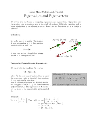
  • 1. Harvey Mudd College Math Tutorial: Eigenvalues and Eigenvectors We review here the basics of computing eigenvalues and eigenvectors. Eigenvalues and eigenvectors play a prominent role in the study of ordinary differential equations and in many applications in the physical sciences. Expect to see them come up in a variety of contexts! Definitions Let A be an n × n matrix. The number λ is an eigenvalue of A if there exists a non-zero vector v such that Av = λv. In this case, vector v is called an eigen- vector of A corresponding to λ. Computing Eigenvalues and Eigenvectors We can rewrite the condition Av = λv as (A − λI)v = 0. Otherwise, if A − λI has an inverse, where I is the n×n identity matrix. Now, in order for a non-zero vector v to satisfy this equation, (A − λI)−1 (A − λI)v = (A − λI)−1 0 A − λI must not be invertible. v = 0. That is, the determinant of A − λI must equal 0. We call p(λ) = det(A − λI) the characteristic But we are looking for a non-zero vector v. polynomial of A. The eigenvalues of A are sim- ply the roots of the characteristic polynomial of A. Example 2 −4 2−λ −4 Let A = . Then p(λ) = det −1 −1 −1 −1 − λ = (2 − λ)(−1 − λ) − (−4)(−1) = λ2 − λ − 6 = (λ − 3)(λ + 2).
  • 2. Thus, λ1 = 3 and λ2 = −2 are the eigenvalues of A.   v1   v2   To find eigenvectors v =  . .  corresponding to an eigenvalue λ, we simply solve the system .     vn of linear equations given by (A − λI)v = 0. Example 2 −4 The matrix A = of the previous example has eigenvalues λ1 = 3 and λ2 = −2. −1 −1 Let’s find the eigenvectors corresponding to λ1 = 3. Let v = v1 . Then (A − 3I)v = 0 gives v2 us 2−3 −4 v1 0 = , −1 −1 − 3 v2 0 from which we obtain the duplicate equations −v1 − 4v2 = 0 −v1 − 4v2 = 0. If we let v2 = t, then v1 = −4t. All eigenvectors corresponding to λ1 = 3 are multiples of −4 1 and thus the eigenspace corresponding to λ1 = 3 is given by the span of −4 . That is, 1 −4 1 is a basis of the eigenspace corresponding to λ1 = 3. Repeating this process with λ2 = −2, we find that 4v1 − 4V2 = 0 −v1 + v2 = 0 1 If we let v2 = t then v1 = t as well. Thus, an eigenvector corresponding to λ2 = −2 is 1 1 1 and the eigenspace corresponding to λ2 = −2 is given by the span of 1 . 1 is a basis for the eigenspace corresponding to λ2 = −2. In the following example, we see a two-dimensional eigenspace. Example     5 8 16 5−λ 8 16 Let A =  4 1 8 . Then p(λ) = det  4 1−λ 8  = (λ − 1)(λ + 3)2     −4 −4 −11 −4 −4 −11 − λ aftersome algebra! Thus, λ1 = 1 and λ2 = −3 are the eigenvalues of A. Eigenvectors  v1 v =  v2  corresponding to λ1 = 1 must satisfy   v3
  • 3. 4v1 + 8v2 + 16v3 = 0 4v1 + 8v3 = 0 −4v1 − 4v2 − 12v3 = 0. Letting v3 = t, we find from the second equation that v1 = −2t, and then v2 = −t. All   −2 eigenvectors corresponding to λ1 = 1 are multiples of  −1 , and so the eigenspace corre-   1     −2  −2    sponding to λ1 = 1 is given by the span of  −1 .  −1  is a basis for the eigenspace       1  1  corresponding to λ1 = 1. Eigenvectors corresponding to λ2 = −3 must satisfy 8v1 + 8v2 + 16v3 = 0 4v1 + 4v2 + 8v3 = 0 −4v1 − 4v2 − 8v3 = 0. The equations here are just multiples of each other! If we let v3 = t and v2 = s, then v1 = −s − 2t. Eigenvectors corresponding to λ2 = −3 have the form     −1 −2   1  s +  0  t.    0 1   −1 Thus, the eigenspace corresponding to λ2 = −3 is two-dimensional and is spanned by  1    0       −2  −1  −2  and  0 .  1  ,  0  is a basis for the eigenspace corresponding to λ2 = −3.         1  0 1  Notes • Eigenvalues and eigenvectors can be complex-valued as well as real-valued. • The dimension of the eigenspace corresponding to an eigenvalue is less than or equal to the multiplicity of that eigenvalue. • The techniques used here are practical for 2 × 2 and 3 × 3 matrices. Eigenvalues and eigenvectors of larger matrices are often found using other techniques, such as iterative methods.
  • 4. Key Concepts Let A be an n×n matrix. The eigenvalues of A are the roots of the characteristic polynomial p(λ) = det(A − λI).   v1   v2   For each eigenvalue λ, we find eigenvectors v =  . .  by solving the linear system .     vn (A − λI)v = 0. The set of all vectors v satisfying Av = λv is called the eigenspace of A corresponding to λ. [I’m ready to take the quiz.] [I need to review more.] [Take me back to the Tutorial Page]