

Recomendados
Más contenido relacionado
La actualidad más candente
La actualidad más candente (20)
Similar a Hypothesis testing
Similar a Hypothesis testing (20)
Hypothesis testing
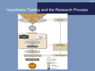
- 1. 18-1 Hypothesis Testing and the Research Process
- 2. 18-2 Types of Hypotheses • Null – H0: µ = 50 mpg – H0: µ < 50 mpg – H0: µ > 50 mpg • Alternate – HA: µ = 50 mpg – HA: µ > 50 mpg – HA: µ < 50 mpg
- 3. 18-3 Two-Tailed Test of Significance
- 4. 18-4 One-Tailed Test of Significance
- 5. 18-5 Decision Rule Take no corrective action if the analysis shows that one cannot reject the null hypothesis.
- 7. 18-7 Factors Affecting Probability of Committing a β Error True value of parameter True value of parameter Alpha level selected Alpha level selected One or two-tailed test used One or two-tailed test used Sample standard deviation Sample standard deviation Sample size Sample size
- 8. 18-8 Statistical Testing Procedures State null State null hypothesis hypothesis s a ho s C tta sho os ttiistt c os e Interpret the Interpret the C iica l e test test al Stages Stages ttes t es t Obtain critical Obtain critical Select level of Select level of test value test value significance significance Compute Compute difference difference value value
- 9. 18-9 Tests of Significance Parametric Nonparametric
- 10. 18-10 Assumptions for Using Parametric Tests Independent observations Independent observations Normal distribution Normal distribution Equal variances Equal variances Interval or ratio scales Interval or ratio scales
- 11. 18-11
- 12. 18-12
- 13. 18-13 Advantages of Nonparametric Tests Easy to understand and use Easy to understand and use Usable with nominal data Usable with nominal data Appropriate for ordinal data Appropriate for ordinal data Appropriate for non-normal Appropriate for non-normal population distributions population distributions
- 14. 18-14 How To Select A Test How many samples are involved? If two or more samples are involved, are the individual cases independent or related? Is the measurement scale nominal, ordinal, interval, or ratio?
- 15. 18-15 Recommended Statistical Techniques Two-Sample Tests k-Sample Tests ____________________________________________ ____________________________________________ Measurement Independent Independent Scale One-Sample Case Related Samples Samples Related Samples Samples Nominal • Binomial • McNemar • Fisher exact test • Cochran Q • x2 for k samples • x2 one-sample test • x2 two-samples test Ordinal • Kolmogorov-Smirnov • Sign test • Median test • Friedman two- • Median one-sample test way ANOVA extension • Runs test •Wilcoxon •Mann-Whitney U •Kruskal-Wallis matched-pairs •Kolmogorov- one-way ANOVA test Smirnov •Wald-Wolfowitz Interval and • t-test • t-test for paired • t-test • Repeated- • One-way Ratio samples measures ANOVA • Z test • Z test ANOVA • n-way ANOVA
- 16. 18-16 Questions Answered by One-Sample Tests • Is there a difference between observed frequencies and the frequencies we would expect? • Is there a difference between observed and expected proportions? • Is there a significant difference between some measures of central tendency and the population parameter?
- 17. 18-17 Parametric Tests Z-test t-test
- 18. 18-18 One-Sample t-Test Example Null Ho: = 50 mpg Statistical test t-test Significance level .05, n=100 Calculated value 1.786 Critical test value 1.66 (from Appendix C, Exhibit C-2)
- 19. 18-19 One Sample Chi-Square Test Example Expected Intend to Number Percent Frequencies Living Arrangement Join Interviewed (no. interviewed/200) (percent x 60) Dorm/fraternity 16 90 45 27 Apartment/rooming 13 40 20 12 house, nearby Apartment/rooming 16 40 20 12 house, distant Live at home 15 30 15 9 _____ _____ _____ _____ Total 60 200 100 60
- 20. 18-20 One-Sample Chi-Square Example Null Ho: 0 = E Statistical test One-sample chi-square Significance level .05 Calculated value 9.89 Critical test value 7.82 (from Appendix C, Exhibit C-3)
- 22. 18-22 Two-Sample t-Test Example A Group B Group Average hourly sales X1 = $1,500 X2 = $1,300 Standard deviation s1 = 225 s2 = 251
- 23. 18-23 Two-Sample t-Test Example Null Ho: A sales = B sales Statistical test t-test Significance level .05 (one-tailed) Calculated value 1.97, d.f. = 20 Critical test value 1.725 (from Appendix C, Exhibit C-2)
- 24. 18-24 Two-Sample Nonparametric Tests: Chi-Square On-the-Job-Accident Cell Designation Count Expected Values Yes No Row Total Smoker 1,1 1,2 Heavy Smoker 12, 4 16 8.24 7.75 2,1 2,2 Moderate 9 6 15 7.73 7.27 3,1 3,2 Nonsmoker 13 22 35 18.03 16.97 Column Total 34 32 66
- 25. 18-25 Two-Sample Chi-Square Example Null There is no difference in distribution channel for age categories. Statistical test Chi-square Significance level .05 Calculated value 6.86, d.f. = 2 Critical test value 5.99 (from Appendix C, Exhibit C-3)
- 26. 18-26 Two-Related-Samples Tests Parametric Nonparametric
- 27. 18-27 Sales Data for Paired- Samples t-Test Sales Sales Company Year 2 Year 1 Difference D D2 GM 126932 123505 3427 11744329 GE 54574 49662 4912 24127744 Exxon 86656 78944 7712 59474944 IBM 62710 59512 3192 10227204 Ford 96146 92300 3846 14971716 AT&T 36112 35173 939 881721 Mobil 50220 48111 2109 4447881 DuPont 35099 32427 2632 6927424 Sears 53794 49975 3819 14584761 Amoco 23966 20779 3187 10156969 Total ΣD = 35781 . ΣD = 157364693 .
- 28. 18-28 Paired-Samples t-Test Example Null Year 1 sales = Year 2 sales Statistical test Paired sample t-test Significance level .01 Calculated value 6.28, d.f. = 9 Critical test value 3.25 (from Appendix C, Exhibit C-2)
- 29. 18-29 k-Independent-Samples Tests: ANOVA • Tests the null hypothesis that the means of three or more populations are equal • One-way: Uses a single-factor, fixed- effects model to compare the effects of a treatment or factor on a continuous dependent variable
- 30. 18-30 ANOVA Example __________________________________________Model Summary_________________________________________ Source d.f. Sum of Squares Mean Square F Value p Value Model (airline) 2 11644.033 5822.017 28.304 0.0001 Residual (error) 57 11724.550 205.694 Total 59 23368.583 _______________________Means Table________________________ Count Mean Std. Dev. Std. Error Delta 20 38.950 14.006 3.132 Lufthansa 20 58.900 15.089 3.374 KLM 20 72.900 13.902 3.108 All data are hypothetical
- 31. 18-31 ANOVA Example Continued Null µA1 = µA2 = µA3 Statistical test ANOVA and F ratio Significance level .05 Calculated value 28.304, d.f. = 2, 57 Critical test value 3.16 (from Appendix C, Exhibit C-9)
- 32. 18-32 k-Related-Samples Tests More than two levels in grouping factor Observations are matched Data are interval or ratio
Notas del editor
- Exhibit 18-1 illustrates the relationships among design strategy, data collection activities, preliminary analysis, and hypothesis testing. The purpose of hypothesis testing is to determine the accuracy of hypotheses due to the fact that a sample of data was collected, not a census.
- The null hypothesis is used for testing. It is a statement that no difference exists between the parameter and the statistic being compared to it. The parameter is a measure taken by a census of the population or a prior measurement of a sample of the population. Analysts usually test to determine whether there has been no change in the population of interest or whether a real difference exists. In the hybrid-vehicle example, the null hypothesis states that the population parameter of 50 mpg has not changed. An alternative hypothesis holds that there has been no change in average mpg. The alternative is the logical opposite of the null hypothesis. This is a two-tailed test. A two-tailed test is a nondirectional test to reject the hypothesis that the sample statistic is either greater than or less than the population parameter. A one-tailed test is a directional test of a null hypothesis that assumes the sample parameter is not the same as the population statistic, but that the difference can be in only one direction. The other hypotheses shown are directional.
- This is an illustration of a two-tailed test. It is a non-directional test.
- This is an illustration of a one-tailed, or directional, test.
- Note the language “cannot reject” rather than “accept” the null hypothesis. It is argued that a null hypothesis can never be proved and therefore cannot be accepted.
- In our system of justice, the innocence of an indicted person is presumed until proof of guilt beyond a reasonable doubt can be established. In hypothesis testing, this is the null hypothesis; there should be difference between the presumption of innocence and the outcome unless contrary evidence is furnished. Once evidence establishes beyond a reasonable doubt that innocence can no longer be maintained, a just conviction is required. This is equivalent to rejecting the null hypothesis and accepting the alternative hypothesis. Incorrect decisions or errors are the other two possible outcomes. We can justly convict an innocent person or we can acquit a guilty person. Exhibit 18-3 compares the statistical situation to the legal system. One of two conditions exists – either the null hypothesis is true or the alternate is true. When a Type I error is committed, a true null is rejected; the innocent is unjustly convicted. The alpha value is called the level of significance and is the probability of rejecting the true null. With a Type II error ( ), one fails to reject a false null hypothesis; the result is an unjust acquittal, with the guilty person going free. The beta value I the probability of failing to reject a false null hypothesis. Like our justice system, hypothesis testing places a greater emphasis on Type I errors.
- Type II error is difficult to detect and the probability of committing a Type II error depends on the five factors listed in the slide. An illustration is provided on the next slide.
- Testing for statistical significance follows a relatively well-defined pattern. State the null hypothesis. While the researcher is usually interesting in testing a hypothesis of change or differences, the null hypothesis is always used for statistical testing purposes. Choose the statistical test. To test a hypothesis, one must choose an appropriate statistical test. There are many tests from which to choose. Test selection is covered more later in this chapter. Select the desired level of significance. The choice of the level of significance should be made before data collection. The most common level is .05. Other levels used include .01, .10, .025, and .001. The exact level is largely determined by how much risk one is willing to accept and the effect this choice has on Type II risk. The larger the Type I risk, the lower the Type II risk. Compute the calculated difference value. After data collection, use the formula for the appropriate statistical test to obtain the calculated value. This can be done by hand or with a software program. Obtain the critical test value. Look up the critical value in the appropriate table for that distribution. Interpret the test. For most tests, if the calculated value is larger than the critical value, reject the null hypothesis. If the critical value is larger, fail to reject the null.
- Parametric tests are significance tests for data from interval or ratio scales. They are more powerful than nonparametric tests. Nonparametric tests are used to test hypotheses with nominal and ordinal data. Parametric tests should be used if their assumptions are met.
- The assumptions for parametric tests include the following: The observations must be independent – that is, the selection of any one case should not affect the chances for any other case to be included in the sample. The observations should be drawn from normally distributed populations. These populations should have equal variances. The measurement scales should be at least interval so that arithmetic operations can be used with them.
- The normality of the distribution may be checked in several ways. One such tool is the normal probability plot. This plot compares the observed values with those expected from a normal distribution. If the data display the characteristics of normality, the points will fall within a narrow band along a straight line. An example is shown in the slide.
- An alternative way to look at this is to plot the deviations from the straight line. Here we would expect the points to cluster without pattern around a straight line passing horizontally through 0.
- This slide lists the advantages of nonparametric tests.
- See Exhibit 18-7, on the next slide, to see the recommended tests.
- The Z test or t-test is used to determine the statistical significance between a sample distribution mean and a parameter. The Z distribution and t distribution differ. The t has more tail area than that found in the normal distribution. This is a compensation for the lack of information about the population standard deviation. Although the sample standard deviation is used as a proxy figure, the imprecision makes it necessary to go farther away from 0 to include the percentage of values in the t distribution necessarily found in the standard normal. When sample sizes approach 120, the sample standard deviation becomes a very good estimation of the population standard deviation; beyond 120, the t and Z distributions are virtually identical.
- The slide shows the six steps recommended for conducting the significance test. The formula for the calculated value is shown here. The t-test was chosen because the data are ratio measurements. The population is assumed to have a normal distribution and the sample was randomly selected. The critical test value is obtained by entering the table of critical values of t (Appendix Exhibit C-2) with 99 degrees of freedom and a level of significance value of .05. We secure a critical value of about 1.65 (interpolated between d.f. = 60 and d.f. = 120 in Exhibit C-2). In this case, the calculated value is greater than the critical value so we reject the null hypothesis and conclude that the average mpg has increased.
- In a one-sample situation, a variety of nonparametric tests may be used, depending on the measurement scale and other conditions. If the measurement scale is nominal, it is possible to use either the binomial test or the chi-square test. The binomial test is appropriate when the population is viewed as only two classes such as male and female. It is also useful when the sample size is so small that the chi-square test cannot be used. The table illustrates the results of a survey of student interest in Metro University Dining Club. 200 students were interviewed about their interest in joining the club. The results are classified by living arrangement. Is there a significant difference among these students? The next slide illustrates a chi-square test.
- The null hypothesis states that the proportion in the population who intend to join the club is independent of living arrangement. The alternate hypothesis states that the proportion in the population who intend to join the club is dependent on living arrangement. The chi-square test is used because the responses are classified into nominal categories. Calculate the expected distribution by determining what proportion of the 200 students interviewed were in each group. Then apply these proportions to the number who intend to join the club. Then calculate the following: Enter the table of critical values of X2 (Exhibit C-3) with 3 d.f., and secure a value of 7.82 at an alpha of .05. The calculated value is greater than the critical value so the null is rejected and we conclude that intending to join is dependent on living arrangement.
- The Z and t-tests are frequently used parametric tests for independent samples, although the F test can also be used. The Z test is used with large sample sizes (exceeding 30 for both independent samples) or with smaller samples when the data are normally distributed and population variances are known. The formula is shown in the slide. With small sample sizes, normally distributed populations, and the assumption of equal population variances, the t-test is appropriate. The formula is shown in the slide. An example is covered on the next slide.
- Consider a problem facing a manager at KDL, a media firm that is evaluating account executive trainees. The manager wishes to test the effectiveness of two methods for training new account executives. The company selects 22 trainees who are randomly divided into two experimental groups. One receives type A and the other type B training. The trainees are then assigned and managed without regard to the training they have received. At the year’s end, the manager reviews the performances of these groups and finds the results presented in the table shown in the slide. To test whether one training method is better than the other, we will follow the standard testing procedure shown in the next slide.
- The null hypothesis states that there is no difference is sales for group A compared group B. The alternate hypothesis states that group A produced more sales than group B. The t-test is chosen because the data are at least interval and the samples are independent. The calculated value is computed as follows: Enter Appendix Exhibit C-2 with d.f. = 20, one-tailed test, alpha = .05. The critical value is 1.725. The calculated value is greater than the critical value so the null is rejected and we conclude that training method A is superior.
- The chi-square test is appropriate for situations in which a test for differences between samples is required. It is especially valuable for nominal data but can be used with ordinal measurements. Preparing to solve this problem with the chi-square formula is similar to that presented earlier. In the example in the slide, MindWriter is considering implementing a smoke-free workplace policy. It has reason to believe that smoking may affect worker accidents. Since the company has complete records on on-the-job accidents, a sample of workers is drawn from those who were involved in accidents during the last year. A similar sample is drawn from among workers who had no reported accidents in the last year. Members of both groups are interviewed to determine if each smokes on the job and whether each smoker classifies himself or herself as a heavy or moderate smoker. The expected values are calculated and shown in the slide. The testing procedure is shown on the next slide.
- The null hypothesis states that there is no difference in distribution channel for age categories of purchasers. The alternate hypothesis states that there is a difference in distribution channel for age categories of purchasers. The chi-square is chosen because the data are ordinal. The calculated value is computed as follows: Use the formula from page 512 The expected distribution is provided by the marginal totals of the table. The numbers of expected observations in each cell are calculated by multiplying the two marginal totals common to a particular cell and dividing this product by n. For example, in cell 1,1, 34 * 16/ 66 = 8.24 Enter Appendix Exhibit C-3 with d.f. = 2, and find the critical value of 5.99. The calculated value is greater than the critical value so the null is rejected.
- The two-related samples tests concern those situations in which persons, objects, or events are closely matched or the phenomena are measured twice. For instance, one might compare the consumption of husbands and wives. Both parametric and nonparametric tests are applicable under these conditions. Parametric The t-test for independent samples is inappropriate here because of its assumption that observations are independent. The problem is solved by a formula where the difference is found between each matched pair of observations, thereby reducing the two samples to the equivalent of a one-sample case. In other words, there are now several differences, each independent of the other, for which one can compute various statistics. Nonparametric Tests The McNemar test may be used with either nominal or ordinal data and is especially useful with before-after measurement of the same subjects.
- Exhibit 18-9 shows two years of Forbes sales data (in millions of dollars) from 10 companies. The next slide illustrates the hypothesis test.
- The null hypothesis states that there is no difference in sales data between years one and two. The alternate hypothesis states that there is a difference. The matched or paired-sample t-test is chosen because there are repeated measures on each company, the data are not independent, and the measurement is ratio. The calculated value is computed as follows: Use the formula from page 514 Enter Appendix Exhibit C-2 with d.f. = 9, two-tailed test, alpha = .01, and find the critical value of 3.25. The calculated value is greater than the critical value so the null is rejected. We conclude that there is a significant difference between the two years of sales.
- In a fixed-effects model, the levels of the factor are established in advance and the results are not generalizable to other levels of treatment. To use ANOVA, certain conditions must be met. The samples must be randomly selected from normal populations and the populations should have equal variances. The distance from one value to its group’s mean should be independent of the distances of other values to that mean. Unlike the t-test, which uses sample standard deviations, ANOVA uses squared deviations of the variance to that computation of distances of the individual data points from their own mean or from the grand mean can be summed (recall that standard deviations sum zero). In an ANOVA model, each group has its own mean and values that deviate from that mean. The total deviation is the sum of the squared differences between each data point and the overall grand mean. The total deviation of any particular data point may be partitioned into between-groups variance and within-groups variance. The between-groups variance represents the effect of the treatment or factor. The differences of between-groups means imply that each group was treated differently and the treatment will appear as deviations of the sample means from the grand mean. The within-groups variance describes the deviations of the data points within each group from the sample mean. It is often called error.
- The test statistic for ANOVA is the F ratio. Use formula from page 517 To compute the F ratio, the sum of the squared deviations for the numerator and denominator are divided by their respective degrees of freedom. By dividing, we are computing the variance as an average or mean, thus the term mean square. The degrees of freedom for the numerator, the mean square between groups, are one less than the number of group (k-1). The degrees of freedom for the denominator, the mean square within groups, are the total number of observations minus the number of groups (n-k). If the null is true, there should be no difference between the population means and the ratio should be close to 1. If the population means are not equal, the F should be greater than 1. The F distribution determines the size of the ratio necessary to reject the null for a particular sample size and level of significance.
- To illustrate, consider the report about the quality of in-flight service on various carriers from the US to Europe. Three airlines are compared. The data are shown in Exhibit 18-11. The dependent variable is service rating and the factor is airline. he null hypothesis states that there is no difference in the service rating score between airlines. ANOVA and the F test is chosen because we have k independent samples, can accept the assumptions of analysis of variance, and have interval data for the dependent variable. The significance level is .05. The calculated F value is 28.30 (see summary table in the last slide). Enter Appendix Exhibit C-9 with d.f. = 2, 57, and find the critical value of 3.16. The calculated value is greater than the critical value so the null is rejected. We conclude that there is a significant difference in flight service ratings. Note that the p value provided in the summary table can also be used to reject the null.
- In test marketing experiments or ex post facto designs with k samples, it is often necessary to measure subjects several times. These repeated measures are called trials. The repeated-measures ANOVA is a special type of n-way analysis of variance. In this design, the repeated measures of each subject are related just as they are in the related t-test where only two measures are present. In this sense, each subject serves as its own control requiring a within-subjects variance effect to be assessed differently than the between-groups variance in a factor like airline or seat selection. This model is presented in Exhibit 18-17.