1. Experiment 3
Filters II – Filter Design with MATLAB
The objective of this experiment is to gain some experience in designing filters with
desired specifications. You will work with a number of tools helping you in designing filters
in MATLAB.
Prelab
P1. Review of Filters – Frequency Domain
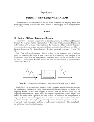
The effect of a system on a signal input to it can be described in both time and frequency
domains. We observed the time representation of the system in last experiment. Here we will
study the frequency domain representation of the system as a filter. Different frequency
components of the input signal experience different attenuation/amplification and delays as
they pass through the filter thus a filter alters the signal input to it in frequency domain (Fig.
P1).
One of the main applications of a filter is to filter out the unwanted parts of an input
signal. The unwanted part might be noise present out of the frequency band occupied by the
desired signal (high frequency noise) or other interfering signals that are unwanted, e.g. when
you tune to a radio station, the radio receiver will filter out other stations so you would hear
a clear sound (Fig. P2).
f f
Figure P1 – The alteration of frequency components of a signal input to a filter
Simple filters can be categorized into four major categories: lowpass, highpass, bandpass
and bandstop (or band-reject). Figure P3 shows the ideal forms of these four filters in the
frequency domain. As the name suggests a lowpass filter for instance, passes the low
frequency components of a signal while blocking the high frequency ones. As you have
learned the convolution operation in time domain is equivalent to multiplication in
frequency domain. Thus, multiplying the frequency domain representation of the input
signal with that of the filter, high frequency components of the input signal will be multiplied
in zero and would thus vanish, while the lower frequency components will be multiplied by
one and would pass without any change.
1

2. Noise
f f
Interfering stations
Desired station f f
Figure P2 – Some basic applications of filters: top) noise reduction by removing out of band
(high frequency noise), bottom) removing interfering signals: passing of a tuned channel in a
radio.
In this experiment you will learn how to use some tools in MATLAB signal processing
toolbox to design filters with your desired characteristics.
f f
f f
Figure P3 – The ideal frequency response of the four basic filter types: 1) lowpass,
2) highpass, 3) bandpass and 4) bandstop (or band-reject)
2

3. P2. Filter Design
Before designing a filter, you should know what parameters need to be known for the
design.
The ideal filters as shown in figure P3, cannot be physically realized, since they are non-
causal, i.e. to generate the output at instance n in time, they require the knowledge of future
samples of the input signal, i.e. at n + 1, n + 2,... , which is impossible. The design techniques
are as a result, approximations of the ideal case.
The digital filter design methods fall into two main categories, FIR filter design and IIR
filter design. You will learn more about these types in your future courses. In this experiment
you will be introduced to some tools for basic IIR filter design.
First of all you should know the parameters of the filter that you are going to design.
Some of these parameters are described in this section.
dB Notation
Something you will very often encounter when dealing with filters is the deci-Bell (dB)
notation. The reason is that when you’re dealing with a wide range of variation in the
magnitude of a quantity, say 5 orders of magnitude difference between maximum and
minimum, it is hard to work with the numbers. If you use the logarithm of the magnitude,
the variations will be too small! So Alexander Graham Bell, invented this new notation
named after him by using 20 times the logarithm of the magnitude. Thus
x dB = 20 log 10 x ⇔ x = 10 x dB 20
Some figures that you should know without using your calculator are 3 dB and its
multiples. 3 dB is almost equal to 2, thus if you have a quantity that is 3 dB greater than
another, it is actually two times greater than it. (Note that you are using logarithm, thus
addition of the logarithms is equivalent to multiplication of the numbers themselves.) By
analogy, -3 dB, 6 dB and -6 dB are equivalent to 0.5, 4 and 0.25 respectively.
Passband Parameters
The passband of the ideal filter is the band of frequencies where the filter frequency
response is not zero. If a signal’s frequency content lies in this band, the signal will pass
without any alteration. In case of practical filters, the frequency response does not have an
abrupt change from zero to one or the value in passband (Fig P4). Instead, there is a
transition from a higher level to a lower level. Hence, for a practical filter the band of
frequencies over which the magnitude of frequency response is greater than a threshold is
called the passband. This threshold is usually set at -3 dB of the maximum magnitude in
passband. The frequency at which the filter’s frequency response magnitude reaches this
threshold is called the cut-off frequency of the filter ( f c ) .
If the frequency response does not decrease monotonically in the passband the filter is
said to have ripples in the passband. The difference between the maximum and minimum
magnitude values in the passband defines the passband ripple factor R p usually given in
dB. The maximum value of the magnitude in passband is called the gain of the filter.
Stopband Parameters
The stopband of the ideal filter is the band of frequencies where the filter frequency
response is zero. Thus the frequency components of the signal lying in this band will not
3

4. pass and will be fully removed. Again, since the transition from high to low is not abrupt in
practical filters, a threshold level defines this region. So, the band of frequencies, where the
magnitude of the frequency response of the filter drops below a threshold level is called
stopband. The threshold value is dependent on the application of the filter usually about 40
dB and is usually denoted by As or Rs .
If there are ripples in the stopband, the maximum value of the magnitude of frequency
response in the stopband shall lie below the threshold. The frequency at which the
magnitude of the filter response first falls below the threshold value is called the stopband
frequency denoted by f s .
Figure P4 – The filter parameters: 1) passband, 2) stopbands, 3) cut-off frequencies,
4) stopband frequencies, 5) passband ripple, 6) stopband level, 7) filter gain.
P3. Four Classical IIR Filter Types
In this section I will introduce and compare the four classical IIR filter types, namely
Butterworth, Chebychev Type I and II, and Elliptic filters. You will encounter these
filters and probably their design methodologies in your future courses. Since
straightforward algorithms for design and implementation of these filters exist, many
software programs help you in designing these filters by simply specifying their
parameters. Hence, for the sake of this experiment you need not know all the
mathematical detail involved in the design of these filters1. All filters here refer to the
lowpass case. You can simply generalize the results to the other types by analogy.
1
If you are interested in further study of these details you may refer to “Digital Signal Processing, System
Analysis and Design”, by P.S.R Diniz, E.A.B. da Silva and S.L. Netto, Cambridge University Press, 2002
4

5. Butterworth Filter
The Butterworth filter of order N , also called the maximally flat filter, is an
approximation of the ideal filter, which the first 2 N − 1 derivatives of its magnitude squared
are zero. As a result the frequency response of this filter decreases monotonically with
frequency and H ( f = f c ) = 1 2 . The decrease is very slow in the passband and quick in
the stopband. In a design problem where no ripple is acceptable in passband and stopband,
Butterworth filter is a good choice.
Figure P5 – The frequency response of a Butterworth filter with ωc = 1
Chebychev Type I Filter
A Chebychev type I approximates the ideal filter by minimizing the absolute difference
between the resulting filter and the ideal filter, over the passband. This filter results in
appearance of ripples in the passband. The ripples have a constant magnitude of R p which is
one of the design parameters of this filter. The stopband response is maximally flat. The
transition from passband to stopband occurs faster than the Butterworth filter:
H ( f = f c ) = R p . If the ripples in the passband are acceptable, a Chebychev filter usually
require a lower-order transfer function than a Butterworth filter for the same specifications.
Figure P6 – The frequency response of a Chebychev type I filter with ωc = 1
5

6. Chebychev Type II Filter
A Chebychev type I approximates the ideal filter by minimizing the absolute difference
between the resulting filter and the ideal filter, over the stopband. This filter results in
appearance of ripples in the stopband. The ripples have a constant magnitude of Rs which is
one of the design parameters of this filter. The passband response is maximally flat and
H ( f = f c ) = Rs . The transition from passband to stopband occurs slower than the type I
filter and for even filter order, it never reaches zero. Its advantage over type I is the absence
of ripples in the passband.
Figure P7 – The frequency response of a Chebychev type II filter with ωs = 1
Elliptic Filter
The elliptic filter results in the steepest transition from passband to stopband by allowing
ripples in both passband and stopband. This filter usually satisfies the desired filter
specifications with the lowest order among the four types studied. The passband and
stopband ripples R p and Rs are also required as design parameters.
Figure P8 – The frequency response of an elliptic filter with ωc = 1
6

7. MATLAB sptool: Filter Design and Signal Processing Tool
1. Adding Phone Effect to a Sound
In this section you will learn how to use a powerful signal processing tool in MATLAB,
sptool which is part of the MATLAB’s signal processing toolbox and helps you with filter
design and signal processing with an easy to use GUI.
In what follows, you will design a bandpass filter that resembles the bandpass filter in a
telephone system. You will then apply this filter to the French speaker sound file you used
before, to create a phone effect to the sound.
• At MATLAB command prompt type sptool.
• In the Filters list click on the New button. This creates a new filter design.
• In the sampling frequency edit box enter 11025 as the sampling frequency.
• From the algorithm dropbox, select Butterworth IIR filter.
• Select bandpass in the filter type dropbox.
• Enter 200 and 1200 for the low and high stopband frequencies respectively.
• Enter 250 and 1000 for the low and high passband frequencies respectively.
• Click the Apply button at the bottom of the left panel.
• Close the filter design tool.
Your filter is now designed and ready for use! You should import the French speaker’s
sound file into sptool, apply your filter to it:
• At MATLAB command prompt load the .wav file ‘french.wav’.
• Downsample the sound from 44100 to 11025Hz (don’t forget to update FS).
• In sptool, in File menu select Import…
• Set Import as to signal.
• Select from workspace and select the name of the vector containing the sound data and
click the right arrow to import the data
• Select the sampling frequency from the workspace variables and import it.
• Enter a name for the imported signal, the default is sig1.
• Click OK to complete import.
• From the Filters list select your filter design and click the apply button.
• Leave the defaults as they are and click OK.
• In the Signals list, you will see the result of filtering, select it, hold down control key and
select the input signal.
• Click the View button.
• If you can’t see both signals, click on the select trace in the toolbar and select the
output signal.
• Click the play sound in the toolbar to listen to the output.
• Switch the selected trace from output to input, play the signals and note the difference.
Now go back to filter design screen to compare different filter design methods with each
other.
• Make sure the value of R p is set at 3 dB and Rs at 20 dB.
7

8. • Note the shape of the Butterworth filter response and specifically the stopband
frequencies.
• Now change the filter type to Chebychev type I.
• Take note of the actual stopband frequencies and the shape of the filter response.
• Repeat for the Chebychev type II and elliptic filter types. What is your deduction?
To view the impulse response of each filter, go back to sptool main window and select
your filter and click the View button. A new tool window appears. You may see the phase
and amplitude response of the filter you have designed in this window. From the left panel,
check the Impulse Response. Use the zoom tool , to zoom in and see the first portion
of the response. Use the zoom all tool , to select another potion or use the zoom tool to
zoom in again.
Uncheck the Magnitude and Phase boxes and check the Zeros and Poles. Zoom out to
see the full plot. In the design window, change the filter type. What happens to the position
of the poles and zeros? Can you compare the four basic designs?
2. Out of Band Noise Removal
In this part you will use a lowpass filter to remove the high frequency noise in a signal.
• At MATLAB command prompt use size command to determine the number of
samples in the downsampled French speaker sound you loaded before.
• Generate a random noise vector n with the same number of samples as the French
speaker’s signal. Use MATLAB randn command to generate the noise vector whose
samples have Gaussian probability distribution. Scale down the noise by multiplying your
vector by 0.1.
• Add the noise and your original sound to make a new vector. Make sure you don’t
destroy your original sound file.
• Import the noise and the noisy sound in sptool.
• View the noise, noisy sound and the original sound using View button.
• Listen to the three signals.
• Now design a lowpass filter with following specifications:
o f c = 1500 Hz and f s = 1650 Hz.
o No ripple in passband is allowed.
o Your filter order should not be more than 15. (Check the right panel to see the
order of your filter)
o Rs should be at least 30 dB.
• Apply your filter to the noise signal and to the noise.
• View the results and signals before filtering.
• Listen to them and compare them.
Now try to export your filter design to MATLAB:
• In sptool main window in File menu select Export…
• Select your filter name in the left panel
• To see the transfer function of the filter, check the Export Filter as TF Object.
8

9. • Click the Export to worksapce button.
• At MATLAB command prompt, type the name of your filter design to see its transfer
function. You will see the name of your filter in MATLAB’s workspace panel.
• Return to sptool and again export your filter design now with the Export Filter as TF
Object unchecked. Confirm replacement of your old workspace filter export.
• At MATLAB command prompt, type the name of your filter you should see something
like this:
filt2 =
tf: [1x1 struct]
ss: []
zpk: [1x1 struct]
sos: []
imp: []
step: []
t: []
H: [1x4096 double]
G: [4096x1 double]
f: [1x4096 double]
specs: [1x1 struct]
Fs: 11025
type: 'design'
lineinfo: [1x1 struct]
SPTIdentifier: [1x1 struct]
label: 'filt2'
You will see the name of your filter instead of filt2.
• To access the transfer function parameters of your filter use this syntax and replace filt2
with your filter’s name: filt2.tf.num to see the numerator coefficients of your filter
and filt2.tf.den to see its denominator coefficients.
• You may access the other parameters of the filter, like location of poles and zeros and
sampling frequency in the same way.
9