SlideShare una empresa de Scribd logo
1 de 39
Descargar para leer sin conexión
AGE AND GROWTH OF THE ANTARCTIC FISH Chaenocephalus
aceratus based on OTOLITH weight, microstructure and TL frequency;
some relations with Pseudochaenichthys georgianus.
39 pages
Ryszard Traczyk1
ABSTRACT
Chaenocephalus aceratus were sampled in the summer between 1979
and 1990 at South Georgia. The otoliths of C. aceratus contained
microincrements similar to daily increments in the otoliths of fishes from
temperate and tropical waters. The estimated age from microincrements was
similar to that inferred from otoliths weight distribution. Changes of the
microincrements growth pattern are described that appear to be related to
larval, hatching and metamorphosis, and have similar pattern to that ones
described for Ps. georgianus. Both species have similar life history, that
reflect in their close up otoliths morphology. The ages of 29 individuals of C.
1 M.Sc., on permanent disability payment, address: ul. Orkana 47/8, 34-700 Rabka-Zdrój, Poland, phone +48 018
2676783, email: soplik@op.pl.
-1-
Fig. 1: R/V "Professor Siedlecki" in Antarctica on expedition in 1988/89; fish sample on board and ordered by species.
aceratus were determined by microincrements. The age of fish sampled by
the fishery (Fig. 1) was predicted from otolith weight using a regression
equation. In the other way the age of fish was determined from otolith weight
frequency and its modal progress analysis. The results from those methods
were compared to each another through the study of spawning, hatching and
metamorphose marks in otolith, by back calculating procedure, by length
frequency analysis and by comparison with the literature. For C. aceratus the
von Bertalanffy growth parameters were, k = 0.26, L∞ = 75, t0 = 0.51. Otoliths
size at age, with corrected variability for 3 dimension were established, Tab.
3.
INTRODUCTION
Chaenocephalus aceratus like other Channichthyidae is a cold adapted fish
living exclusively in Antarctic waters. They have low metabolism, prolonged
oogenesis, delayed maturation, slow growth, large yolky eggs and iteroparity. Larval
stages hatch at large size and at a relatively advanced stage of development.
Reproductive cycles appear to be closely linked to the production cycle so that young
develop during period elevated production[10]
. Channichthyidae have no red blood
cells or any oxygen binding pigment. In part compensation directed to increase
oxygen respiration are: large head and fins.
C. aceratus is distributed in Bouvier Island, islands of the Scotia arc (South
Georgia, South Sandwich, South Orkney, and South Shetland Islands) and the
Antarctic Peninsula in range of depth from 5 to more 770 m[3]
. In the South Georgia -
most numerous, in South Orkneys and in the South Shetlands less numerous.
There is a succession of species hatching throughout winter to summer at South
Georgia. The order of hatching was familial - a bathydraconid then channichthyids,
followed by the nototheniids. Their feeding periods are likely to be broadly
synchronized with the life cycles of their food species. Their food may be limiting the
amount of larvae which can coexist in the ecosystem at any given time of year.
Clarke (1988)[9]
postulated that production (growth and reproduction) of polar marine
-2-
ectoterms is limited not by the temperature but by the food availability and that the
seasonality of their growth is linked to their position in the food web. Different life-
history stages live at different mean depths and distance from the shore, the diet
varied for them (Burchett at all 1983)[2]
. The adults usually occupying the deepest
waters[9]
about eight times numerous between 150 and 250 m depth than upper or
lower[12]
. Their diet varied during the life cycle, further from the shore adults fed
mainly upon mysids and fish (Permitin and Tarverdiyeva 1972[12]
). Inshore juvenile
feed mostly on decapods shrimps and fish (Burchett at all 1983)[2]
. Postlarval and
juveniles' forms were lived in the pelagic zone often with krill[6 ,5]
Antarctic fish
concentration were located very close to the bottom during the day and dispersed into
the water column after dark by the echo sounder[12]
. The feeding behaviours as well as
habitat varied during their life cycle. Seashore they display a high level of nocturnal
activity linked to as much of the benthos is also more active at night. Offshore
feeding insensitivity of adults is probably highest during the day as was find for N.
rossi by Linkowski and Rembiszewski[6]
with assumption of Burchett and other,
1983)[2]
. In late summer they in schooling move inshore to 240 m depth, from the
shelf areas to spawn (Burchett and other, 1983)[2]
. At South Georgia spawning occur
over limited time period from the end of February to the end of April. With another
data spawning: 1) at South Georgia: from March to May (egg are laid from March to
May); length at first spawning - 58.4 cm TL for females and 47.5 cm TL for males; 2)
at Elephant I., from May to June; length at first spawning - 57.1 cm TL for females
and 45.7 cm TL for males.
Chaenocephalus aceratus has a relatively high growth rate, but becomes
sexually mature at a relatively large proportion of maximum length. By adopting a
strategy of growing rapidly to a large size before reproducing, this species can
predate a wide size range of fish and so increase its tropic scope. C. aceratus matures
at a relatively large size and would therefore be expected to exhibit delayed
maturation but the rapid growth rate of this species compensates and so the age of at
maturity falls within the trend observed for other notothenioids[9]
. Males mostly are
smaller by 101 mm than females. Maximum theoretical length of female is 76.5 and
-3-
male 58 and is related to the size and age at sexual maturity, that are a half to three-
quarters of above data 40 - 50 cm with age of seven for female and six for male[5]
.
The rate of growth to asymptotic size (K) is related to size and age at sexual maturity
(0.17 male; 0.24 female[5]
).
Length distribution of C. aceratus shows modes at 18 (21g) and 26 cm (90 g),
but for longer fish it become indistinct due to differences between the sexes. There is
good agreement between the mean length at age and the modal lengths for first two: 1
– 18 cm and 2 – 26 cm age groups. The other follows as in Tab. 1.
Tab. 1: Mean length and weight at age of male and female C. aceratus, after Parkes[11]
Age: 1 2 3 4 5 6 7 8 9
♂♂[cm] 18 26 32.6 38.2 45.3 49.4 50.4
♂♂[g] 21 90 197 350 641 871 945
♀♀[cm] 47.4 51.9 57 59.7 61.9
♀♀[g] 756 1050 1464 1726 1988
There was a significant difference between mean length and weight at age of
male and female C. aceratus above age 5, Tab. 1. Males of age 7 were on average
nearly 7 cm shorter than females of the same age[11]
. Previous age data: juveniles
from 26 to 35 cm - III and IV age classes.
The spawning and the hatching of the early larvae were probably less dictated
by occurrence of immature copepods - common food of early larvae of fish.
The Antarctic marine environment is highly seasonal with a strong pulse of
production occurring over the summer period and minimum in winter (Clarke,
1988[9]
). The timing of spawning and subsequent hatching of larvae in relation to this
annual cycle will largely determine the amount of food available to them. Copepods
have a life-cycle that is closely linked to the primary production cycle and their
abundance parallels phytoplankton productions with high level for most of the
summer period from November to February at South Georgia[9]
. In advance of the
peak in production cycle C. aceratus as same Antarctic species lay large yolky eggs
which hatch the large larval stages during autumn and winter[9]
. They survive winter
by feeding on the overwintering stages of neritic copepods and thus their life cycles
-4-
are not directly linked to above mentioned high abundance secondary production. In
spring they are able to prey upon larval fish which hatch in this period in addition to
feeding on other zooplankton. Therefore hatching early in the season seems to be
advantageous to species which are piscivorus as larvae (North and Ward 1989[9]
).
C. aceratus eggs are yolky and large between 3.9 - 4.7 mm in diameter, and in
consequence the fecundity is low (5 - 9 egg by fish total weight in gram)[9]
. They have
biennial (two years) process in the development of mature oocytes[10]
. Size of ripe
eggs is: 4.4 - 4.7 mm in diameter. They are laid demersal at depth of 240 m from
March to May. When eggs spawned their development period to hatching is one or
two month[2, 9]
. C. aceratus have extended hatching period: at Antarctic Peninsula is
from August to October; and at S. Georgia, It hatch early - in winter (June -
November) have 11 - 17 mm total length (as size of eggs) with large yolk sac (about
50 % of the body mass), that is probably utilized within two months of hatching[9]
.
Larvae are of apterolarval form, and not especially advanced in overall development,
although they are somewhat precious because they can soon feed. They have a better
muscle arrangement for cruise swimming than the adults, in which slow muscles are
only a minor component of the trunk muscles[9]
.
As the yolk-sac is absorbed, the larvae commence feeding and this is also a
future of Antarctic fish larvae (North and Ward 1989[9]
). Their heads and jaws are
large enough, Fig. 2, 13, to feed on
the overwintering stages of small
copepods, such as Drepanopus
forcipatus[9]
. Hatching spread to
four months period producing
larvae in sequence reduces the potential for interspecific competition within the
ichthioplankton[9]
. First individuals to appear preceded the period of increased
copepod abundance (by up to five month) feed on small copepods grow sufficiently
large to adopt a piscivorus diet when the larval stages from species that breed later
arrive in the plankton[9]
. They can feed on high level abundance of copepods in spring
and summer. The growth rate of larval C. aceratus of 15 - 40 mm SL was about 0.11
-5-
Fig. 2: Chaenocephalus aceratus, larva, 2.1 cm, after North.
- 0.16 mm SL per day at the Antarctic Peninsula[12]
. There are differences in data,
Tab. 2, that could be explained by extended hatch period, as it was stated by
Ślósarczyk[12]
(early in August hatch larva after 6 months in January could be as 8 cm
juvenile).
Tab. 2: Published data length during larval development
August November-early December January-March
cm SL cm SL cm SL
1.5 – 1.8 with yolk sac 1.9 – 4.0 with yolk sac 2.2 – 2.3 with yolk sac
– 8.0 3.3 – 5.9 to February
The larval length span to metamorphosis ranges up to 80 mm (probably in
December? Tab. 2) and is over than a typical tropical fish[9]
. They growth to the
juvenile stage during six, seven month (juvenile were found in January) and it is long
period in compare with weeks or days for temperate and tropical marine fish[9]
.
In late winter larvae within 5 km of the coast of the island were with large
shoals in sublittoral waters (less than 40 m depth)[7]
. Near the coast at South Georgia,
C. aceratus are in most abundant group of larvae in September (early spring) in
compare with other months in which the most abundant are different species[8, 7]
. In
early spring the number of C. aceratus larvae as piscivorus is about one-tenth[9]
.
In summer the larvae at South Georgia undertook diurnal vertical migrations,
when phyto and zooplankton abundance are high[8, 7]
.
The family Chaenichthyidae provide difficult in age estimation. The methods
based on counting annuli marks in otoliths give some mistrust. They show several
mark that difficult interpreted and to relate. Daily increments account can verify
them. They can give information on seasonal increase, decrease or lack of growth of
fish, and morphological and physiological change and shift like change of
environment, metamorphose, maturing, spawning and other. This could calibrate the
fishing predict of icefish C. aceratus that were exploited since 1977. Foremost in the
elucidation of accurate population dynamics' parameters in fish is the correct
-6-
estimation of age. So here will be try to assess alternative methods of determining the
age of the fish from the otolith by comparing ages based on otolith biometry and
morphology (height, mass, otolith shape the last, number of primordia was used by
Prof A. Kompowski – personal communication), with those derived from internal
microincrements. Some additional data on their relations to one to another will be
added.
The main objective of the present work was to study daily increments of C.
aceratus to show biological data and next compare Ps. georgianus and C. aceratus
appearances, life stages, behaviours that determine otolith morphology - Ps.
georgianus and C. aceratus have similar otoliths and daily increments.
MATERIAL, METHODS
The sets of ichthyological data on C. aceratus, Fig. 3, collected during three
Antarctic expeditions in 1979 (by Polish sciences, Fig. 1), 1990 (by English - Polish
FSA sciences group) and in 1986 in the South Georgia area in the summers were
-7-
Fig. 3. Champsocephalus aceratus, 58 cm TL, during collecting data: length, weight, sex, maturity.
taken into account. The otolith was chosen as the best structure for age determination
from the other hard structures of this fish (based on published CCAMLR guidelines).
Fish were measured and weighed and their sagittal otolith were removed and stored.
Age was determined by length frequency analysis.
Age determination from the otolith
Otoliths were cleaned with a commercial solution of Clorox (5.25% sodium
hypochlorite), washed with water, dried, weighted (accuracy ±0.1 mg). Otolith's
microincrements and other features were examined using various methods including,
light microscopy with transmitted and reflected light,
and scanning electron microscopy (SEM).
Age was determined in relation to
measurements of the otolith external and internal
morphometry. To establish the development of the
shape of otolith, changes in microincrements pattern,
and their distances from the centre was measured in
transverse sections (Fig. 4).
Whole dried otoliths of all sizes were
embedded in epoxy resin in bars and
ground on two parallel sides with
carborundum paper (No. 80-800) to
reveal the nucleus and then mounted
in Eukitt (microscopic mounting
medium) directly on microscopic
slides, Fig. 5, 6. These were ground
and polished with a 1 µm diamond
compound by hand and grinding
machine under water to the thickness
of 0.1-0.15 mm to view the
microincrements. Sections were
released from Eukitt with chloroform
-8-
Fig. 4: Otolith C. aceratus
M-S
plane
Tplane
R
0
1
2
3
mm
Fig. 5: Otoliths embedded in resin and mounted on slides.
Numbers were draw by diamond on glass, glasses are not show
in all ranges.
0 1 2 3 4 5 6 7cm
or xylene.
Growth pattern from the polished
sections were measured. This included
recording the width and position of each
microincrement and opaque and hyaline
zones from centre of the otolith to the edge.
Etched sections.
To reveal incremental patterns in the
surface relief of some polished sections they
were etched for 1 - 8 minutes with EDTA.
This was on both sides for C. aceratus
because their microincrements were visible in
light microscope when the both sides of
otolith slides were etched. They were cleaned
with water and dried. The etched surface was pressed into acetone soaked acetate
sheets paper to produce acetate replicas. Dried acetate replicas were photographed.
Etched otoliths were coated with a nano- thickness of gold using an electric arc
current at an angle of 45º in a vacuum (9.4·10-8
Tr). They were examined by reflected
light microscopy. The growth pattern was observed - the positions of ditches created
by removing of calcium and corresponding to micro-opaque zones in polished
sections, were photographed. Etched and coated otoliths were also examined by
scanning (SEM). Microscopic slides, Fig. 5, 6, with one or more coated otolith
sections were attached to custom made SEM stubs (the metal plate of the slides size
were welded to standard stubs with the connecting metal string to the coated surface),
Fig. 7. SEM screen projections of the coated otolith sections were photographed to
produce their
film negative
for further
analysis and
to
-9-
Fig. 6: Preparing otoliths from larvae and
postlarvae, glasses are not show in all ranges
0 1 2 3 4 5 6 7cm
Fig. 7: preparing sample to SEM
coated glass surface with gold
put
connect
metal
metal
microincrements counts by direct measure and count from photograph. The micro-
opaque zones appeared dark maxima on the negatives.
Age differentiation based on otolith morphology.
The parameters of otolith surface morphology were analysed in relation to the
fish and otolith size to examine changes in otolith shape during growth.
Analysis of the otolith size.
The otolith sizes (their limits on the T planes, otolith weight) were analysed by
age. Means, variances and standard deviations of the measurements were compared
and tested for differences.
Back calculations.
Assumed little individual variability in the otolith size age relationship
permitted the prediction of past growth from the otolith size. Past growth was
predicted from the linear regression model of the size of otolith and fish total length
relationship.
Age determination from otolith weight.
The Bhattacharya method[3]
was applied to determine age from otolith weight
frequency. The left skewness: values on left that are less then mean of groups in the
otolith weight frequency were linearised and fitted by the normal distribution whose
digits as first age group were subtracted. From remained data its new left skewness
were analysed as above to get second age group and after that next older ones. To that
age group in otolith ordered weight data (usual 4 groups) their appropriate data fish
length data were then taken by that age group. Obtained length frequency of 3 - 4 age
group in this way were basis to take into account Bertalanffy growth formula (growth
of fish from first to second and next age group) to additional approximate the mean of
age group and then to fit correct distribution of age groups in otolith weight
frequency and length frequency.
Estimate the age of the largest samples.
Otolith morphometry were related to age. The relationship between otolith
weight and age were used to extrapolate the ages of the largest fish. Where, ages in
days were determined by counting microincrement.
-10-
Analysis of otolith weight frequency at age modes for year sample.
The frequency distributions of the measure variables were examined from the
larger 3 year sample to detect modes associated with individual cohorts (year-
classes). Only data for one season of the year was used. The mean and the standard
deviation of otolith parameters of that cohort were examined for variation within and
between cohorts by years. The progression of modes in the otolith weight frequency
during ontogenesis was analysed to separate age groups and derive growth age
groups.
The mean size of each age class derived from polymodal frequency analysis of
otolith weight was statistically compared (using Least Significant Difference test[1]
).
And where they agreed a combined age was produced.
Age determination from length frequency.
Age determination by Bhattacharya method.
The length frequencies were taken from 3 year sample. The left skewness in
the length frequency (values on left that are less then mean of group in the TL
frequency) were linearised and fitted with the normal distribution. Then the digits as
first age groups were subtracted. From remained data its new left skewness were
analysed as above to get second age group and after that next older ones. To that age
group in fish length the Bertalanffy growth formula was fitted, from which the mean
of further age group were predicted. Based on obtained averages of older fish and
remained modal frequencies at age (after subtraction frequency of younger age
group) the frequency of older fish were estimated and corrected formulas of
Bertalanffy equation were then established (on means of age groups).
Analysis the progression of age modes during ontogenesis.
Sequences of length composition at annually progressing one age group were
analysed throughout ontogenesis to get information on the annual growth rate of
population of one this same age. Difference among the years were subject to estimate
and predict the annually changes in averages of length and in numerous of fish to the
stock predict.
Fish growth parameters
-11-
The Bertalanffy growth model[4]
was fitted to each set of age data from each
method of age determination.
Age data was transformed to catch frequency by the Gulland[4]
equation: (NiPij)
to age at length of the catch frequency, where Ni is the number of fish in i-th. Length
class from catch length measure in the season, the Pij is the following proportion: Pij =
nij/ni (ni - the number of fish in i-th. length class; nij - the number of fish in i-th. length
class and in j-th. age groups). Then they were used to calculate theoretical growth of
fish using the von Bertalanff'y equation. Age data were arranged as available cached
set of age groups within one season, that were simplify to within one age population
during it ontogenesis.
RESULTS
The growth zones of otolith
Daily zones
With sectioning and polishing there were micro increments visible. Otolith
sections of 29 individuals viewed by the light microscopy showed incremental
patterns that were measured and counted (Fig. 9). The manner of increments was
observed also on acetate replicas and with SEM, Fig. 8.
In the central area of otolith, daily increments were wider, and mostly had 2.5-
4 μm – at distance ~0.002 mm from the centre, Fig. 10, 11. At distance ~0.06 mm
daily increments were relatively similar: 2-3.3 µm. But at outer layers up to 0.7 mm
distance from the center, increments were very narrow: 1.1-2 µm. At larger distance
from the center, the widths of daily increments were alternately wide follow after the
small and after them wide again. Apart from that wide – small – wide alternate
pattern the increments' width decreasing from the center to the otolith edge in
general: at 0.83 mm from the center increments were 2-2.5 µm wide; at 1.43 mm
from the center there were 1.29 µm wide; at 2.15 mm there were 1.1-1.25 µm. In
average for specified distance from the center there were 3 up to 9 daily increments
per 10 µm. That unit was useful for correcting data for adequate sectors with partially
destroyed surfaces.
-12-
-13-
Fig. 8: SEM microphotograph of otolith daily increments of C. aceratus.
-14-
Fig. 9: Microincrements from the transverse section of a sagittal otolith from 45 cm TL C. aceratus applied to daily
increment count. From central primordium, CP to the otolith edge there are 1590 days.
C
B
1590 incr., 2.347 mm
554 incr., 0.816 mm
48 incr., 0.046 mm
+1036 incr.
+506 incr.
+48 incr.
CP
Ch. aceratus, 45 cm SL, ♀
catch No 136 (sample 75)
S. Georgia I. 29.III.1979.
Transverse section
otolith dorsal area
OW=0.024676 gram
OR=2.347 mm
OH=3.44 mm
Left saggittal (a)
0.1mm
-15-
Fig. 10: Daily increments widths along otolith radius for C. aceratus
CPwhitep.:(+):0.003206at0.0076mm
LN blue p.: (+): 0.001339 mm at 0.0632 mm
first dark mark green p.: (+): 0.002125 mm at 0.1461 mm
otolith edges yellow p.: (+): 0.001635 mm at 0.4655 mm
second dark mark green p.: (+): 0.001897 mm at 0.2319 mm.
AP red p.: (+): 0.00154 mm at 0.6755 mm
SP magenta p.: (+): 0.001764 at 1.4575 mm
otolith edges yellow p.: (+): 0.00171 mm at 1.7824 mm
SP magenta p.: 0.001281 mm at 2.367 mm
otolith edges yellow p.: average (+): 0.00143 mm at 2.4589
mm
otolith edges yellow p.: (+): 0.00242 mm at 1.2183 mm
widthincrements=-52.850746·R+0.623567
0.3
0.4
0.5
0.6
0.7
0.2
0.1
0
1.3
1.4
1.5
1.6
1.7
1.2
1.1
0.8
0.9
1.0
1.8
1.9
2.3
2.4
2.5
2.6
2.7
2.2
2.1
2.0
2.8
2.9
3.0
Otolith radius [mm]
0 0.0005 0.001 0.0015 0.002 0.0025 0.003 0.0035 0.004mm: 0.0045 0.02
microincrements
width [mm]
width of daily increments in 28
otoliths along their radii
-16-
Fig. 11: The numbers of daily increments along otolith radius in C. aceratus.
6 white p. – set of CP with (+) - an average distance at 0.0076 mm and with 3 days from start
25 blue p. – set of LN with (+) - an average at 0.0632 mm and with about 47 days
3 green p. - set of first dark mark at 0.1461 mm (+) and with 87 days
7 yellow p. - set of otolith edges with (+) - mean radius R ≈ 0.4655 mm and with about 242 days
2 green p. - set of second dark mark at about 0.2319 mm (+) and with about 129 days
7 red p. - set of AP with (+) - an average at 0.6755 mm and with about 472 days
2 magenta p. - set of SP with (+) - an
average at 1.4575 mm and with
about 755 days
6 yellow p. - set of otolith edges with (+) - mean
radius R ≈ 1.7824 mm and with about 1152 days
magenta p. - mark of SP at 2.367 mm and about 1699 daily increments
0.3
0.4
0.5
0.6
0.7
0.2
0 200 400 600 800 1000 1200 1400 1600 1800day: 2000 2200
0.1
0
1.3
1.4
1.5
1.6
1.7
1.2
1.1
0.8
0.9
1.0
1.8
1.9
2.3
2.4
2.5
2.6
2.7
2.2
2.1
2.0
2.8
2.9
3.0
5 yellow p. - set of otolith edges with (+) - mean radius R ≈ 2.4589 mm and with about 1578 days
4 yellow p. - set of otolith edges with (+) - mean
radius R ≈ 1.2183 mm and with about 523 days
Days =733.1621·R[mm]-13.38
Otolith Radius [mm]=0.001227·days+0.0068795
Otolith radius [mm]
growth of daily increments in 28
otoliths along their radii
The 4 individuals 4 - 9 cm juvenile were have 121 - 250
micro-increments (Fig. 14, 19, 20). As they had not 365 days they
were classified as age group 0. Otolith weight = 0.18 – 0.47 mg.
OH≈OL=0.53 mm, Tab. 3.
The 4 individuals ranged at 18 -24 cm TL, Fig. 12,
had 479 - 598 daily increments. Their otoliths were
associated with fish group I. Otolith mean = 4.7 mg (increase with
4.3 mg from age 0), Fig. 13. OH=1.72 mm, OL=1.84 mm, Tab. 3.
The 4 individuals little larger: 25 -27 cm TL had 931 - 967
daily increments, Fig. 21 and were classified to fish group II. Otolith
mean = 9.5 mg (increase with 4.7 mg from age I). OH=2.49 mm,
OL=2.73 mm, Tab. 3.
Fish of 26-35 cm TL possible age group III in agreement with
published data and with TL frequency analysis (lack data on daily
increments data). Otolith, Fig. 15, have weight mean = 14 mg
(increase with 4.5 mg from age II). OH=3.38 mm, OL=3.94 mm.
For the next 9 individuals with average length above 44 cm
TL there were 1494-1700 daily increments,
Fig. 9, 22. They were classified as age group
IV. Otolith, Fig. 16, mean = 23.5 mg (increase
with 6.5 mg from age III). Start change
-17-
Fig. 14: Otolith's T-
plane, 8 cm TL;
H×L: 0.5×0.5 mm
Fig. 12: C. aceratus, 20 cm TL.
Fig. 13:
Otoliths after
Hecht [5]
1.7×1.8 mm
2.5×2,7 mm
Fig. 15: Otoliths
after Hecht[5]
3.2×4.2 mm H×L
3.6×3.7 mm H×L
Fig. 16: Otolith
after Hecht [5]
3.4×4.3 mm H×L
Fig. 17: Otoliths after Hecht [5] 4.5×4.5; 4.3×5.2
growth pattern in the space, Tab. 3. OH=3.44 mm.
OL=4.27 mm.
The 3 fish ranged 52 – 60 cm TL, Fig. 3, had 2354-
2604 daily increments in their otolith, Fig. 17 that classified
as fish age group VI. OH=4.39 mm, OL=4.83 mm, Tab. 3.
They should be classified with sex.
Larger fish, that have larger otoliths Fig. 18, should
be classified as fish age group VII+, OH, OL as in Tab. 3.
There are one year differences in the number
microincrements developed among otoliths of different
size, that become from the stable growth of otolith at all,
during fish life, which reflect in stable yearly increase of
otolith weight: ~4.7 mg between age class. But otolith growth was not proportionally
to the surface of the otolith. From that fish at different age have their own
characteristic shapes of otolith that did not change during our sampling period. This
is helpful to identify the age (as Prof. Dr A. Kompowski from numbers of hills-
primordia of hilly otoliths of C. aceratus: personal communications) and the period
life of fish from otolith morphometry measurements and shape, Fig. 13-18.
Others marks in increments pattern of otolith in relation to the ageing.
A. CP - central primordium, otoliths primer, that with 3-7 daily concentric unit form
– small ball with the radius of 0.0076 – 0.0125 mm Fig. 11, 19, 20, 23. CP mark
probably indicate the end of develop of embryonic inner ear of fish. Its inner 3 - 7
microincrements may reflect rather embryonic developments stages than daily
increments.
B. LN – larval nucleus, after next ~44 microincrements is nucleus edge, clear
distinguished by oval black mark in profile at ~0.0632 mm from the center, Fig. 11,
19, 20, 23, 24, 25. That mark is the first wide and dark concentric mark surrounding
CP. In the central area of otoliths that primer is possible the only one primary point
from which the growth of otoliths has been radiated. In the nearest, outside the LN,
-18-
Fig. 18: Otoliths after Hecht [5].
4.8×5.9; 5×4.5; 5.1×5.1 mm
-19-
Fig. 19: C. aceratus otolith (postlarvae) transverse plane showing concentric daily increments, that were chosen for
age determination (dorsal area).
Ch. aceratus, 7.6 cm SL
catch No 62 (sample 18)
S. Georgia I. Jan.1990.
edge
0.08087 mm
24 incr., 0.0337 mm
0.21 mm
284 incr., 0.3213 mm
+17 incr.
+114 incr.
+146 incr.
CP
Transverse section
OW=0.0003112 gram
OR=0.32125 mm
Left saggittal (a)
0.1mm
7 incr., 0.0125 mm
138 incr., 0.14375 mm
-20-
Fig. 20: Microincrements from the transverse section of a sagittal otolith from a 6.3 cm SL C.
aceratus, showing larval and postlarvae increments pattern as daily increments count. There are 6
daily sequences in increments pattern. NHM – Nucleus Hatching Mark.
+198 incr.
+20 incr.
+38 incr.
256 incr., 0.3972 mm
20 incr., 0.0175 mm
58 incr., 0.06674 mm
CP
Ch. aceratus, 6.3 cm SL,
catch No 26 (sample 5a)
S. Georgia I. Jan.1990.
Transverse section
otolith dorsal area
OW=0.000191 gram
OR=0.397 mm
OH=0.77 mm
Left saggittal (a)
0.1mm
NHM
-21-
Fig. 21: C. aceratus otolith (27 cm SL) showing microincrements as utilized as daily increments account. Transverse
section, dorsal area.
4.5
Ch. aceratus, 27 cm SL, ♀
catch No 136 (sample 42)
S. Georgia I. 29.III.1979.
AP
SP
217 incr., 0.443 mm
H
G
F
E
D
B
C
edge
A
1
A
2
142 incr., 0.308 mm
290 incr., 0.603 mm
351 incr., 0.761 mm
382 incr., 0.828 mm
767 incr., 1.488 mm
967 incr., 1.86 mm
122 incr., 0.263 mm
74 incr., 0.163 mm25 incr.; 0.033 mm
+20 incr.
+75 incr.
+73 incr.
+61 incr.
+31 incr.
+385 incr.
+200 incr.
+48 incr.
+49 incr.
+25 incr.
CP
Transverse section
otolith dorsal area
OW=0.009543 gram
OR=1.86 mm
Left saggittal (a)
0.1mm
-22-
Fig. 22: C. aceratus otolith (43 cm SL) showing microincrements as utilized as daily increment account.
Transverse section dorsal area.
Ch. aceratus, 43 cm SL, ♀
catch No 136 (sam. 73)
S. Georgia I. 29.III.1979.
AP
134 incr., 0.176 mm
edge
512 incr., 1.005 mm
1011 incr., 1.935 mm
1648 incr., 2.338 mm
54 incr., 0.073 mm
+80 incr.
+378 incr.
+499 incr.
+637 incr.
+54 incr.
CP
Transverse section
otolith dorsal area
OW=0.023169 gram
OR=2.338 mm
Left saggittal (a)
0.1mm
-23-
Fig. 23: Microincrements in the central nucleus area, from the transverse plane of a sagittal otolith of C. aceratus.
Ch. aceratus, 7.6 cm SL
catch No 62 (sample 18)
S. Georgia I. Jan.1990.
24 incr., 0.0337 mm
CP
Transverse section
otolith central area
OW=0.0003112 gram
OR=0.32125 mm
Left saggittal (a)
0.1mm
56 incr., 0.0809 mm+32 incr.,
+24 incr.,
-24-
Fig. 24: Numbers of daily increments in otolith of C. aceratus.
0
1
2
3
4
5
6
7
8
9
10
11
12
13
5 7 9 11 13 15 17 19 21 23 25 27 29 31 33 35 37 39 41 43 45 47 49 51 53 55 57 59 61 63 65 67 cmTL:
Numbers
Juveniles Sex 2
Sex 1
C. aceratus from S. Georgia I, March, 29-30 1979;
Catch: 136, 139; N=202;
34720.04508
00
0 1 2 3 4 5 6 7 8 9 10t: 0 1 2 3 4 5 6 7 8 9
0
10
20
30
40
50
60
70 TL, cm
0
366
731
1097
1462
1828
2193
2559
2924
3290
3655
days
366
731
1097
1462
1828
2193
2559
2924
3290
183
548
914
1279
1645
2010
2376
2741
3107
183
548
914
1279
1645
2010
2376
2741
3107
0
0.00208
0.00714
0.0122
0.01726
0.02231
0.02737
0.03243
0.03749
0.04255
0.04761
gram
0.00104
0.00461
0.00967
0.01473
0.01978
0.02484
0.0299
0.03496
0.04002
0.00103
0.00813
0.01524
0.02234
0.02944
0.03654
0.04364
0.05074
0.05784
0.00051
0.00458
0.01168
0.01879
0.02589
0.03299
0.04009
0.04719
0.05429
Lt =75(1-e-0.18(t-0.06)) Lt =75(1-e-0.26(t-0.51))
t[y]=140.82·OW[g]+0.8546t[y]=197.64·OW[g]+0.5898
7
12
17
22
27
0 0.5 1 1.5 2 2.5 3mm
0 0.005 0.01 0.015 0.02 0.025 0.03g
d[mm]=-0.000135·R[mm]+0.002018
d[mm]=-0.018721·OW[g]+0.002009
d[·10-4mm]
R=otolith radius; OW=otolith weight
d=width of daily microincrements
in otolith
OW[g]=-0.010111·R[mm]-0.004532; R[mm]=-85.046·OW[g]+0.58285
Age[years]=1.785594·R[mm]-0.264411
TL[cm]=15.226·R[mm]+3.243
0 0.5 1 1.5 2 2.5 3
70
10
20
30
40
50
60
TL, cm 7
1
2
3
4
5
6
Age
[years]
0
22
32
42
52
62
72
LN, days, years
LN[days]=414.1834·RLN[mm]+20.2666
0.02 0.03 0.04 0.05 0.06 0.07 0.08 0.09 0.1 0.11
RLN[mm]=0.000818·LN[days]+0.02546
Age[years]=140.81739·OW[g]+0.854569
Age[years]=390.42433·OW[g]+0.509984
0.0001 0.0002 0.0003 0.0004 0.0005 0.0006
.3
0.4
0.5
0.6
0.7
0.8
0.9
1
122
183
244
305
366
years
days
Age[y]=197.63679·OW[g]+0.589768
Otolith Weight [g] =0.001163 R[mm]-0.000221
juveniles
adults
Daily increments count0.09
0.12
0.14
0.17
0.2
0.06 Nucleus Radius [mm]
Otolith Radius [mm]=834.90666·OW[g]+0.197463
0.281 0.365 0.448 0.531 0.615 0.698
-25-
Fig. 25: Numbers of daily increments in otoliths (juvenile, young fish).
Age[y]=0.214·TL[cm]-1.155
TL[cm]=0.21381·Age[y]+8.167599
0.52 0.57 0.62 0.67 0.72 0.77 0.82 0.87 0.92 0.97
3.5
4.5
5.5
6.5
7.5
8.5
9.5
190 208 227 245 263 281 300 318 336 355d:
y:
0.005615 0.005868 0.006121 0.006374 0.006627 0.00688 0.007133 0.007386 0.007639 0.007892[g]
Age[y]=140.8·OW
[g]+0.86
Age[y]=390.4·OW
[g]+0.51
Age[y]=197.6·OW
[g]+0.59
forjuveniles
only
Daily
increments
count
TL, cm
Lt =10(1-e-32.08(t-0.58))
Lt =10(1-e-16.24(t-0.49))
Lt =10(1-e-45.02(t-0.85))
0.0001 0.0002 0.0003 0.0004 0.0005 0.0006 0.0007
Otolith Weight [g] =0.001163 R[mm]-0.000221
Otolith Radius [mm]=834.90666·OW[g]+0.197463
0.3
0.4
0.5
0.6
0.7
0.2
meanpositionofseconddark
mark:0.2319mm;129days
meanpositionofCP:0.0076mm;3days
0
100
200
300
400
500
600
700
800
900 day
0.3 0.4 0.5 0.6 0.70.20.10 0.8 0.9
meanpositionofLN:0.0632mm;47days
meanpositionoffirstdarkmark:
0.1461mm;87days
meanradiusofotolithedges:
R≈0.4655mm;242days
meanpositionofAP:
0.6755mm;472days
Days =733.1621·R[mm]-13.38
Otolith Radius [mm]=0.001227·days+0.0068795
yellow p. - otolith edges; red p. - AP
otolith radius [mm]
growth of daily increments in
28 otoliths along their radii
0
0.5
1
1.5
2
2.5
3
3.5
4
20
·10-3mm10
5
2nddarkmark:0.001897mm
CP:0.003206mm
LN:0.001339mm
1stdarkmark:0.002125mm
otolithedge:0.001635mm
AP:0.00154mm
0.3 0.4 0.5 0.6 0.70.20.10 0.8 0.9
otolith radius [mm]
width increments =-52.850746·R+0.623567
width of daily increments in
28 otoliths along their radii
0
100
300
500
700
900
1100
1300
1500
1700 days
0.4 1 1.5 2 2.5 3
Days
=733.1621·R[mm
]-13.38
otolith radius [mm]
Daily increments in 32
otoliths along their radii
there were possible other similar ones from which further growth of otoliths is going
parallel in time into the other directions and resulting as for example the anterior or
posterior collicula, Fig. 17, or another otolith's surface hills, Fig. 13-18.
C. Nucleus hatching mark (NHM). Next visible circle dark check follow at ~0.1461
mm distance from CP with ~40 daily increments from the LN (nucleus core), Fig. 11,
19, 20, 23, 24, 25. That mark is the second wide and dark concentric mark from the
center That dark zone marks the end of discoid nucleus (Fig. 23). Its inner
microincrements radiated from CP edge were very clear and regular – so there were
possible daily increments and indicate the start of full function of larval inner ear.
This mark were accepted as hatching mark (HM) based as described that egg larva
develop main tissues and organs ready to seem and feed at hatching in strong
Antarctic environment. Yolk sac larvae of C. aceratus after hatching have that organs
advanced developed in compare to other species. Because of that they should have a
clear otolith increment. Descriptions these structures are in [2]. As the egg larva had
developed its main tissues ready to swimming, and feeding at time hatching[2]
, the
inner ear with otolith should be as well. That advanced body develop of larva should
be happen not only in 47 days of larval nucleus, but during additional a month growth
(40 days) with the ending as NHM being over in otolith microstructure. From
published data is that when eggs spawned (eggs are laid demersal at depth of 240 m,
over a limited time period from March to May) their development period to hatching
is one or two month (Burchet at all 1983 in [9]). This is agreeing with assumption
that 40 microincrements of the NHM, as previous 47 of LN, were deposited during
larval develop in the egg. 2.3 cm larvae of C. aceratus have yolk sac, reaches in
organic matrix, so growth of larval otolith should not be restricted. It could be
possible to find numbers of days of otolith growth for larvae from otolith increments.
Otolith 0.1683 mg growth to 0.3142 mg during 284-144=140 days, this means
0.001042 mg per day. From that otolith 0.18 mg is growth for at least
0.1683/0.001042=162 days, not 3-47 days of LN.
D. First accessory primordium (AP). Postlarvae mark of 0 age class in otoliths.
First changes in pattern increment at the edge of larger otoliths of younger fish were
-26-
followed after ~ 472 increments about ~0.6755 mm from the center to the dorsal area,
Fig. 9, 10, 11, 21, 22, and 25, In the larger otolith of older fish it is shown in this
same manner versus the otolith center The microincrements following the AP were
propagated along a new growth axis with at an angle of ~30° to thus far otolith
growth radius. When only the start of AP is in otolith, this means when AP were not
hinted by outer layers, then this classify the fish into 0 age class (or postlarvae with
completed 1 year age and at the beginning of I age class). When AP was overlying
then this classify fish into I age class. This well agree with otolith dorsal radius equal
to 0.465 mm from juveniles age class 0 caught in January (add 90 increments per 0.1
mm giving value comparable with otolith radius of 0 age class fish cached in March,
30). It is possible to relate above mark of AP to the adequate period of change
environments habitats that associate to the period time with shift from postlarvae to
adult.
E. Second accessory primordium (SP). Juvenile mark of I age class in otoliths.
Second similar to AP change in pattern microincrements was placed further 385 daily
increments and 0.66 mm from AP, this means at 0.66+0.675=1.355 mm distance
from the CP to the dorsal margin direction, Fig. 9, 10, 11, 21, 22, 25. From origin of
SP, the deposition of otolith matrix follows in different manner: daily increments
were darkness (possible more calcified) grouped in sequences and into pattern of
vowels. Like mark of AP, the SP marks fish in age class I in agreement with dorsal
radius 1.19-1.3 mm in otolith classified (by number of daily increments) into I age
group. SP indicate an annual growth otoliths with start the deposition of otoliths
matrix from dorsal edge of otoliths of fish in I age class. This mark may be related
with adequate period of maturing of fish.
F. Two and tree annuli marks. In dorsal area of larger otoliths after juvenile marks
a few similar to them were find. The distance between them were approximately two
and three annuli in amount of daily increments. Those marks may be related with first
and further spawning periods. Adults have biennial (two years) process in the
development of mature oocytes[10]
. The development of mature ova takes two years at
South Georgia Island (Kock, 1979 after Burchett[2]
).
-27-
Some relationship of changes in microincrements pattern with biology and
environment
We can treat CP (richest in organic matrix) as mark of the start of embryonic
development and AP as a start of postembryonic development that have: juveniles
and also sexually mature adults and fish in senescescent phase as well. Both CP and
AP, SP seems to have similar process in forming, with a little difference in
environment. CP radiate to ball, so in all direction that is possible when it is
processing only in liquor of inner ear. Start AP and SP is happen on otoliths surface
that restrict otoliths growth radiate in liquor into only one side, but the nature of it is
the same.
Postlarvae start the metamorphose process and move from pelagic to demersal
zone probably in March. They have vertical migration as their food undergo. This
may determine easy choose the life style to deeper waters as some different
environment conditions of pelagic and demersal zones were explored by postlarvae
during their vertical migrations. Environment conditions have very strong influence
on fish life and strategy. So as the AP is a large change in otolith microstructure it
seems to be associated with metamorphose process.
Biology and age.
4-9 cm TL postlarvae were caught in January and as they had from hatching
mark to otolith edge ~100-200 daily increments, or ~3-7 months, they hatch from
June (Jan.-7 months) to October (Jan. - 3 months). Published hatching period at
Antarctic Peninsula is August-October so at S. Georgia hatching period should occur
from June to August in agreement with published information that at S Georgia
spawning period was taken 3 month earlier, than it undergo farther to South. This
-28-
Fig. 26: Compare age reading (under line) with published hatching periods.
II III IV V VI VII VIII IX X XI XII I II III
S. Georgia I.
Elephant I.
Antarctic Penninsula
Spawning Extended hatching
Hatching
1.5-1.8 cm SL 1.9-4 cm SL 3.3-5.9 cm SL
9.3 cm SL4-8S. Georgia I.
Publisheddata
Age: 144-284 days ?
Month:
Hatching ?
similar relation may be applied to a hatching, Fig. 26. Period of hatch: June to
October - taken from position of hatching marks, including above interpretation of
published data, is in agree with Ślósarczyk's[12]
opinion: that C. aceratus hatch during
extended period. Also as postlarvae growth fast, this same is for their otoliths, which
increase 2.6 times over 3 months: from 0.168 mg in January to 0.47 mg in March.
Similar next separate group of larger fish: 18-24 cm TL classified to I age
group, that is in agree with published data have the number of daily increments and
CP position, that pointed hatch period into September, October.
All daily increments age data - t, had well linear dependence from otolith
weight, OW[g]: t=140.82·OW+0.8546, Fig. 27. Follow that relationship, from otolith
weight age of all fish was estimated. Using L∞=75 cm TL (the largest fish),
mathematic formulas for K, t0, growth of fish was derived: Lt=75(1-e-0.26(t-0.51)), Fig.
28.
To compare above result, to give up the daily increment account, separate
groups from otolith weight frequency, were chosen to which age class were wrote,
and next linear regression, as above, and finally Bertalanff’y growth formula, the
same as above: Lt=75(1-e-0.26(t-0.51)), Fig. 28.
In additional length fish data were divided to the age group by Bhattacharya
method, Fig. 28, 29. In this method fish growth equations were obtained, for each
sample different, for 1979: Lt=75(1-e-0.253(t-0.562)); for 1990: Lt=75(1-e-0.216(t-0.568));
for 1992: Lt=75(1-e-0.172(t-0.137)), Fig. 28, 29.
In above material, there were alternative different interpretation of data, that
have source probably from rather sex difference, then age difference (more number
age groups), but instead of that, separate sex data for 1979, were well explained by
one following equation:
Lt=75(1-e-0.26(t-0.51)), Fig. 29.
-29-
-30-
Fig. 27: Otolith weight groups
OW:0.000257(s=0.0001158)g
TL:8.06(s=0.96)cm;N=25
0
10
20
30
40
50
60
70
6
2
4
3
5
1
7
0
10
8
9
25
0
OW:0.004554(0.0003841)g
TL:20(1.67)cm;N=5
0.009812(0.0006583)g
26.7(1.42)cm;N=30
0.014876(0.0013117)g
33.5(2.09)cm;N=32
0.020592(0.0015733)g
41.5(4.82)cm;N=12
0.024813(0.0015551)g
45.5(2.86)cm;N=23
0.029379(0.0007253)g
51.1(2.93)cm;N=8
0.034967(0.001861)g
55.1(4.01)cm;N=40
0.040521(0.000918)g
59.9(3.57)cm;N=18
0.044673(0.0015517)g
61.8(4.60)cm;N=6
0.049022(0)g
63(0)cm;N=1
0.055003(0)g
66(0)cm;N=1
diff.:~0.00348g
diff.:~0.00358g
diff.:~0.00091g
diff.:~0.00107g
diff.:~0.00055g
diff.:~0.00059g
diff.:~0.00095g
diff.:~0.00076g
diff.:~0.00093g
diff.:~0.00176g
diff.:~0.00598g
1.77·10-5g
2.81·10-4g
7.5·10-5g
1.52·10-4g
4.1·10-4g
2.31·10-4g
3.22·10-4g
1.71·10-4g
2.04·10-4g
1.02·10-3g
TL, cm
I II III IV V VI VII VIII IX X XI
Lt =75(1-e-0.18(t-0.06))
t=197.64·OW[g]+0.5898
OW:0.000257(s=0.0001158)g
TL:8.06(s=0.96)cm;N=25
0
10
20
30
40
50
60
70
0.00054
0.00006
0.00103
0.00151
0.00248
0.00199
0.00296
0.00344
0.00441
0.00393
0.00489
0.00538
0.00634
0.00586
0.00682
0.00731
0.00827
0.00779
0.00876
0.00924
0.01021
0.00972
0.01069
0.01117
0.01214
0.01166
0.01262
0.01311
0.01407
0.01359
0.01456
0.01504
0.01600
0.01552
0.01649
0.01697
0.01794
0.01745
0.01842
0.01890
0.01987
0.01939
0.02035
0.02084
0.02180
0.02132
0.02229
0.02277
0.02374
0.02325
0.02422
0.02470
0.02567
0.02518
0.02615
0.02663
0.02760
0.02712
0.02808
0.02857
0.02953
0.02905
0.03002
0.03050
0.03147
0.03098
0.03195
0.03243
0.03340
0.03292
0.03388
0.03437
0.03533
0.03485
0.03581
0.03630
0.03726
0.03678
0.03775
0.03823
0.03920
0.03871
0.03968
0.04016
0.04113
0.04065
0.04161
0.04210
0.04306
0.04258
0.04355
0.04403
0.04499
0.04451
0.04548
0.04596
0.04693
0.04644
0.04741
0.04789
0.04886
0.04838
0.04934
0.04983
0.05079
0.05031
0.05128
0.05176
0.05273
0.05224
0.05321
0.05369
0.05514
0.05417
0.05666
6
2
4
3
5
1
7
0
10
8
9
25
0
OW:0.004554(0.0003841)g
TL:20(1.67)cm;N=5
0.009812(0.0006583)g
26.7(1.42)cm;N=30
0.015282(0.0016872)g
33.8(2.65)cm;N=36
0.025096(0.0028133)g
46.3(3.83)cm;N=39
0.034967(0.001861)g
55.1(4.01)cm;N=40
0.040521(0.000918)g
59.9(3.57)cm;N=18
0.045294(0.0020929)g
62(4.28)cm;N=7
0.055003(0)g
66(0)cm;N=1
diff.:~0.00348g
diff.:~0.00358g
diff.:~0.00091g
diff.:~0.00181g
diff.:~0.00095g
diff.:~0.00064g
diff.:~0.00093g
diff.:~0.00598g
1.77·10-5g
2.81·10-4g
7.5·10-5g 2.25·10-4g 2.85·10-4g 1.71·10-4g 2.44·10-4g 1.63·10-3g
TL, cm
I
II III IV V
VI VII VIII
Lt =75(1-e-0.26(t-0.51))
t=140.82·OW[g]+0.8546
class width = 0.000483165 g
C. aceratus from S. Georgia I, March, 29-30 1979;
Catch: 136, 139; N=202;
OW frequency; 113 class [g];
t=ā for OW groups
Lt =75(1-e-0.18(t-0.06))Lt =75(1-e-0.26(t-0.51))
t=140.82·OW[g]+0.8546
t=age means for OW groups
t=197.64·OW[g]+0.5898
0
I
II
III
IV
V
VI
VII
VIII
IX
X
XI
IV
V
VI
VII
VIII
[gram]
0
1
2
3
4
5
6
7
8
9
10
11
12
13
14
18
0
2
4
6
8
10
12
16
Age,years
5 7 9 11 13 15 17 19 21 23 25 27 29 31 33 35 37 39 41 43 45 47 49 51 53 55 57 59 61 63 65 67 cmTL:
Numbers
0
1
2
3
4
5
6
7
8
t=age,years
t=140.82·OW[g]+0.8546
age means for OW groups
t=197.64·OW[g]+0.5898
Number of daily increments
Regression for first 5 circles:
Regression for 6 crosses
age means for extended OW groups 366
732
1098
1464
1830
2196
2562
2928
t=age,days
t=143.86·OW[g]+0.9788Regression for first 7 circles:
similar to regression for daily
increments.
-31-
Fig. 28: Age groups by Bhattacharya method.
70
0
10
20
30
40
50
60
1 2 3 4 5 6 7 8 9
0 0.01 0.02 0.03 0.04 0.05 0.0578
Lt =75(1-e-0.26(t-0.51))
t[y]=140.82·OW[g]+0.8546
TL, cm
Males
catch No 139
1 2 3 4 5 6 7 8 9
0 0.01 0.02 0.03 0.04 0.05 0.0578
Lt =75(1-e-0.26(t-0.51))
t[y]=140.82·OW[g]+0.8546
Females
catch No 139
0 ,0 0 4 0 , 0 0 5 0,0 0
Lt =75(1-e-0.172(t-0.137))
Total Length, cm
Lt =75(1-e-0.158(t+0.082))
0 20 30 40 50 60 7010
0 20 30 40 50 60 7010
150
250
300
400
450
500
350
200
100
50
0
-4
-2
-1
2
3
4
1
-3
0
y=-0.77·TL+6.1
y=-0.96·TL+16.97
y=-0.55·TL+14.37
y=-0.12·TL+4.19
y=-0.21·TL+8.42
y=-0.46·TL+21.08
y=-0.56·TL+27.83
y=-0.85·TL+44.51
y=-0.37·TL+20.54
y=-0.66·TL+39.15
y=-0.79·TL+49.19
y=-2.44·TL+158.48
y=-1.08·TL+72.4
(y=0;TL=7.92cm)
(y=0;TL=17.76cm)
TL=26.14cm
TL=34.54cm
TL=40.4cm
TL=46.01cm
TL=49.56cm
TL=52.39cm
TL=55.76cm
TL=59.34cm
TL=62.52cm
TL=64.96cm
TL=67.34cm
2.63
4.63
5.63
7.63
8.63
9.63
6.63
3.63
1.63
0.63
10.63
11.63
12.63
N=29
N=626
N=1587
N=843
N=186
N=218
N=142
N=89
N=102
N=120
N=56
N=21
N=11
y=lnNx+1-lnNx
Numbers
Age,years
C. aceratus from S. Georgia I, January, 3-30 1992
K=(1/(t2-t1))ln((L∞-L1)/(L∞-L2))=0.158
t0=t1+(1/K)ln(1-L1/L∞)=-0.082
1
1.5
2
2.5
0.5
0
y=-0.172·t-0.024
y=-0.158·t+0.013
t0=-0.024/0.172=-0.137
K=b=-0.172
t=age, [years]
y=ln(1-TL/L∞)
0 2 3 4 5 6 71 8 9 11 13
C. aceratus from S. Georgia I, March, 30 1979
Jan1990
70
0
10
20
30
40
50
60
1 2 3 4 5 6 7 8 9
0 0.01 0.02 0.03 0.04 0.05 0.0578
Lt =75(1-e-0.26(t-0.51))
t[y]=140.82·OW[g]+0.8546
TL, cm
Males
catch No 136
1 2 3 4 5 6 7 8 9
0 0.01 0.02 0.03 0.04 0.05 0.0578
Lt =75(1-e-0.26(t-0.51))
t[y]=140.82·OW[g]+0.8546
Females
catch No 136
C. aceratus from S. Georgia I, March, 29 1979
-32-
Fig. 29: Age groups by Bhattacharya method from 2 seasons.
Lt =75(1-e-0.253(t-0.562))
Lt =75(1-e-0.183(t-0.0723))
0 20 30 40 50 60 7010
8
10
12
14
6
4
2
0
2.79
4.79
5.79
7.79
8.79
6.79
3.79
1.79
0.63
N=29
N=6
N=38
N=39
N=29
N=40
N=5
N=7
Numbers
Age,years
C. aceratus from S. Georgia I, March, 29-30 1979; catch No: 136, 139.
N=32
Total Length, cm
1
1.5
2
2.5
0.5
0
0 2 3 4 5 6 71 8 9
y=-0.253·t-0.142
y=-0.183·t-0.0133
t0=-0.0133/0.183=-0.0723
t0=-0.142/0.253=-0.562
K=b=-0.253
t=age, [years]
y=ln(1-TL/L∞)
0 20 30 40 50 60 7010
-4
-2
-1
2
3
4
1
-3
0
-5
y=-0.77·TL+6.1
y=-0.41·TL+8.92
y=-1.03·TL+28.41
y=-0.24·TL+8.14
y=-0.24·TL+10.98
y=-0.36·TL+19.18
y=-0.2·TL+12.1
y=-2.44·TL+157.09
y=-0.44·TL+29.29
(y=0;TL=7.92cm)
(y=0;TL=22cm)
TL=27.69cm
TL=34.61cm
TL=45.23cm
TL=52.82cm
TL=60.04cm
TL=64.27cm
TL=66.62cm
y=lnNx+1-lnNx
Jan1990
Lt =75(1-e-0.216(t-0.568))
Lt =75(1-e-0.172(t-0.152))
0 20 30 40 50 60 7010
40
50
60
80
30
20
10
0
70
2.63
4.63
5.63
9.63
10.63
8.63
3.63
1.63
0.63
7.63
6.63
N=29
N=75
N=248
N=211
N=62
N=48
N=9
Numbers
Age,years
C. aceratus from S. Georgia I, January, 1990
N=72
Total Length, cm
N=20
N=55
N=3
Jan1990
(y=0;TL=16.82cm)
0,00
0 20 30 40 50 60 7010
-2
-1
2
3
1
-3
0
y=-0.77·TL+6.1
y=-3.02·TL+50.87
y=-0.75·TL+19.59
y=-0.13·TL+4.29
y=-0.11·TL+4.64
y=-0.12·TL+5.72
y=-0.59·TL+30.49
y=-0.38·TL+21.31
y=-0.22·TL+13.27
(y=0;TL=7.92cm)
TL=26.03cm
TL=33.5cm
TL=41.02cm
TL=46.97cm
TL=52.08cm
TL=56.37cm
TL=59.89cm
y=lnNx+1-lnNx
y=-0.2·TL+13.44TL=66.28
y=-0.73·TL+49.44TL=68.02cm
K=(1/(t2-t1))ln((L∞-L1)/(L∞-L2))=0.172
t0=t1+(1/K)ln(1-L1/L∞)=-0.152
10 2 3 4 5 6 7 8 9 1110
y=-0.216·t-0.123
y=-0.172·t-0.026
t0=-0.026/0.172=-0.152
t=age, [years]
y=ln(1-TL/L∞)
t0=-0.123/0.216=-0.568
K=b=-0.216
1
1.5
2
2.5
0.5
0
DISCUSSION
From published data is that C. aceratus hatched at S. Georgia in winter (June -
November) have 1.1 – 1.7 cm total length, Fig. 26, with large yolk sac (about 50 % of
the body mass), that is probably utilized within two months of hatching[9]
. The larval
length span to metamorphosis ranges up to 8 cm (probably in December)[9]
). They
growth to the juvenile stage during six, seven months (juvenile were found in
January)[9]
. 6-7 months is 180-210 days and that is not appositive to 4 - 9 cm juvenile
that had 144 – 284 daily increments in otolith and classified to 0 age class.
Next length and age groups is 18 -24 cm TL in I age class. Juvenile phase -
definition published for fish 26 - 35 cm length. Fish under this size 25-27 cm were
classified to II age class, by number of daily increments equal to 931 - 967 – which is
not 6-7 months. From developed wide range in numbers of daily increments 121 –
250, is that hatch could be a long period, even 6 months. Larval stages were found
during long period, Fig. 26. Long period of hatch for icefish was found by
Ślósarczyk. Similar for wide spawning period was published, that hatching spread to
four month period producing larvae in sequence reduces the potential for interspecific
competition within the ichthioplankton and may result in adopting the ways of
alternative tropic strategies[9]
. First individuals to appear preceded the period of
increased copepod abundance (by up to five month) feed on small copepods grow
sufficiently large to adopt a piscivorus diet when the larval stages from species that
breed later arrive in the plankton[9]
. In addition they can feed on other zooplankton,
on high level abundance of copepods in spring and summer.
The growth rate of larval C. aceratus of 1.5 – 4.0 cm SL
was about 0.11 - 0.16 mm SL per day at the Antarctic
Peninsula[12]
, so there are after 4 months, in January they
could have 3-6 cm SL. That is not in opposite to the result
that 0 age group at S. Georgia with length ~7 cm SL have
not completed a year of life: 144-284 days, at S. Georgia
they are larger, as they hatch 2-3 months earlier, they 0.9-
1.5 mm longer from 2-3 months of grow before catch them
-33-
Fig. 30: Drop in the numbers of
larvae for Ps. georgianus but
increase for C. aceratus during a
time period from winter to
summer (May to March).
in January, Fig. 26.
In late winter larvae within 5 km of the coast of the island were with large
shoals in sublittoral waters (less than 40 m depth)[7]
. It is suggested that cyclonic
currents retain the larvae in neritic waters, and if these gyres are absent there are
effects on recruitment to the juvenile and adult populations[9]
. Near the coast at South
Georgia C. aceratus are in most abundant group of larvae in month ending hatch
period – in September (early spring) Fig. 26. In other months, the most abundant are
different species[8, 7]
. From May to March, the larvae numbers of C. aceratus increase,
but Ps. georgianus decrease, Fig. 30. This temporal succession in the abundance of
the early larvae of different species during the year in combination with some vertical
and horizontal ontogenetic separations (similar, but different in time and space for
other Antarctic species) may increase the carrying capacity of the ecosystem[9]
. In
early spring the number of C. aceratus larvae as piscivorus is about one-tenth[9]
.
Ps. georgianus is piscivorus also. In overall frequency data for adults, there were
showing similar changes in space as that above changes in abundance in time for
larvae (Fig. 31). In several places of C. aceratus and Ps. georgianus appearance,
sometimes Ps. georgianus is, and C. aceratus is not and vice versa in the catch, Fig.
30, 33.
Both species from above are
similar and as adults fish may play
similar role in environment and took
this same position, so follow the
North's opinion to better fit to a pour
Antarctic ecosystem, adults fish could
spread more separated to one to
another in space, Fig. 30, 33 – in
similar way to spread of the fish larvae
appearance in time by species temporal succession, stated by North.
Growth of C. aceratus' otoliths, like Ps. georgianus could by explained by
-34-
Fig. 31: In vertical larvae appearance C. aceratus were more
spread then Ps. georgianus (between 0-2 m and 180-220 m
the second is absent) at South Georgia I. Dawn, dusk: 0-6°
under the horizon.
combination of their 3 dimensions in 3 dimension space, Fig. 32. One dimension
could explain only growth young up to 38 cm TL fish. Growth OL for fish above 33
cm TL is much slower, then its previous fast growth. But multiplication it with
opposite growth of OH (when growth of OH increase, then growth OL decrease and
vice versa between 33 – 58 cm), both could well approximate growth otolith by linear
equation: y=0.1x-0.51.
Multiplication nonlinear growth of two separate dependences: TL – OH; TL –
OL transform otolith growth to one linear equation: TL – OH×OL/22
, much useful for
age reading. Two dimension variability eliminated value have stable increased figures
up to 68 cm TL, after which is drop,
Tab. 3. Similar growth shift is for fish
large then 66 cm TL. That larger fish
needs 3 dimensions to better explain
their growth: TL – OH×OL×R/23
.
With that 3-dimension variability
elimination the new age groups were established, as in last row of Tab. 3 where all
figures are in increased order.
In otolith weight frequency in its 113 class there are alternative two ways of
numbers of age groups. In first only 8 groups were found, in second there were 11
age groups. That is
because of lack of
division data by sex.
But both Bertalanffy
equations derived
from that different
ways of age groups
well explain data
divided by sex, Fig.
28, so that unsex
simplify for same
-35-
Fig. 33: Growth of otoliths with fish TL. Linear equation best fit OX×OL.
30 40 50 600 10 20 70
2
3
4
5
6
7
8
1
0
OH
OL
OH×OL/4
y=0.1x-0.51
TL, cm
mm
Fig. 32: Separate appearance of C. aceratus and Ps.
georgianus. When one is present, the second is absent. Depth
zone of 3: 250-500 m, 2: 150-250 m, 1: 50-150 m.
10
1
103
102
104
105
106
107
St. square
Depth zone
S. Georgia I.
Jan.-Feb. 1989
C.aceratus
54
3
56
3
96
3
105
2
Jan. 1990
18
3
Jan. 1992
Shag
Rock
Shag
Rock
Shag
Rock
S. Georgia I. S.G.
C.aceratus
C.aceratus
C.aceratus
C.aceratus
C.aceratus
C.aceratus
Ps.georgianus
Ps.georgianus
Ps.georgianus
Ps.georgianus
56
3
65
3
99
3 1-3
5 5
2
Elephant
C.acer.
Numbers
-36-
Fig. 34: Catch C. aceratus and Ps. georgianus at S. Georgia.
43°42°41°40°39°38°37°36°35°34°
56°
55°
54°
53°
Shag
Rocks
10-12XII1986(N=115)
15XII1987-4I1988(N=134)
1-13II1989(N=65)
2-29I1990(N=70)
5-30I1991(N=87)
noanyPs.georgianusinthecatch(N=79).
bottomcaptureofthejuv.andadults(N=26);
pelagiccaptureofthejuveniles(N=6);
bottomcaptureofthejuveniles(N=6);
RegionsinwhichifC.aeratusisthenPs.georgianusisnot,andviceversa
shortlinesalltypes-bottomcaptureoftheadultsofC.aceratusandPs.georgianus
43°42°41°40°39°38°37°36°35°34°
56°
55°
54°
53°
S
o
u
t h
G
e
o
r g
i a
I .
500m
500m
500m
500m
1213141516
171819202122
23242526
27
7891011
57
6160
565554
59
58
96
97
656463
103
6299
104105
91
30'
30'
30'30'
96-105:oldsquares
1-27:newsquares
500m
654
321
9=55+92
10=56+93
19+23=64
7+12~96
16=61
15=60
14=59
11=57
150m
150m
150m
150m
reason could be done.
Tab. 3: Length at age: white-yellow area data after Parkes; white area - data from 12 otolith weight group with fitted
of the Bertalanffy equation and LSD; white-green as above but with wide weight class; white, from Bhattacharya length
frequency analysis; white-yellow from daily increments count, and white-green area – data from work on Hecht data (3
dimension variability elimination).
Source
L∞=75 Age class
K, t0 0 1 2 3 4 5 6 7 8 9 10 11 12
♂cm 18 26 32.6 38.2 45.3 49.4 50.4
♂[g] 21 90 197 350 641 871 945
♀cm 47.4 51.9 57 59.7 61.9
♀[g] 756 1050 1464 1726 1988
1979 TL cm for OW 20 26.7 33.5 41.5 45.5 51.1 55.1 59.9 61.8 63 66
OW OW [·10-2g] 0.026 0.455 0.981 1.488 2.059 2.481 2.938 3.497 4.052 4.467 4.902 5.500
TL
cm
-0.18, 0.06 18 27.6 36 42.8 47.6 52.5 56.9 59.7 62.5 64.5 66.5
TL
cm
TL cm for OW 20 26.7 33.8 46.3 55.1 59.9 62 66
OW OW [·10-2g] 0.026 0.455 0.981 1.528 2.510 3.497 4.052 4.529 5.500
TL
cm
-0.26, -0.51 16.5 26.8 35.8 47.5 55.5 59 61.8 65.5
1979 -0.183; -0.072
-0.253; -0.562
22 27.7 34.6 45.2 52.8 60 64.3 66.6
1990 -0.172; -0.152
-0.216; -0.568
7.9 16.8 26 33.5 41 47 52.1 56.4 59.9 66.3 68
1992 -0.158; +0.082
-0.172; -0.137
17.8 26.1 34.5 40.4 46 49.6 52.4 55.8 59.3 62.5 65 67.3
TL
cm
from daily micro-
increments
4-9 18-24 25-27 26-35 44- 52-60
OW [·10-2g] 0.032 0.47 0.95 1.4 2.35 4.1
TL, cm 7.6 15.7 23 33-34 38 52-58 65.2 68-70
Work
on
Hecht
OH mm
OL mm
R mm
0.59
0.59
0.32
1.72
1.84
0.83
2.49
2.73
1.36
3.38
3.94
1.84
3.44
4.27
2.02
4.39
4.83
2.37
4.74
5.93
2.61
5.04
4.78
2.61
data OH×OL/22
OH×OL×R/23
0.087
0.014
0.79
0.33
1.7
1.16
3.32
3.06
3.67
3.7
5.29
6.28
7.04
7.23
6.02
8.83
Bibliography
1. Anonymous. (1991) Statgraphics Version 5. Reference Manual. STSC, Inc. Rockville.
2. Burchett, M.S., A. De Vries, and A.J. Briggs. (1984) Age determination and growth of
Dissostichus mawsoni (Norman, 1937) (Pisces, Nototheniidae) from McMurdo Sound
(Antarctica). Cybium 8 ():
3. Fischer, W. and J.C. Hureau (eds) (1985) FAO species identification sheets for Fishery
purposes. Southern Ocean (Fishing areas 48,58 and 88) (CCAMLR Convention Area).
CAMLR. Rome, FAO, Vol.2:
4. Gulland J. A. (1969) Manual of methods for fish stock assessment. Part I. Fish population
-37-
analysis. FAO Manuals in Fisheries Science. Rome, 4:24-28. 4
5. Hecht, T. (1987) A Guide to the Otoliths of Southern Ocean Fishes S. Afr. T. Nav. Antarkt.,
Deel 17, No. 1.
6. Linkowski, T.B. and Rembiszewski, J.M. (1978) Ichthyological observations off the South
Georgia coasts Pol. Arch. Hydrobiol., 25, 697-704 7
7. North, A. W. (1990) Ecological studies of antarctic fish with emphasis on early development of
inshore stages at South Georgia. Ph. D. Thesis, Br. Antarct. Sur., Natural Environment
Research Council, Cambridge, U.K., 319
8. North, A.W. (1988) Distribution of fish larvae at South Georgia: horizontal, vertical and
temporal distribution and early life history relevant to monitoring year-class strength and
recruitment. SC-CAMLR-SSP/4:
9. North, A.W. (1991) Review of the early life history of Antarctic Notothenioid fish. Biology of
Antarctic Fish. G. di Prisco B. Maresca, B. Tota (Eds) Springer-Verlag.
10. North, A.W., White, M.G. (1987) Reproductive strategies of Antarctic fish. In: Kullander S.O.,
Fernholm, B.(eds) Proc V Congr Europ Ichthol, Stockholm 1985. Swed Mus Nat Hist,
Stockholm,
11. Parkes, G., Everson, I., Anderson, J., Cielniaszek, Z., Szlakowski, J., Traczyk, R. (1990) Report
of the UK/Polish fish stock assessment survey around South Georgia in January 1990.
Imp.Coll. of Sci. & Techn., London 20
12. Ślósarczyk, W. (1986) Contribution to the early life history of Channichthyidae from the
Bransfield Strait and South Georgia. CCAMLR/86/FA/8 8.00
-38-
List of figures
Fig. 1: R/V "Professor Siedlecki" in Antarctica on expedition in 1988/89; fish sample on board and ordered by species....1
Fig. 2: Chaenocephalus aceratus, larva, 2.1 cm, after North................................................................................................5
Fig. 3. Champsocephalus aceratus, 58 cm TL, during collecting data: length, weight, sex, maturity...................................7
Fig. 4: Otolith C. aceratus.....................................................................................................................................................8
Fig. 5: Otoliths embedded in resin and mounted on slides. Numbers were draw by diamond on glass, glasses are not
show in all ranges......................................................................................................................................................8
Fig. 6: Preparing otoliths from larvae and postlarvae, glasses are not show in all ranges...................................................9
Fig. 7: preparing sample to SEM...........................................................................................................................................9
Fig. 8: SEM microphotograph of otolith daily increments of C. aceratus............................................................................13
Fig. 9: Microincrements from the transverse section of a sagittal otolith from 45 cm TL C. aceratus applied to daily
increment count. From central primordium, CP to the otolith edge there are 1590 days........................................14
Fig. 10: Daily increments widths along otolith radius for C. aceratus ................................................................................ 15
Fig. 11: The numbers of daily increments along otolith radius in C. aceratus.................................................................... 16
Fig. 13: C. aceratus, 20 cm TL............................................................................................................................................17
Fig. 14: Otoliths after Hecht[5]
1.7×1.8 mm..........................................................................................................................17
Fig. 12: Otolith's T-plane, 8 cm TL; ....................................................................................................................................17
Fig. 15: Otoliths after Hecht[5]
3.2×4.2 mm H×L 3.6×3.7 mm H×L .....................................................................................17
Fig. 16: Otolith after Hecht[5]
3.4×4.3 mm H×L....................................................................................................................17
Fig. 17: Otoliths after Hecht[5]
4.5×4.5; 4.3×5.2 ..................................................................................................................17
Fig. 18: Otoliths after Hecht[5]
. 4.8×5.9; 5×4.5; 5.1×5.1 mm................................................................................................18
Fig. 22: C. aceratus otolith (postlarvae) transverse plane showing concentric daily increments, that were chosen for age
determination (dorsal area)......................................................................................................................................19
Fig. 23: Microincrements from the transverse section of a sagittal otolith from a 6.3 cm SL C. aceratus, showing larval
and postlarvae increments pattern as daily increments count. There are 6 daily sequences in increments pattern.
NHM – Nucleus Hatching Mark...............................................................................................................................20
Fig. 24: C. aceratus otolith (27 cm SL) showing microincrements as utilized as daily increments account. Transverse
section, dorsal area.................................................................................................................................................21
Fig. 25: C. aceratus otolith (43 cm SL) showing microincrements as utilized as daily increment account. Transverse
section dorsal area..................................................................................................................................................22
Fig. 19: Microincrements in the central nucleus area, from the transverse plane of a sagittal otolith of C. aceratus.........23
Fig. 20: Numbers of daily increments in otolith of C. aceratus............................................................................................24
Fig. 21: Numbers of daily increments in otoliths (juvenile, young fish)...............................................................................25
Fig. 26: Compare age reading (under line) with published hatching periods......................................................................28
Fig. 27: Otolith weight groups.............................................................................................................................................30
Fig. 28: Age groups by Bhattacharya method.....................................................................................................................31
Fig. 29: Age group by Bhattacharya method from 2 seasons............................................................................................32
Fig. 30: Drop in the numbers of larvae for Ps. georgianus but increase for C. aceratus during a time period from winter to
summer (May to March)...........................................................................................................................................33
Fig. 31: In vertical larvae appearance C. aceratus were more spread then Ps. georgianus (between 0-2 m and 180-220
m the second is absent) at South Georgia I. Dawn, dusk: 0-6° under the horizon. ............................................... 34
Fig. 32: Separate appearance of C. aceratus and Ps. georgianus. When one is present, the second is absent. Depth
zone of 3: 250-500 m, 2: 150-250 m, 1: 50-150 m..................................................................................................35
Fig. 33: Growth of otoliths with fish TL. Linear equation best fit OX×OL............................................................................35
Fig. 34: Catch C. aceratus and Ps. georgianus at S. Georgia............................................................................................36
List of tables
Tab. 1: Mean length and weight at age of male and female C. aceratus, after Parkes[11]
.....................................................4
Tab. 2: Published data length during larval development.....................................................................................................6
Tab. 3: Length at age: white-yellow area data after Parkes; white area - data from 12 otolith weight group with fitted of
the Bertalanffy equation and LSD; white-green as above but with wide weight class; white, from Bhattacharya
length frequency analysis; white-yellow from daily increments count, and white-green area – data from work on
Hecht data (3 dimension variability elimination)......................................................................................................37
-39-

Más contenido relacionado

La actualidad más candente

Marine science project
Marine science projectMarine science project
Marine science projectBrando4Shizzle
 
Migration in fishes
Migration in fishesMigration in fishes
Migration in fishesANU RADHA
 
Fish migration and fish passes
Fish migration and fish passesFish migration and fish passes
Fish migration and fish passes40024
 
Migration of fishes ppt
Migration of fishes pptMigration of fishes ppt
Migration of fishes pptAnuSharma263
 
Fish migration and different types of fish passes
Fish migration and different types of fish passesFish migration and different types of fish passes
Fish migration and different types of fish passesRajeshJayswal
 
Behavior of Feeding in Guppy; Poecilia reticulata.
Behavior of Feeding in Guppy; Poecilia reticulata.Behavior of Feeding in Guppy; Poecilia reticulata.
Behavior of Feeding in Guppy; Poecilia reticulata.researchanimalsciences
 
Migration of fishes and their importance of spawning migration
Migration of fishes and their importance of spawning migrationMigration of fishes and their importance of spawning migration
Migration of fishes and their importance of spawning migrationAshish sahu
 
Identification and study of important cultivable Fishes
Identification and study of important cultivable FishesIdentification and study of important cultivable Fishes
Identification and study of important cultivable FishesDr. Karri Ramarao
 
The First Confirmed At-Sea Sighting of Longman’s Beaked Whale (Indopacetus pa...
The First Confirmed At-Sea Sighting of Longman’s Beaked Whale (Indopacetus pa...The First Confirmed At-Sea Sighting of Longman’s Beaked Whale (Indopacetus pa...
The First Confirmed At-Sea Sighting of Longman’s Beaked Whale (Indopacetus pa...Teresa Martin
 
Diversity and resource characteristics of tetraodontidae fishes from Andaman ...
Diversity and resource characteristics of tetraodontidae fishes from Andaman ...Diversity and resource characteristics of tetraodontidae fishes from Andaman ...
Diversity and resource characteristics of tetraodontidae fishes from Andaman ...Journal of Research in Biology
 
Presentation fish migration
Presentation fish migrationPresentation fish migration
Presentation fish migrationsurajsingh805
 
Introduction to Labeo rohita
Introduction to Labeo rohitaIntroduction to Labeo rohita
Introduction to Labeo rohitaAnukriti Nigam
 

La actualidad más candente (20)

snakeheads
snakeheadssnakeheads
snakeheads
 
Marine science project
Marine science projectMarine science project
Marine science project
 
Migration in fishes
Migration in fishesMigration in fishes
Migration in fishes
 
Migration in fishes
Migration in fishesMigration in fishes
Migration in fishes
 
Fish migration and fish passes
Fish migration and fish passesFish migration and fish passes
Fish migration and fish passes
 
Migration of fishes ppt
Migration of fishes pptMigration of fishes ppt
Migration of fishes ppt
 
Fish migration and different types of fish passes
Fish migration and different types of fish passesFish migration and different types of fish passes
Fish migration and different types of fish passes
 
Migration in fishes
Migration in fishesMigration in fishes
Migration in fishes
 
species report
species reportspecies report
species report
 
Behavior of Feeding in Guppy; Poecilia reticulata.
Behavior of Feeding in Guppy; Poecilia reticulata.Behavior of Feeding in Guppy; Poecilia reticulata.
Behavior of Feeding in Guppy; Poecilia reticulata.
 
Migration of fishes and their importance of spawning migration
Migration of fishes and their importance of spawning migrationMigration of fishes and their importance of spawning migration
Migration of fishes and their importance of spawning migration
 
Fish Migration
Fish MigrationFish Migration
Fish Migration
 
v vasudeva rao
  v vasudeva rao  v vasudeva rao
v vasudeva rao
 
Identification and study of important cultivable Fishes
Identification and study of important cultivable FishesIdentification and study of important cultivable Fishes
Identification and study of important cultivable Fishes
 
The First Confirmed At-Sea Sighting of Longman’s Beaked Whale (Indopacetus pa...
The First Confirmed At-Sea Sighting of Longman’s Beaked Whale (Indopacetus pa...The First Confirmed At-Sea Sighting of Longman’s Beaked Whale (Indopacetus pa...
The First Confirmed At-Sea Sighting of Longman’s Beaked Whale (Indopacetus pa...
 
Fish migration
Fish migrationFish migration
Fish migration
 
Diversity and resource characteristics of tetraodontidae fishes from Andaman ...
Diversity and resource characteristics of tetraodontidae fishes from Andaman ...Diversity and resource characteristics of tetraodontidae fishes from Andaman ...
Diversity and resource characteristics of tetraodontidae fishes from Andaman ...
 
Presentation fish migration
Presentation fish migrationPresentation fish migration
Presentation fish migration
 
Cliff Swallows Integrated Pest Management
Cliff Swallows Integrated Pest ManagementCliff Swallows Integrated Pest Management
Cliff Swallows Integrated Pest Management
 
Introduction to Labeo rohita
Introduction to Labeo rohitaIntroduction to Labeo rohita
Introduction to Labeo rohita
 

Destacado

Amarach Summer Panel Results June 9th 2015
Amarach Summer Panel Results June 9th 2015Amarach Summer Panel Results June 9th 2015
Amarach Summer Panel Results June 9th 2015Amarach Research
 
Bractwo żeglarskie historia
Bractwo żeglarskie historiaBractwo żeglarskie historia
Bractwo żeglarskie historiaryszardtraczyk
 
Guía de lucha espiritual diaria rita cabezas
Guía de lucha espiritual diaria  rita cabezasGuía de lucha espiritual diaria  rita cabezas
Guía de lucha espiritual diaria rita cabezasSara Rivera
 
Sistemas de drenaje (vía la culata)
Sistemas de drenaje (vía la culata)Sistemas de drenaje (vía la culata)
Sistemas de drenaje (vía la culata)Luis Useche Astorga
 
Dioksyny szkodliwość
Dioksyny szkodliwośćDioksyny szkodliwość
Dioksyny szkodliwośćryszardtraczyk
 
Ict kelompok 1 iv e
Ict kelompok 1  iv eIct kelompok 1  iv e
Ict kelompok 1 iv efiviana
 
Anarchia dryf kontyn_ryby_antarkty_notatki
Anarchia dryf kontyn_ryby_antarkty_notatkiAnarchia dryf kontyn_ryby_antarkty_notatki
Anarchia dryf kontyn_ryby_antarkty_notatkiryszardtraczyk
 
Statki druk 05-06-2014
Statki druk 05-06-2014Statki druk 05-06-2014
Statki druk 05-06-2014ryszardtraczyk
 
Gabriel delanne las vidas sucesivas
Gabriel delanne   las vidas sucesivasGabriel delanne   las vidas sucesivas
Gabriel delanne las vidas sucesivasSara Rivera
 
Samael aun weor el despertar del hombre
Samael aun weor  el despertar del hombreSamael aun weor  el despertar del hombre
Samael aun weor el despertar del hombreSara Rivera
 
Z rzeki do oceanu esej
Z rzeki do oceanu esejZ rzeki do oceanu esej
Z rzeki do oceanu esejryszardtraczyk
 

Destacado (17)

Amarach Summer Panel Results June 9th 2015
Amarach Summer Panel Results June 9th 2015Amarach Summer Panel Results June 9th 2015
Amarach Summer Panel Results June 9th 2015
 
Bractwo żeglarskie historia
Bractwo żeglarskie historiaBractwo żeglarskie historia
Bractwo żeglarskie historia
 
Otolith shape
Otolith shapeOtolith shape
Otolith shape
 
Guía de lucha espiritual diaria rita cabezas
Guía de lucha espiritual diaria  rita cabezasGuía de lucha espiritual diaria  rita cabezas
Guía de lucha espiritual diaria rita cabezas
 
Otolith shape icefish
Otolith shape icefishOtolith shape icefish
Otolith shape icefish
 
Sistemas de drenaje (vía la culata)
Sistemas de drenaje (vía la culata)Sistemas de drenaje (vía la culata)
Sistemas de drenaje (vía la culata)
 
Dioksyny szkodliwość
Dioksyny szkodliwośćDioksyny szkodliwość
Dioksyny szkodliwość
 
Ict kelompok 1 iv e
Ict kelompok 1  iv eIct kelompok 1  iv e
Ict kelompok 1 iv e
 
Anarchia dryf kontyn_ryby_antarkty_notatki
Anarchia dryf kontyn_ryby_antarkty_notatkiAnarchia dryf kontyn_ryby_antarkty_notatki
Anarchia dryf kontyn_ryby_antarkty_notatki
 
Revista
RevistaRevista
Revista
 
Materiały wyniki
Materiały wyniki Materiały wyniki
Materiały wyniki
 
Age of sgi_short
Age of sgi_shortAge of sgi_short
Age of sgi_short
 
Statki druk 05-06-2014
Statki druk 05-06-2014Statki druk 05-06-2014
Statki druk 05-06-2014
 
Gabriel delanne las vidas sucesivas
Gabriel delanne   las vidas sucesivasGabriel delanne   las vidas sucesivas
Gabriel delanne las vidas sucesivas
 
Implementacja gcos pl
Implementacja gcos plImplementacja gcos pl
Implementacja gcos pl
 
Samael aun weor el despertar del hombre
Samael aun weor  el despertar del hombreSamael aun weor  el despertar del hombre
Samael aun weor el despertar del hombre
 
Z rzeki do oceanu esej
Z rzeki do oceanu esejZ rzeki do oceanu esej
Z rzeki do oceanu esej
 

Similar a Ace cal c

! 1!A Scientific Review of the Physiology of Pacific Salmo
! 1!A Scientific Review of the Physiology of Pacific Salmo! 1!A Scientific Review of the Physiology of Pacific Salmo
! 1!A Scientific Review of the Physiology of Pacific Salmotroutmanboris
 
Fluke Management Plan
Fluke Management PlanFluke Management Plan
Fluke Management PlanAshley Sidhu
 
A Quantitative Study of the Productivity of the Foraminifera in the Sea
A Quantitative Study of the Productivity of the Foraminifera in the SeaA Quantitative Study of the Productivity of the Foraminifera in the Sea
A Quantitative Study of the Productivity of the Foraminifera in the SeaNicha Tatsaneeyapan
 
Growth determination of selected fish species in river hadejia, jigawa state,...
Growth determination of selected fish species in river hadejia, jigawa state,...Growth determination of selected fish species in river hadejia, jigawa state,...
Growth determination of selected fish species in river hadejia, jigawa state,...Alexander Decker
 
Evidence for impacts by jellyfish on north sea
Evidence for impacts by jellyfish on north seaEvidence for impacts by jellyfish on north sea
Evidence for impacts by jellyfish on north searatupura
 
2013 Vianna et al. Vertical movements of grey reef shark
2013 Vianna et al. Vertical movements of grey reef shark2013 Vianna et al. Vertical movements of grey reef shark
2013 Vianna et al. Vertical movements of grey reef sharkGabriel Maciel de Souza Vianna
 
Biology of Marine Birds.pptx
Biology of Marine Birds.pptxBiology of Marine Birds.pptx
Biology of Marine Birds.pptxVinod kumar
 
Temperature-dependent seminal recovery in the southern king crab Lithodes san...
Temperature-dependent seminal recovery in the southern king crab Lithodes san...Temperature-dependent seminal recovery in the southern king crab Lithodes san...
Temperature-dependent seminal recovery in the southern king crab Lithodes san...Emisor Digital
 
Pelagic environment and ecology (2)
Pelagic environment and ecology (2) Pelagic environment and ecology (2)
Pelagic environment and ecology (2) Tom Moritz
 
Diversity and distribution of seaweeds in Saint Martin Island, Bangladesh
Diversity and distribution of seaweeds in Saint Martin Island, BangladeshDiversity and distribution of seaweeds in Saint Martin Island, Bangladesh
Diversity and distribution of seaweeds in Saint Martin Island, BangladeshAbdullaAlAsif1
 
Montoya-maya - 2009 - DYNAMICS OF LARVAL FISH AND ZOOPLANKTON IN SELECTED SOU...
Montoya-maya - 2009 - DYNAMICS OF LARVAL FISH AND ZOOPLANKTON IN SELECTED SOU...Montoya-maya - 2009 - DYNAMICS OF LARVAL FISH AND ZOOPLANKTON IN SELECTED SOU...
Montoya-maya - 2009 - DYNAMICS OF LARVAL FISH AND ZOOPLANKTON IN SELECTED SOU...Phanor Montoya-Maya
 
Biology of Sea Turtles ppt
Biology of Sea Turtles pptBiology of Sea Turtles ppt
Biology of Sea Turtles pptVinod kumar
 
Acres_PredatorPreyInteractions
Acres_PredatorPreyInteractionsAcres_PredatorPreyInteractions
Acres_PredatorPreyInteractionsChelsea Acres
 
3 spined stickleback fish overview
3 spined stickleback fish overview3 spined stickleback fish overview
3 spined stickleback fish overviewAftab Badshah
 
Hatchery technology of Grouper
Hatchery technology of GrouperHatchery technology of Grouper
Hatchery technology of GrouperRodney Peñafiel
 
GEOG336_Campbell_Final_Draft
GEOG336_Campbell_Final_DraftGEOG336_Campbell_Final_Draft
GEOG336_Campbell_Final_DraftBenjamin Campbell
 
Faculty of fishery sciences
Faculty of fishery sciencesFaculty of fishery sciences
Faculty of fishery sciencessoumya sardar
 

Similar a Ace cal c (20)

! 1!A Scientific Review of the Physiology of Pacific Salmo
! 1!A Scientific Review of the Physiology of Pacific Salmo! 1!A Scientific Review of the Physiology of Pacific Salmo
! 1!A Scientific Review of the Physiology of Pacific Salmo
 
migration of Fishes
migration of Fishesmigration of Fishes
migration of Fishes
 
Fluke Management Plan
Fluke Management PlanFluke Management Plan
Fluke Management Plan
 
A Quantitative Study of the Productivity of the Foraminifera in the Sea
A Quantitative Study of the Productivity of the Foraminifera in the SeaA Quantitative Study of the Productivity of the Foraminifera in the Sea
A Quantitative Study of the Productivity of the Foraminifera in the Sea
 
61-76 Moharm2
61-76 Moharm261-76 Moharm2
61-76 Moharm2
 
Growth determination of selected fish species in river hadejia, jigawa state,...
Growth determination of selected fish species in river hadejia, jigawa state,...Growth determination of selected fish species in river hadejia, jigawa state,...
Growth determination of selected fish species in river hadejia, jigawa state,...
 
koaro poster
koaro posterkoaro poster
koaro poster
 
Evidence for impacts by jellyfish on north sea
Evidence for impacts by jellyfish on north seaEvidence for impacts by jellyfish on north sea
Evidence for impacts by jellyfish on north sea
 
2013 Vianna et al. Vertical movements of grey reef shark
2013 Vianna et al. Vertical movements of grey reef shark2013 Vianna et al. Vertical movements of grey reef shark
2013 Vianna et al. Vertical movements of grey reef shark
 
Biology of Marine Birds.pptx
Biology of Marine Birds.pptxBiology of Marine Birds.pptx
Biology of Marine Birds.pptx
 
Temperature-dependent seminal recovery in the southern king crab Lithodes san...
Temperature-dependent seminal recovery in the southern king crab Lithodes san...Temperature-dependent seminal recovery in the southern king crab Lithodes san...
Temperature-dependent seminal recovery in the southern king crab Lithodes san...
 
Pelagic environment and ecology (2)
Pelagic environment and ecology (2) Pelagic environment and ecology (2)
Pelagic environment and ecology (2)
 
Diversity and distribution of seaweeds in Saint Martin Island, Bangladesh
Diversity and distribution of seaweeds in Saint Martin Island, BangladeshDiversity and distribution of seaweeds in Saint Martin Island, Bangladesh
Diversity and distribution of seaweeds in Saint Martin Island, Bangladesh
 
Montoya-maya - 2009 - DYNAMICS OF LARVAL FISH AND ZOOPLANKTON IN SELECTED SOU...
Montoya-maya - 2009 - DYNAMICS OF LARVAL FISH AND ZOOPLANKTON IN SELECTED SOU...Montoya-maya - 2009 - DYNAMICS OF LARVAL FISH AND ZOOPLANKTON IN SELECTED SOU...
Montoya-maya - 2009 - DYNAMICS OF LARVAL FISH AND ZOOPLANKTON IN SELECTED SOU...
 
Biology of Sea Turtles ppt
Biology of Sea Turtles pptBiology of Sea Turtles ppt
Biology of Sea Turtles ppt
 
Acres_PredatorPreyInteractions
Acres_PredatorPreyInteractionsAcres_PredatorPreyInteractions
Acres_PredatorPreyInteractions
 
3 spined stickleback fish overview
3 spined stickleback fish overview3 spined stickleback fish overview
3 spined stickleback fish overview
 
Hatchery technology of Grouper
Hatchery technology of GrouperHatchery technology of Grouper
Hatchery technology of Grouper
 
GEOG336_Campbell_Final_Draft
GEOG336_Campbell_Final_DraftGEOG336_Campbell_Final_Draft
GEOG336_Campbell_Final_Draft
 
Faculty of fishery sciences
Faculty of fishery sciencesFaculty of fishery sciences
Faculty of fishery sciences
 

Más de ryszardtraczyk

Analysis of the_optical_density_profile_of_otolith_of_icefish
Analysis of the_optical_density_profile_of_otolith_of_icefishAnalysis of the_optical_density_profile_of_otolith_of_icefish
Analysis of the_optical_density_profile_of_otolith_of_icefishryszardtraczyk
 
Zagadki ryb antarktycznych
Zagadki ryb antarktycznychZagadki ryb antarktycznych
Zagadki ryb antarktycznychryszardtraczyk
 
Migration ps.georgianus
Migration ps.georgianusMigration ps.georgianus
Migration ps.georgianusryszardtraczyk
 
Antarctica fish mercury
Antarctica fish mercuryAntarctica fish mercury
Antarctica fish mercuryryszardtraczyk
 
Hatch fitting short_new_1
Hatch fitting short_new_1Hatch fitting short_new_1
Hatch fitting short_new_1ryszardtraczyk
 

Más de ryszardtraczyk (7)

O s icefish
O s icefishO s icefish
O s icefish
 
Analysis of the_optical_density_profile_of_otolith_of_icefish
Analysis of the_optical_density_profile_of_otolith_of_icefishAnalysis of the_optical_density_profile_of_otolith_of_icefish
Analysis of the_optical_density_profile_of_otolith_of_icefish
 
Ps.georgianus druk
Ps.georgianus drukPs.georgianus druk
Ps.georgianus druk
 
Zagadki ryb antarktycznych
Zagadki ryb antarktycznychZagadki ryb antarktycznych
Zagadki ryb antarktycznych
 
Migration ps.georgianus
Migration ps.georgianusMigration ps.georgianus
Migration ps.georgianus
 
Antarctica fish mercury
Antarctica fish mercuryAntarctica fish mercury
Antarctica fish mercury
 
Hatch fitting short_new_1
Hatch fitting short_new_1Hatch fitting short_new_1
Hatch fitting short_new_1
 

Último

Call Girls Sarovar Portico Naraina Hotel, New Delhi 9873777170
Call Girls Sarovar Portico Naraina Hotel, New Delhi 9873777170Call Girls Sarovar Portico Naraina Hotel, New Delhi 9873777170
Call Girls Sarovar Portico Naraina Hotel, New Delhi 9873777170simranguptaxx69
 
办理德州理工大学毕业证书TTU文凭学位证书
办理德州理工大学毕业证书TTU文凭学位证书办理德州理工大学毕业证书TTU文凭学位证书
办理德州理工大学毕业证书TTU文凭学位证书zdzoqco
 
Call Girls Ahmedabad 7397865700 Ridhima Hire Me Full Night
Call Girls Ahmedabad 7397865700 Ridhima Hire Me Full NightCall Girls Ahmedabad 7397865700 Ridhima Hire Me Full Night
Call Girls Ahmedabad 7397865700 Ridhima Hire Me Full Nightssuser7cb4ff
 
earthquake drill seminar for schools.pptx
earthquake drill  seminar for schools.pptxearthquake drill  seminar for schools.pptx
earthquake drill seminar for schools.pptxBfpSiniloanFSLaguna
 
Spiders by Slidesgo - an introduction to arachnids
Spiders by Slidesgo - an introduction to arachnidsSpiders by Slidesgo - an introduction to arachnids
Spiders by Slidesgo - an introduction to arachnidsprasan26
 
Along the Lakefront, "Menacing Unknown"s
Along the Lakefront, "Menacing Unknown"sAlong the Lakefront, "Menacing Unknown"s
Along the Lakefront, "Menacing Unknown"syalehistoricalreview
 
Unit 1 - introduction to environmental studies.pdf
Unit 1 - introduction to environmental studies.pdfUnit 1 - introduction to environmental studies.pdf
Unit 1 - introduction to environmental studies.pdfRajjnish1
 
办理(Victoria毕业证书)维多利亚大学毕业证成绩单原版一比一
办理(Victoria毕业证书)维多利亚大学毕业证成绩单原版一比一办理(Victoria毕业证书)维多利亚大学毕业证成绩单原版一比一
办理(Victoria毕业证书)维多利亚大学毕业证成绩单原版一比一z xss
 
Determination of antibacterial activity of various broad spectrum antibiotics...
Determination of antibacterial activity of various broad spectrum antibiotics...Determination of antibacterial activity of various broad spectrum antibiotics...
Determination of antibacterial activity of various broad spectrum antibiotics...Open Access Research Paper
 
AI and Ecology - The H4rmony Project.pptx
AI and Ecology - The H4rmony Project.pptxAI and Ecology - The H4rmony Project.pptx
AI and Ecology - The H4rmony Project.pptxNeoV2
 
See How do animals kill their prey for food
See How do animals kill their prey for foodSee How do animals kill their prey for food
See How do animals kill their prey for fooddrsk203
 
9873940964 High Profile Call Girls Delhi |Defence Colony ( MAYA CHOPRA ) DE...
9873940964 High Profile  Call Girls  Delhi |Defence Colony ( MAYA CHOPRA ) DE...9873940964 High Profile  Call Girls  Delhi |Defence Colony ( MAYA CHOPRA ) DE...
9873940964 High Profile Call Girls Delhi |Defence Colony ( MAYA CHOPRA ) DE...Delhi Escorts
 
办理La Trobe学位证(文凭证书)拉筹伯大学毕业证成绩单原版一模一样
办理La Trobe学位证(文凭证书)拉筹伯大学毕业证成绩单原版一模一样办理La Trobe学位证(文凭证书)拉筹伯大学毕业证成绩单原版一模一样
办理La Trobe学位证(文凭证书)拉筹伯大学毕业证成绩单原版一模一样umasea
 
原版1:1复刻塔夫斯大学毕业证Tufts毕业证留信学历认证
原版1:1复刻塔夫斯大学毕业证Tufts毕业证留信学历认证原版1:1复刻塔夫斯大学毕业证Tufts毕业证留信学历认证
原版1:1复刻塔夫斯大学毕业证Tufts毕业证留信学历认证jdkhjh
 
Poly-film-Prefab cover agricultural greenhouse-polyhouse structure.pptx
Poly-film-Prefab cover agricultural greenhouse-polyhouse structure.pptxPoly-film-Prefab cover agricultural greenhouse-polyhouse structure.pptx
Poly-film-Prefab cover agricultural greenhouse-polyhouse structure.pptxAgrodome projects LLP
 
Thessaly master plan- WWF presentation_18.04.24.pdf
Thessaly master plan- WWF presentation_18.04.24.pdfThessaly master plan- WWF presentation_18.04.24.pdf
Thessaly master plan- WWF presentation_18.04.24.pdfTheaMan11
 
Philippines-Native-Chicken.pptx file copy
Philippines-Native-Chicken.pptx file copyPhilippines-Native-Chicken.pptx file copy
Philippines-Native-Chicken.pptx file copyKristineRoseCorrales
 

Último (20)

Call Girls Sarovar Portico Naraina Hotel, New Delhi 9873777170
Call Girls Sarovar Portico Naraina Hotel, New Delhi 9873777170Call Girls Sarovar Portico Naraina Hotel, New Delhi 9873777170
Call Girls Sarovar Portico Naraina Hotel, New Delhi 9873777170
 
办理德州理工大学毕业证书TTU文凭学位证书
办理德州理工大学毕业证书TTU文凭学位证书办理德州理工大学毕业证书TTU文凭学位证书
办理德州理工大学毕业证书TTU文凭学位证书
 
Call Girls Ahmedabad 7397865700 Ridhima Hire Me Full Night
Call Girls Ahmedabad 7397865700 Ridhima Hire Me Full NightCall Girls Ahmedabad 7397865700 Ridhima Hire Me Full Night
Call Girls Ahmedabad 7397865700 Ridhima Hire Me Full Night
 
earthquake drill seminar for schools.pptx
earthquake drill  seminar for schools.pptxearthquake drill  seminar for schools.pptx
earthquake drill seminar for schools.pptx
 
Spiders by Slidesgo - an introduction to arachnids
Spiders by Slidesgo - an introduction to arachnidsSpiders by Slidesgo - an introduction to arachnids
Spiders by Slidesgo - an introduction to arachnids
 
Along the Lakefront, "Menacing Unknown"s
Along the Lakefront, "Menacing Unknown"sAlong the Lakefront, "Menacing Unknown"s
Along the Lakefront, "Menacing Unknown"s
 
Unit 1 - introduction to environmental studies.pdf
Unit 1 - introduction to environmental studies.pdfUnit 1 - introduction to environmental studies.pdf
Unit 1 - introduction to environmental studies.pdf
 
办理(Victoria毕业证书)维多利亚大学毕业证成绩单原版一比一
办理(Victoria毕业证书)维多利亚大学毕业证成绩单原版一比一办理(Victoria毕业证书)维多利亚大学毕业证成绩单原版一比一
办理(Victoria毕业证书)维多利亚大学毕业证成绩单原版一比一
 
Determination of antibacterial activity of various broad spectrum antibiotics...
Determination of antibacterial activity of various broad spectrum antibiotics...Determination of antibacterial activity of various broad spectrum antibiotics...
Determination of antibacterial activity of various broad spectrum antibiotics...
 
AI and Ecology - The H4rmony Project.pptx
AI and Ecology - The H4rmony Project.pptxAI and Ecology - The H4rmony Project.pptx
AI and Ecology - The H4rmony Project.pptx
 
See How do animals kill their prey for food
See How do animals kill their prey for foodSee How do animals kill their prey for food
See How do animals kill their prey for food
 
9873940964 High Profile Call Girls Delhi |Defence Colony ( MAYA CHOPRA ) DE...
9873940964 High Profile  Call Girls  Delhi |Defence Colony ( MAYA CHOPRA ) DE...9873940964 High Profile  Call Girls  Delhi |Defence Colony ( MAYA CHOPRA ) DE...
9873940964 High Profile Call Girls Delhi |Defence Colony ( MAYA CHOPRA ) DE...
 
办理La Trobe学位证(文凭证书)拉筹伯大学毕业证成绩单原版一模一样
办理La Trobe学位证(文凭证书)拉筹伯大学毕业证成绩单原版一模一样办理La Trobe学位证(文凭证书)拉筹伯大学毕业证成绩单原版一模一样
办理La Trobe学位证(文凭证书)拉筹伯大学毕业证成绩单原版一模一样
 
原版1:1复刻塔夫斯大学毕业证Tufts毕业证留信学历认证
原版1:1复刻塔夫斯大学毕业证Tufts毕业证留信学历认证原版1:1复刻塔夫斯大学毕业证Tufts毕业证留信学历认证
原版1:1复刻塔夫斯大学毕业证Tufts毕业证留信学历认证
 
Poly-film-Prefab cover agricultural greenhouse-polyhouse structure.pptx
Poly-film-Prefab cover agricultural greenhouse-polyhouse structure.pptxPoly-film-Prefab cover agricultural greenhouse-polyhouse structure.pptx
Poly-film-Prefab cover agricultural greenhouse-polyhouse structure.pptx
 
FULL ENJOY Call Girls In kashmiri gate (Delhi) Call Us 9953056974
FULL ENJOY Call Girls In  kashmiri gate (Delhi) Call Us 9953056974FULL ENJOY Call Girls In  kashmiri gate (Delhi) Call Us 9953056974
FULL ENJOY Call Girls In kashmiri gate (Delhi) Call Us 9953056974
 
Thessaly master plan- WWF presentation_18.04.24.pdf
Thessaly master plan- WWF presentation_18.04.24.pdfThessaly master plan- WWF presentation_18.04.24.pdf
Thessaly master plan- WWF presentation_18.04.24.pdf
 
Philippines-Native-Chicken.pptx file copy
Philippines-Native-Chicken.pptx file copyPhilippines-Native-Chicken.pptx file copy
Philippines-Native-Chicken.pptx file copy
 
Hot Sexy call girls in Nehru Place, 🔝 9953056974 🔝 escort Service
Hot Sexy call girls in Nehru Place, 🔝 9953056974 🔝 escort ServiceHot Sexy call girls in Nehru Place, 🔝 9953056974 🔝 escort Service
Hot Sexy call girls in Nehru Place, 🔝 9953056974 🔝 escort Service
 
Call Girls In R.K. Puram 9953056974 Escorts ServiCe In Delhi Ncr
Call Girls In R.K. Puram 9953056974 Escorts ServiCe In Delhi NcrCall Girls In R.K. Puram 9953056974 Escorts ServiCe In Delhi Ncr
Call Girls In R.K. Puram 9953056974 Escorts ServiCe In Delhi Ncr
 

Ace cal c

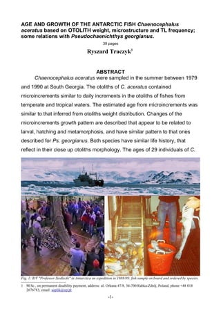
  • 1. AGE AND GROWTH OF THE ANTARCTIC FISH Chaenocephalus aceratus based on OTOLITH weight, microstructure and TL frequency; some relations with Pseudochaenichthys georgianus. 39 pages Ryszard Traczyk1 ABSTRACT Chaenocephalus aceratus were sampled in the summer between 1979 and 1990 at South Georgia. The otoliths of C. aceratus contained microincrements similar to daily increments in the otoliths of fishes from temperate and tropical waters. The estimated age from microincrements was similar to that inferred from otoliths weight distribution. Changes of the microincrements growth pattern are described that appear to be related to larval, hatching and metamorphosis, and have similar pattern to that ones described for Ps. georgianus. Both species have similar life history, that reflect in their close up otoliths morphology. The ages of 29 individuals of C. 1 M.Sc., on permanent disability payment, address: ul. Orkana 47/8, 34-700 Rabka-Zdrój, Poland, phone +48 018 2676783, email: soplik@op.pl. -1- Fig. 1: R/V "Professor Siedlecki" in Antarctica on expedition in 1988/89; fish sample on board and ordered by species.
  • 2. aceratus were determined by microincrements. The age of fish sampled by the fishery (Fig. 1) was predicted from otolith weight using a regression equation. In the other way the age of fish was determined from otolith weight frequency and its modal progress analysis. The results from those methods were compared to each another through the study of spawning, hatching and metamorphose marks in otolith, by back calculating procedure, by length frequency analysis and by comparison with the literature. For C. aceratus the von Bertalanffy growth parameters were, k = 0.26, L∞ = 75, t0 = 0.51. Otoliths size at age, with corrected variability for 3 dimension were established, Tab. 3. INTRODUCTION Chaenocephalus aceratus like other Channichthyidae is a cold adapted fish living exclusively in Antarctic waters. They have low metabolism, prolonged oogenesis, delayed maturation, slow growth, large yolky eggs and iteroparity. Larval stages hatch at large size and at a relatively advanced stage of development. Reproductive cycles appear to be closely linked to the production cycle so that young develop during period elevated production[10] . Channichthyidae have no red blood cells or any oxygen binding pigment. In part compensation directed to increase oxygen respiration are: large head and fins. C. aceratus is distributed in Bouvier Island, islands of the Scotia arc (South Georgia, South Sandwich, South Orkney, and South Shetland Islands) and the Antarctic Peninsula in range of depth from 5 to more 770 m[3] . In the South Georgia - most numerous, in South Orkneys and in the South Shetlands less numerous. There is a succession of species hatching throughout winter to summer at South Georgia. The order of hatching was familial - a bathydraconid then channichthyids, followed by the nototheniids. Their feeding periods are likely to be broadly synchronized with the life cycles of their food species. Their food may be limiting the amount of larvae which can coexist in the ecosystem at any given time of year. Clarke (1988)[9] postulated that production (growth and reproduction) of polar marine -2-
  • 3. ectoterms is limited not by the temperature but by the food availability and that the seasonality of their growth is linked to their position in the food web. Different life- history stages live at different mean depths and distance from the shore, the diet varied for them (Burchett at all 1983)[2] . The adults usually occupying the deepest waters[9] about eight times numerous between 150 and 250 m depth than upper or lower[12] . Their diet varied during the life cycle, further from the shore adults fed mainly upon mysids and fish (Permitin and Tarverdiyeva 1972[12] ). Inshore juvenile feed mostly on decapods shrimps and fish (Burchett at all 1983)[2] . Postlarval and juveniles' forms were lived in the pelagic zone often with krill[6 ,5] Antarctic fish concentration were located very close to the bottom during the day and dispersed into the water column after dark by the echo sounder[12] . The feeding behaviours as well as habitat varied during their life cycle. Seashore they display a high level of nocturnal activity linked to as much of the benthos is also more active at night. Offshore feeding insensitivity of adults is probably highest during the day as was find for N. rossi by Linkowski and Rembiszewski[6] with assumption of Burchett and other, 1983)[2] . In late summer they in schooling move inshore to 240 m depth, from the shelf areas to spawn (Burchett and other, 1983)[2] . At South Georgia spawning occur over limited time period from the end of February to the end of April. With another data spawning: 1) at South Georgia: from March to May (egg are laid from March to May); length at first spawning - 58.4 cm TL for females and 47.5 cm TL for males; 2) at Elephant I., from May to June; length at first spawning - 57.1 cm TL for females and 45.7 cm TL for males. Chaenocephalus aceratus has a relatively high growth rate, but becomes sexually mature at a relatively large proportion of maximum length. By adopting a strategy of growing rapidly to a large size before reproducing, this species can predate a wide size range of fish and so increase its tropic scope. C. aceratus matures at a relatively large size and would therefore be expected to exhibit delayed maturation but the rapid growth rate of this species compensates and so the age of at maturity falls within the trend observed for other notothenioids[9] . Males mostly are smaller by 101 mm than females. Maximum theoretical length of female is 76.5 and -3-
  • 4. male 58 and is related to the size and age at sexual maturity, that are a half to three- quarters of above data 40 - 50 cm with age of seven for female and six for male[5] . The rate of growth to asymptotic size (K) is related to size and age at sexual maturity (0.17 male; 0.24 female[5] ). Length distribution of C. aceratus shows modes at 18 (21g) and 26 cm (90 g), but for longer fish it become indistinct due to differences between the sexes. There is good agreement between the mean length at age and the modal lengths for first two: 1 – 18 cm and 2 – 26 cm age groups. The other follows as in Tab. 1. Tab. 1: Mean length and weight at age of male and female C. aceratus, after Parkes[11] Age: 1 2 3 4 5 6 7 8 9 ♂♂[cm] 18 26 32.6 38.2 45.3 49.4 50.4 ♂♂[g] 21 90 197 350 641 871 945 ♀♀[cm] 47.4 51.9 57 59.7 61.9 ♀♀[g] 756 1050 1464 1726 1988 There was a significant difference between mean length and weight at age of male and female C. aceratus above age 5, Tab. 1. Males of age 7 were on average nearly 7 cm shorter than females of the same age[11] . Previous age data: juveniles from 26 to 35 cm - III and IV age classes. The spawning and the hatching of the early larvae were probably less dictated by occurrence of immature copepods - common food of early larvae of fish. The Antarctic marine environment is highly seasonal with a strong pulse of production occurring over the summer period and minimum in winter (Clarke, 1988[9] ). The timing of spawning and subsequent hatching of larvae in relation to this annual cycle will largely determine the amount of food available to them. Copepods have a life-cycle that is closely linked to the primary production cycle and their abundance parallels phytoplankton productions with high level for most of the summer period from November to February at South Georgia[9] . In advance of the peak in production cycle C. aceratus as same Antarctic species lay large yolky eggs which hatch the large larval stages during autumn and winter[9] . They survive winter by feeding on the overwintering stages of neritic copepods and thus their life cycles -4-
  • 5. are not directly linked to above mentioned high abundance secondary production. In spring they are able to prey upon larval fish which hatch in this period in addition to feeding on other zooplankton. Therefore hatching early in the season seems to be advantageous to species which are piscivorus as larvae (North and Ward 1989[9] ). C. aceratus eggs are yolky and large between 3.9 - 4.7 mm in diameter, and in consequence the fecundity is low (5 - 9 egg by fish total weight in gram)[9] . They have biennial (two years) process in the development of mature oocytes[10] . Size of ripe eggs is: 4.4 - 4.7 mm in diameter. They are laid demersal at depth of 240 m from March to May. When eggs spawned their development period to hatching is one or two month[2, 9] . C. aceratus have extended hatching period: at Antarctic Peninsula is from August to October; and at S. Georgia, It hatch early - in winter (June - November) have 11 - 17 mm total length (as size of eggs) with large yolk sac (about 50 % of the body mass), that is probably utilized within two months of hatching[9] . Larvae are of apterolarval form, and not especially advanced in overall development, although they are somewhat precious because they can soon feed. They have a better muscle arrangement for cruise swimming than the adults, in which slow muscles are only a minor component of the trunk muscles[9] . As the yolk-sac is absorbed, the larvae commence feeding and this is also a future of Antarctic fish larvae (North and Ward 1989[9] ). Their heads and jaws are large enough, Fig. 2, 13, to feed on the overwintering stages of small copepods, such as Drepanopus forcipatus[9] . Hatching spread to four months period producing larvae in sequence reduces the potential for interspecific competition within the ichthioplankton[9] . First individuals to appear preceded the period of increased copepod abundance (by up to five month) feed on small copepods grow sufficiently large to adopt a piscivorus diet when the larval stages from species that breed later arrive in the plankton[9] . They can feed on high level abundance of copepods in spring and summer. The growth rate of larval C. aceratus of 15 - 40 mm SL was about 0.11 -5- Fig. 2: Chaenocephalus aceratus, larva, 2.1 cm, after North.
  • 6. - 0.16 mm SL per day at the Antarctic Peninsula[12] . There are differences in data, Tab. 2, that could be explained by extended hatch period, as it was stated by Ślósarczyk[12] (early in August hatch larva after 6 months in January could be as 8 cm juvenile). Tab. 2: Published data length during larval development August November-early December January-March cm SL cm SL cm SL 1.5 – 1.8 with yolk sac 1.9 – 4.0 with yolk sac 2.2 – 2.3 with yolk sac – 8.0 3.3 – 5.9 to February The larval length span to metamorphosis ranges up to 80 mm (probably in December? Tab. 2) and is over than a typical tropical fish[9] . They growth to the juvenile stage during six, seven month (juvenile were found in January) and it is long period in compare with weeks or days for temperate and tropical marine fish[9] . In late winter larvae within 5 km of the coast of the island were with large shoals in sublittoral waters (less than 40 m depth)[7] . Near the coast at South Georgia, C. aceratus are in most abundant group of larvae in September (early spring) in compare with other months in which the most abundant are different species[8, 7] . In early spring the number of C. aceratus larvae as piscivorus is about one-tenth[9] . In summer the larvae at South Georgia undertook diurnal vertical migrations, when phyto and zooplankton abundance are high[8, 7] . The family Chaenichthyidae provide difficult in age estimation. The methods based on counting annuli marks in otoliths give some mistrust. They show several mark that difficult interpreted and to relate. Daily increments account can verify them. They can give information on seasonal increase, decrease or lack of growth of fish, and morphological and physiological change and shift like change of environment, metamorphose, maturing, spawning and other. This could calibrate the fishing predict of icefish C. aceratus that were exploited since 1977. Foremost in the elucidation of accurate population dynamics' parameters in fish is the correct -6-
  • 7. estimation of age. So here will be try to assess alternative methods of determining the age of the fish from the otolith by comparing ages based on otolith biometry and morphology (height, mass, otolith shape the last, number of primordia was used by Prof A. Kompowski – personal communication), with those derived from internal microincrements. Some additional data on their relations to one to another will be added. The main objective of the present work was to study daily increments of C. aceratus to show biological data and next compare Ps. georgianus and C. aceratus appearances, life stages, behaviours that determine otolith morphology - Ps. georgianus and C. aceratus have similar otoliths and daily increments. MATERIAL, METHODS The sets of ichthyological data on C. aceratus, Fig. 3, collected during three Antarctic expeditions in 1979 (by Polish sciences, Fig. 1), 1990 (by English - Polish FSA sciences group) and in 1986 in the South Georgia area in the summers were -7- Fig. 3. Champsocephalus aceratus, 58 cm TL, during collecting data: length, weight, sex, maturity.
  • 8. taken into account. The otolith was chosen as the best structure for age determination from the other hard structures of this fish (based on published CCAMLR guidelines). Fish were measured and weighed and their sagittal otolith were removed and stored. Age was determined by length frequency analysis. Age determination from the otolith Otoliths were cleaned with a commercial solution of Clorox (5.25% sodium hypochlorite), washed with water, dried, weighted (accuracy ±0.1 mg). Otolith's microincrements and other features were examined using various methods including, light microscopy with transmitted and reflected light, and scanning electron microscopy (SEM). Age was determined in relation to measurements of the otolith external and internal morphometry. To establish the development of the shape of otolith, changes in microincrements pattern, and their distances from the centre was measured in transverse sections (Fig. 4). Whole dried otoliths of all sizes were embedded in epoxy resin in bars and ground on two parallel sides with carborundum paper (No. 80-800) to reveal the nucleus and then mounted in Eukitt (microscopic mounting medium) directly on microscopic slides, Fig. 5, 6. These were ground and polished with a 1 µm diamond compound by hand and grinding machine under water to the thickness of 0.1-0.15 mm to view the microincrements. Sections were released from Eukitt with chloroform -8- Fig. 4: Otolith C. aceratus M-S plane Tplane R 0 1 2 3 mm Fig. 5: Otoliths embedded in resin and mounted on slides. Numbers were draw by diamond on glass, glasses are not show in all ranges. 0 1 2 3 4 5 6 7cm
  • 9. or xylene. Growth pattern from the polished sections were measured. This included recording the width and position of each microincrement and opaque and hyaline zones from centre of the otolith to the edge. Etched sections. To reveal incremental patterns in the surface relief of some polished sections they were etched for 1 - 8 minutes with EDTA. This was on both sides for C. aceratus because their microincrements were visible in light microscope when the both sides of otolith slides were etched. They were cleaned with water and dried. The etched surface was pressed into acetone soaked acetate sheets paper to produce acetate replicas. Dried acetate replicas were photographed. Etched otoliths were coated with a nano- thickness of gold using an electric arc current at an angle of 45º in a vacuum (9.4·10-8 Tr). They were examined by reflected light microscopy. The growth pattern was observed - the positions of ditches created by removing of calcium and corresponding to micro-opaque zones in polished sections, were photographed. Etched and coated otoliths were also examined by scanning (SEM). Microscopic slides, Fig. 5, 6, with one or more coated otolith sections were attached to custom made SEM stubs (the metal plate of the slides size were welded to standard stubs with the connecting metal string to the coated surface), Fig. 7. SEM screen projections of the coated otolith sections were photographed to produce their film negative for further analysis and to -9- Fig. 6: Preparing otoliths from larvae and postlarvae, glasses are not show in all ranges 0 1 2 3 4 5 6 7cm Fig. 7: preparing sample to SEM coated glass surface with gold put connect metal metal
  • 10. microincrements counts by direct measure and count from photograph. The micro- opaque zones appeared dark maxima on the negatives. Age differentiation based on otolith morphology. The parameters of otolith surface morphology were analysed in relation to the fish and otolith size to examine changes in otolith shape during growth. Analysis of the otolith size. The otolith sizes (their limits on the T planes, otolith weight) were analysed by age. Means, variances and standard deviations of the measurements were compared and tested for differences. Back calculations. Assumed little individual variability in the otolith size age relationship permitted the prediction of past growth from the otolith size. Past growth was predicted from the linear regression model of the size of otolith and fish total length relationship. Age determination from otolith weight. The Bhattacharya method[3] was applied to determine age from otolith weight frequency. The left skewness: values on left that are less then mean of groups in the otolith weight frequency were linearised and fitted by the normal distribution whose digits as first age group were subtracted. From remained data its new left skewness were analysed as above to get second age group and after that next older ones. To that age group in otolith ordered weight data (usual 4 groups) their appropriate data fish length data were then taken by that age group. Obtained length frequency of 3 - 4 age group in this way were basis to take into account Bertalanffy growth formula (growth of fish from first to second and next age group) to additional approximate the mean of age group and then to fit correct distribution of age groups in otolith weight frequency and length frequency. Estimate the age of the largest samples. Otolith morphometry were related to age. The relationship between otolith weight and age were used to extrapolate the ages of the largest fish. Where, ages in days were determined by counting microincrement. -10-
  • 11. Analysis of otolith weight frequency at age modes for year sample. The frequency distributions of the measure variables were examined from the larger 3 year sample to detect modes associated with individual cohorts (year- classes). Only data for one season of the year was used. The mean and the standard deviation of otolith parameters of that cohort were examined for variation within and between cohorts by years. The progression of modes in the otolith weight frequency during ontogenesis was analysed to separate age groups and derive growth age groups. The mean size of each age class derived from polymodal frequency analysis of otolith weight was statistically compared (using Least Significant Difference test[1] ). And where they agreed a combined age was produced. Age determination from length frequency. Age determination by Bhattacharya method. The length frequencies were taken from 3 year sample. The left skewness in the length frequency (values on left that are less then mean of group in the TL frequency) were linearised and fitted with the normal distribution. Then the digits as first age groups were subtracted. From remained data its new left skewness were analysed as above to get second age group and after that next older ones. To that age group in fish length the Bertalanffy growth formula was fitted, from which the mean of further age group were predicted. Based on obtained averages of older fish and remained modal frequencies at age (after subtraction frequency of younger age group) the frequency of older fish were estimated and corrected formulas of Bertalanffy equation were then established (on means of age groups). Analysis the progression of age modes during ontogenesis. Sequences of length composition at annually progressing one age group were analysed throughout ontogenesis to get information on the annual growth rate of population of one this same age. Difference among the years were subject to estimate and predict the annually changes in averages of length and in numerous of fish to the stock predict. Fish growth parameters -11-
  • 12. The Bertalanffy growth model[4] was fitted to each set of age data from each method of age determination. Age data was transformed to catch frequency by the Gulland[4] equation: (NiPij) to age at length of the catch frequency, where Ni is the number of fish in i-th. Length class from catch length measure in the season, the Pij is the following proportion: Pij = nij/ni (ni - the number of fish in i-th. length class; nij - the number of fish in i-th. length class and in j-th. age groups). Then they were used to calculate theoretical growth of fish using the von Bertalanff'y equation. Age data were arranged as available cached set of age groups within one season, that were simplify to within one age population during it ontogenesis. RESULTS The growth zones of otolith Daily zones With sectioning and polishing there were micro increments visible. Otolith sections of 29 individuals viewed by the light microscopy showed incremental patterns that were measured and counted (Fig. 9). The manner of increments was observed also on acetate replicas and with SEM, Fig. 8. In the central area of otolith, daily increments were wider, and mostly had 2.5- 4 μm – at distance ~0.002 mm from the centre, Fig. 10, 11. At distance ~0.06 mm daily increments were relatively similar: 2-3.3 µm. But at outer layers up to 0.7 mm distance from the center, increments were very narrow: 1.1-2 µm. At larger distance from the center, the widths of daily increments were alternately wide follow after the small and after them wide again. Apart from that wide – small – wide alternate pattern the increments' width decreasing from the center to the otolith edge in general: at 0.83 mm from the center increments were 2-2.5 µm wide; at 1.43 mm from the center there were 1.29 µm wide; at 2.15 mm there were 1.1-1.25 µm. In average for specified distance from the center there were 3 up to 9 daily increments per 10 µm. That unit was useful for correcting data for adequate sectors with partially destroyed surfaces. -12-
  • 13. -13- Fig. 8: SEM microphotograph of otolith daily increments of C. aceratus.
  • 14. -14- Fig. 9: Microincrements from the transverse section of a sagittal otolith from 45 cm TL C. aceratus applied to daily increment count. From central primordium, CP to the otolith edge there are 1590 days. C B 1590 incr., 2.347 mm 554 incr., 0.816 mm 48 incr., 0.046 mm +1036 incr. +506 incr. +48 incr. CP Ch. aceratus, 45 cm SL, ♀ catch No 136 (sample 75) S. Georgia I. 29.III.1979. Transverse section otolith dorsal area OW=0.024676 gram OR=2.347 mm OH=3.44 mm Left saggittal (a) 0.1mm
  • 15. -15- Fig. 10: Daily increments widths along otolith radius for C. aceratus CPwhitep.:(+):0.003206at0.0076mm LN blue p.: (+): 0.001339 mm at 0.0632 mm first dark mark green p.: (+): 0.002125 mm at 0.1461 mm otolith edges yellow p.: (+): 0.001635 mm at 0.4655 mm second dark mark green p.: (+): 0.001897 mm at 0.2319 mm. AP red p.: (+): 0.00154 mm at 0.6755 mm SP magenta p.: (+): 0.001764 at 1.4575 mm otolith edges yellow p.: (+): 0.00171 mm at 1.7824 mm SP magenta p.: 0.001281 mm at 2.367 mm otolith edges yellow p.: average (+): 0.00143 mm at 2.4589 mm otolith edges yellow p.: (+): 0.00242 mm at 1.2183 mm widthincrements=-52.850746·R+0.623567 0.3 0.4 0.5 0.6 0.7 0.2 0.1 0 1.3 1.4 1.5 1.6 1.7 1.2 1.1 0.8 0.9 1.0 1.8 1.9 2.3 2.4 2.5 2.6 2.7 2.2 2.1 2.0 2.8 2.9 3.0 Otolith radius [mm] 0 0.0005 0.001 0.0015 0.002 0.0025 0.003 0.0035 0.004mm: 0.0045 0.02 microincrements width [mm] width of daily increments in 28 otoliths along their radii
  • 16. -16- Fig. 11: The numbers of daily increments along otolith radius in C. aceratus. 6 white p. – set of CP with (+) - an average distance at 0.0076 mm and with 3 days from start 25 blue p. – set of LN with (+) - an average at 0.0632 mm and with about 47 days 3 green p. - set of first dark mark at 0.1461 mm (+) and with 87 days 7 yellow p. - set of otolith edges with (+) - mean radius R ≈ 0.4655 mm and with about 242 days 2 green p. - set of second dark mark at about 0.2319 mm (+) and with about 129 days 7 red p. - set of AP with (+) - an average at 0.6755 mm and with about 472 days 2 magenta p. - set of SP with (+) - an average at 1.4575 mm and with about 755 days 6 yellow p. - set of otolith edges with (+) - mean radius R ≈ 1.7824 mm and with about 1152 days magenta p. - mark of SP at 2.367 mm and about 1699 daily increments 0.3 0.4 0.5 0.6 0.7 0.2 0 200 400 600 800 1000 1200 1400 1600 1800day: 2000 2200 0.1 0 1.3 1.4 1.5 1.6 1.7 1.2 1.1 0.8 0.9 1.0 1.8 1.9 2.3 2.4 2.5 2.6 2.7 2.2 2.1 2.0 2.8 2.9 3.0 5 yellow p. - set of otolith edges with (+) - mean radius R ≈ 2.4589 mm and with about 1578 days 4 yellow p. - set of otolith edges with (+) - mean radius R ≈ 1.2183 mm and with about 523 days Days =733.1621·R[mm]-13.38 Otolith Radius [mm]=0.001227·days+0.0068795 Otolith radius [mm] growth of daily increments in 28 otoliths along their radii
  • 17. The 4 individuals 4 - 9 cm juvenile were have 121 - 250 micro-increments (Fig. 14, 19, 20). As they had not 365 days they were classified as age group 0. Otolith weight = 0.18 – 0.47 mg. OH≈OL=0.53 mm, Tab. 3. The 4 individuals ranged at 18 -24 cm TL, Fig. 12, had 479 - 598 daily increments. Their otoliths were associated with fish group I. Otolith mean = 4.7 mg (increase with 4.3 mg from age 0), Fig. 13. OH=1.72 mm, OL=1.84 mm, Tab. 3. The 4 individuals little larger: 25 -27 cm TL had 931 - 967 daily increments, Fig. 21 and were classified to fish group II. Otolith mean = 9.5 mg (increase with 4.7 mg from age I). OH=2.49 mm, OL=2.73 mm, Tab. 3. Fish of 26-35 cm TL possible age group III in agreement with published data and with TL frequency analysis (lack data on daily increments data). Otolith, Fig. 15, have weight mean = 14 mg (increase with 4.5 mg from age II). OH=3.38 mm, OL=3.94 mm. For the next 9 individuals with average length above 44 cm TL there were 1494-1700 daily increments, Fig. 9, 22. They were classified as age group IV. Otolith, Fig. 16, mean = 23.5 mg (increase with 6.5 mg from age III). Start change -17- Fig. 14: Otolith's T- plane, 8 cm TL; H×L: 0.5×0.5 mm Fig. 12: C. aceratus, 20 cm TL. Fig. 13: Otoliths after Hecht [5] 1.7×1.8 mm 2.5×2,7 mm Fig. 15: Otoliths after Hecht[5] 3.2×4.2 mm H×L 3.6×3.7 mm H×L Fig. 16: Otolith after Hecht [5] 3.4×4.3 mm H×L Fig. 17: Otoliths after Hecht [5] 4.5×4.5; 4.3×5.2
  • 18. growth pattern in the space, Tab. 3. OH=3.44 mm. OL=4.27 mm. The 3 fish ranged 52 – 60 cm TL, Fig. 3, had 2354- 2604 daily increments in their otolith, Fig. 17 that classified as fish age group VI. OH=4.39 mm, OL=4.83 mm, Tab. 3. They should be classified with sex. Larger fish, that have larger otoliths Fig. 18, should be classified as fish age group VII+, OH, OL as in Tab. 3. There are one year differences in the number microincrements developed among otoliths of different size, that become from the stable growth of otolith at all, during fish life, which reflect in stable yearly increase of otolith weight: ~4.7 mg between age class. But otolith growth was not proportionally to the surface of the otolith. From that fish at different age have their own characteristic shapes of otolith that did not change during our sampling period. This is helpful to identify the age (as Prof. Dr A. Kompowski from numbers of hills- primordia of hilly otoliths of C. aceratus: personal communications) and the period life of fish from otolith morphometry measurements and shape, Fig. 13-18. Others marks in increments pattern of otolith in relation to the ageing. A. CP - central primordium, otoliths primer, that with 3-7 daily concentric unit form – small ball with the radius of 0.0076 – 0.0125 mm Fig. 11, 19, 20, 23. CP mark probably indicate the end of develop of embryonic inner ear of fish. Its inner 3 - 7 microincrements may reflect rather embryonic developments stages than daily increments. B. LN – larval nucleus, after next ~44 microincrements is nucleus edge, clear distinguished by oval black mark in profile at ~0.0632 mm from the center, Fig. 11, 19, 20, 23, 24, 25. That mark is the first wide and dark concentric mark surrounding CP. In the central area of otoliths that primer is possible the only one primary point from which the growth of otoliths has been radiated. In the nearest, outside the LN, -18- Fig. 18: Otoliths after Hecht [5]. 4.8×5.9; 5×4.5; 5.1×5.1 mm
  • 19. -19- Fig. 19: C. aceratus otolith (postlarvae) transverse plane showing concentric daily increments, that were chosen for age determination (dorsal area). Ch. aceratus, 7.6 cm SL catch No 62 (sample 18) S. Georgia I. Jan.1990. edge 0.08087 mm 24 incr., 0.0337 mm 0.21 mm 284 incr., 0.3213 mm +17 incr. +114 incr. +146 incr. CP Transverse section OW=0.0003112 gram OR=0.32125 mm Left saggittal (a) 0.1mm 7 incr., 0.0125 mm 138 incr., 0.14375 mm
  • 20. -20- Fig. 20: Microincrements from the transverse section of a sagittal otolith from a 6.3 cm SL C. aceratus, showing larval and postlarvae increments pattern as daily increments count. There are 6 daily sequences in increments pattern. NHM – Nucleus Hatching Mark. +198 incr. +20 incr. +38 incr. 256 incr., 0.3972 mm 20 incr., 0.0175 mm 58 incr., 0.06674 mm CP Ch. aceratus, 6.3 cm SL, catch No 26 (sample 5a) S. Georgia I. Jan.1990. Transverse section otolith dorsal area OW=0.000191 gram OR=0.397 mm OH=0.77 mm Left saggittal (a) 0.1mm NHM
  • 21. -21- Fig. 21: C. aceratus otolith (27 cm SL) showing microincrements as utilized as daily increments account. Transverse section, dorsal area. 4.5 Ch. aceratus, 27 cm SL, ♀ catch No 136 (sample 42) S. Georgia I. 29.III.1979. AP SP 217 incr., 0.443 mm H G F E D B C edge A 1 A 2 142 incr., 0.308 mm 290 incr., 0.603 mm 351 incr., 0.761 mm 382 incr., 0.828 mm 767 incr., 1.488 mm 967 incr., 1.86 mm 122 incr., 0.263 mm 74 incr., 0.163 mm25 incr.; 0.033 mm +20 incr. +75 incr. +73 incr. +61 incr. +31 incr. +385 incr. +200 incr. +48 incr. +49 incr. +25 incr. CP Transverse section otolith dorsal area OW=0.009543 gram OR=1.86 mm Left saggittal (a) 0.1mm
  • 22. -22- Fig. 22: C. aceratus otolith (43 cm SL) showing microincrements as utilized as daily increment account. Transverse section dorsal area. Ch. aceratus, 43 cm SL, ♀ catch No 136 (sam. 73) S. Georgia I. 29.III.1979. AP 134 incr., 0.176 mm edge 512 incr., 1.005 mm 1011 incr., 1.935 mm 1648 incr., 2.338 mm 54 incr., 0.073 mm +80 incr. +378 incr. +499 incr. +637 incr. +54 incr. CP Transverse section otolith dorsal area OW=0.023169 gram OR=2.338 mm Left saggittal (a) 0.1mm
  • 23. -23- Fig. 23: Microincrements in the central nucleus area, from the transverse plane of a sagittal otolith of C. aceratus. Ch. aceratus, 7.6 cm SL catch No 62 (sample 18) S. Georgia I. Jan.1990. 24 incr., 0.0337 mm CP Transverse section otolith central area OW=0.0003112 gram OR=0.32125 mm Left saggittal (a) 0.1mm 56 incr., 0.0809 mm+32 incr., +24 incr.,
  • 24. -24- Fig. 24: Numbers of daily increments in otolith of C. aceratus. 0 1 2 3 4 5 6 7 8 9 10 11 12 13 5 7 9 11 13 15 17 19 21 23 25 27 29 31 33 35 37 39 41 43 45 47 49 51 53 55 57 59 61 63 65 67 cmTL: Numbers Juveniles Sex 2 Sex 1 C. aceratus from S. Georgia I, March, 29-30 1979; Catch: 136, 139; N=202; 34720.04508 00 0 1 2 3 4 5 6 7 8 9 10t: 0 1 2 3 4 5 6 7 8 9 0 10 20 30 40 50 60 70 TL, cm 0 366 731 1097 1462 1828 2193 2559 2924 3290 3655 days 366 731 1097 1462 1828 2193 2559 2924 3290 183 548 914 1279 1645 2010 2376 2741 3107 183 548 914 1279 1645 2010 2376 2741 3107 0 0.00208 0.00714 0.0122 0.01726 0.02231 0.02737 0.03243 0.03749 0.04255 0.04761 gram 0.00104 0.00461 0.00967 0.01473 0.01978 0.02484 0.0299 0.03496 0.04002 0.00103 0.00813 0.01524 0.02234 0.02944 0.03654 0.04364 0.05074 0.05784 0.00051 0.00458 0.01168 0.01879 0.02589 0.03299 0.04009 0.04719 0.05429 Lt =75(1-e-0.18(t-0.06)) Lt =75(1-e-0.26(t-0.51)) t[y]=140.82·OW[g]+0.8546t[y]=197.64·OW[g]+0.5898 7 12 17 22 27 0 0.5 1 1.5 2 2.5 3mm 0 0.005 0.01 0.015 0.02 0.025 0.03g d[mm]=-0.000135·R[mm]+0.002018 d[mm]=-0.018721·OW[g]+0.002009 d[·10-4mm] R=otolith radius; OW=otolith weight d=width of daily microincrements in otolith OW[g]=-0.010111·R[mm]-0.004532; R[mm]=-85.046·OW[g]+0.58285 Age[years]=1.785594·R[mm]-0.264411 TL[cm]=15.226·R[mm]+3.243 0 0.5 1 1.5 2 2.5 3 70 10 20 30 40 50 60 TL, cm 7 1 2 3 4 5 6 Age [years] 0 22 32 42 52 62 72 LN, days, years LN[days]=414.1834·RLN[mm]+20.2666 0.02 0.03 0.04 0.05 0.06 0.07 0.08 0.09 0.1 0.11 RLN[mm]=0.000818·LN[days]+0.02546 Age[years]=140.81739·OW[g]+0.854569 Age[years]=390.42433·OW[g]+0.509984 0.0001 0.0002 0.0003 0.0004 0.0005 0.0006 .3 0.4 0.5 0.6 0.7 0.8 0.9 1 122 183 244 305 366 years days Age[y]=197.63679·OW[g]+0.589768 Otolith Weight [g] =0.001163 R[mm]-0.000221 juveniles adults Daily increments count0.09 0.12 0.14 0.17 0.2 0.06 Nucleus Radius [mm] Otolith Radius [mm]=834.90666·OW[g]+0.197463 0.281 0.365 0.448 0.531 0.615 0.698
  • 25. -25- Fig. 25: Numbers of daily increments in otoliths (juvenile, young fish). Age[y]=0.214·TL[cm]-1.155 TL[cm]=0.21381·Age[y]+8.167599 0.52 0.57 0.62 0.67 0.72 0.77 0.82 0.87 0.92 0.97 3.5 4.5 5.5 6.5 7.5 8.5 9.5 190 208 227 245 263 281 300 318 336 355d: y: 0.005615 0.005868 0.006121 0.006374 0.006627 0.00688 0.007133 0.007386 0.007639 0.007892[g] Age[y]=140.8·OW [g]+0.86 Age[y]=390.4·OW [g]+0.51 Age[y]=197.6·OW [g]+0.59 forjuveniles only Daily increments count TL, cm Lt =10(1-e-32.08(t-0.58)) Lt =10(1-e-16.24(t-0.49)) Lt =10(1-e-45.02(t-0.85)) 0.0001 0.0002 0.0003 0.0004 0.0005 0.0006 0.0007 Otolith Weight [g] =0.001163 R[mm]-0.000221 Otolith Radius [mm]=834.90666·OW[g]+0.197463 0.3 0.4 0.5 0.6 0.7 0.2 meanpositionofseconddark mark:0.2319mm;129days meanpositionofCP:0.0076mm;3days 0 100 200 300 400 500 600 700 800 900 day 0.3 0.4 0.5 0.6 0.70.20.10 0.8 0.9 meanpositionofLN:0.0632mm;47days meanpositionoffirstdarkmark: 0.1461mm;87days meanradiusofotolithedges: R≈0.4655mm;242days meanpositionofAP: 0.6755mm;472days Days =733.1621·R[mm]-13.38 Otolith Radius [mm]=0.001227·days+0.0068795 yellow p. - otolith edges; red p. - AP otolith radius [mm] growth of daily increments in 28 otoliths along their radii 0 0.5 1 1.5 2 2.5 3 3.5 4 20 ·10-3mm10 5 2nddarkmark:0.001897mm CP:0.003206mm LN:0.001339mm 1stdarkmark:0.002125mm otolithedge:0.001635mm AP:0.00154mm 0.3 0.4 0.5 0.6 0.70.20.10 0.8 0.9 otolith radius [mm] width increments =-52.850746·R+0.623567 width of daily increments in 28 otoliths along their radii 0 100 300 500 700 900 1100 1300 1500 1700 days 0.4 1 1.5 2 2.5 3 Days =733.1621·R[mm ]-13.38 otolith radius [mm] Daily increments in 32 otoliths along their radii
  • 26. there were possible other similar ones from which further growth of otoliths is going parallel in time into the other directions and resulting as for example the anterior or posterior collicula, Fig. 17, or another otolith's surface hills, Fig. 13-18. C. Nucleus hatching mark (NHM). Next visible circle dark check follow at ~0.1461 mm distance from CP with ~40 daily increments from the LN (nucleus core), Fig. 11, 19, 20, 23, 24, 25. That mark is the second wide and dark concentric mark from the center That dark zone marks the end of discoid nucleus (Fig. 23). Its inner microincrements radiated from CP edge were very clear and regular – so there were possible daily increments and indicate the start of full function of larval inner ear. This mark were accepted as hatching mark (HM) based as described that egg larva develop main tissues and organs ready to seem and feed at hatching in strong Antarctic environment. Yolk sac larvae of C. aceratus after hatching have that organs advanced developed in compare to other species. Because of that they should have a clear otolith increment. Descriptions these structures are in [2]. As the egg larva had developed its main tissues ready to swimming, and feeding at time hatching[2] , the inner ear with otolith should be as well. That advanced body develop of larva should be happen not only in 47 days of larval nucleus, but during additional a month growth (40 days) with the ending as NHM being over in otolith microstructure. From published data is that when eggs spawned (eggs are laid demersal at depth of 240 m, over a limited time period from March to May) their development period to hatching is one or two month (Burchet at all 1983 in [9]). This is agreeing with assumption that 40 microincrements of the NHM, as previous 47 of LN, were deposited during larval develop in the egg. 2.3 cm larvae of C. aceratus have yolk sac, reaches in organic matrix, so growth of larval otolith should not be restricted. It could be possible to find numbers of days of otolith growth for larvae from otolith increments. Otolith 0.1683 mg growth to 0.3142 mg during 284-144=140 days, this means 0.001042 mg per day. From that otolith 0.18 mg is growth for at least 0.1683/0.001042=162 days, not 3-47 days of LN. D. First accessory primordium (AP). Postlarvae mark of 0 age class in otoliths. First changes in pattern increment at the edge of larger otoliths of younger fish were -26-
  • 27. followed after ~ 472 increments about ~0.6755 mm from the center to the dorsal area, Fig. 9, 10, 11, 21, 22, and 25, In the larger otolith of older fish it is shown in this same manner versus the otolith center The microincrements following the AP were propagated along a new growth axis with at an angle of ~30° to thus far otolith growth radius. When only the start of AP is in otolith, this means when AP were not hinted by outer layers, then this classify the fish into 0 age class (or postlarvae with completed 1 year age and at the beginning of I age class). When AP was overlying then this classify fish into I age class. This well agree with otolith dorsal radius equal to 0.465 mm from juveniles age class 0 caught in January (add 90 increments per 0.1 mm giving value comparable with otolith radius of 0 age class fish cached in March, 30). It is possible to relate above mark of AP to the adequate period of change environments habitats that associate to the period time with shift from postlarvae to adult. E. Second accessory primordium (SP). Juvenile mark of I age class in otoliths. Second similar to AP change in pattern microincrements was placed further 385 daily increments and 0.66 mm from AP, this means at 0.66+0.675=1.355 mm distance from the CP to the dorsal margin direction, Fig. 9, 10, 11, 21, 22, 25. From origin of SP, the deposition of otolith matrix follows in different manner: daily increments were darkness (possible more calcified) grouped in sequences and into pattern of vowels. Like mark of AP, the SP marks fish in age class I in agreement with dorsal radius 1.19-1.3 mm in otolith classified (by number of daily increments) into I age group. SP indicate an annual growth otoliths with start the deposition of otoliths matrix from dorsal edge of otoliths of fish in I age class. This mark may be related with adequate period of maturing of fish. F. Two and tree annuli marks. In dorsal area of larger otoliths after juvenile marks a few similar to them were find. The distance between them were approximately two and three annuli in amount of daily increments. Those marks may be related with first and further spawning periods. Adults have biennial (two years) process in the development of mature oocytes[10] . The development of mature ova takes two years at South Georgia Island (Kock, 1979 after Burchett[2] ). -27-
  • 28. Some relationship of changes in microincrements pattern with biology and environment We can treat CP (richest in organic matrix) as mark of the start of embryonic development and AP as a start of postembryonic development that have: juveniles and also sexually mature adults and fish in senescescent phase as well. Both CP and AP, SP seems to have similar process in forming, with a little difference in environment. CP radiate to ball, so in all direction that is possible when it is processing only in liquor of inner ear. Start AP and SP is happen on otoliths surface that restrict otoliths growth radiate in liquor into only one side, but the nature of it is the same. Postlarvae start the metamorphose process and move from pelagic to demersal zone probably in March. They have vertical migration as their food undergo. This may determine easy choose the life style to deeper waters as some different environment conditions of pelagic and demersal zones were explored by postlarvae during their vertical migrations. Environment conditions have very strong influence on fish life and strategy. So as the AP is a large change in otolith microstructure it seems to be associated with metamorphose process. Biology and age. 4-9 cm TL postlarvae were caught in January and as they had from hatching mark to otolith edge ~100-200 daily increments, or ~3-7 months, they hatch from June (Jan.-7 months) to October (Jan. - 3 months). Published hatching period at Antarctic Peninsula is August-October so at S. Georgia hatching period should occur from June to August in agreement with published information that at S Georgia spawning period was taken 3 month earlier, than it undergo farther to South. This -28- Fig. 26: Compare age reading (under line) with published hatching periods. II III IV V VI VII VIII IX X XI XII I II III S. Georgia I. Elephant I. Antarctic Penninsula Spawning Extended hatching Hatching 1.5-1.8 cm SL 1.9-4 cm SL 3.3-5.9 cm SL 9.3 cm SL4-8S. Georgia I. Publisheddata Age: 144-284 days ? Month: Hatching ?
  • 29. similar relation may be applied to a hatching, Fig. 26. Period of hatch: June to October - taken from position of hatching marks, including above interpretation of published data, is in agree with Ślósarczyk's[12] opinion: that C. aceratus hatch during extended period. Also as postlarvae growth fast, this same is for their otoliths, which increase 2.6 times over 3 months: from 0.168 mg in January to 0.47 mg in March. Similar next separate group of larger fish: 18-24 cm TL classified to I age group, that is in agree with published data have the number of daily increments and CP position, that pointed hatch period into September, October. All daily increments age data - t, had well linear dependence from otolith weight, OW[g]: t=140.82·OW+0.8546, Fig. 27. Follow that relationship, from otolith weight age of all fish was estimated. Using L∞=75 cm TL (the largest fish), mathematic formulas for K, t0, growth of fish was derived: Lt=75(1-e-0.26(t-0.51)), Fig. 28. To compare above result, to give up the daily increment account, separate groups from otolith weight frequency, were chosen to which age class were wrote, and next linear regression, as above, and finally Bertalanff’y growth formula, the same as above: Lt=75(1-e-0.26(t-0.51)), Fig. 28. In additional length fish data were divided to the age group by Bhattacharya method, Fig. 28, 29. In this method fish growth equations were obtained, for each sample different, for 1979: Lt=75(1-e-0.253(t-0.562)); for 1990: Lt=75(1-e-0.216(t-0.568)); for 1992: Lt=75(1-e-0.172(t-0.137)), Fig. 28, 29. In above material, there were alternative different interpretation of data, that have source probably from rather sex difference, then age difference (more number age groups), but instead of that, separate sex data for 1979, were well explained by one following equation: Lt=75(1-e-0.26(t-0.51)), Fig. 29. -29-
  • 30. -30- Fig. 27: Otolith weight groups OW:0.000257(s=0.0001158)g TL:8.06(s=0.96)cm;N=25 0 10 20 30 40 50 60 70 6 2 4 3 5 1 7 0 10 8 9 25 0 OW:0.004554(0.0003841)g TL:20(1.67)cm;N=5 0.009812(0.0006583)g 26.7(1.42)cm;N=30 0.014876(0.0013117)g 33.5(2.09)cm;N=32 0.020592(0.0015733)g 41.5(4.82)cm;N=12 0.024813(0.0015551)g 45.5(2.86)cm;N=23 0.029379(0.0007253)g 51.1(2.93)cm;N=8 0.034967(0.001861)g 55.1(4.01)cm;N=40 0.040521(0.000918)g 59.9(3.57)cm;N=18 0.044673(0.0015517)g 61.8(4.60)cm;N=6 0.049022(0)g 63(0)cm;N=1 0.055003(0)g 66(0)cm;N=1 diff.:~0.00348g diff.:~0.00358g diff.:~0.00091g diff.:~0.00107g diff.:~0.00055g diff.:~0.00059g diff.:~0.00095g diff.:~0.00076g diff.:~0.00093g diff.:~0.00176g diff.:~0.00598g 1.77·10-5g 2.81·10-4g 7.5·10-5g 1.52·10-4g 4.1·10-4g 2.31·10-4g 3.22·10-4g 1.71·10-4g 2.04·10-4g 1.02·10-3g TL, cm I II III IV V VI VII VIII IX X XI Lt =75(1-e-0.18(t-0.06)) t=197.64·OW[g]+0.5898 OW:0.000257(s=0.0001158)g TL:8.06(s=0.96)cm;N=25 0 10 20 30 40 50 60 70 0.00054 0.00006 0.00103 0.00151 0.00248 0.00199 0.00296 0.00344 0.00441 0.00393 0.00489 0.00538 0.00634 0.00586 0.00682 0.00731 0.00827 0.00779 0.00876 0.00924 0.01021 0.00972 0.01069 0.01117 0.01214 0.01166 0.01262 0.01311 0.01407 0.01359 0.01456 0.01504 0.01600 0.01552 0.01649 0.01697 0.01794 0.01745 0.01842 0.01890 0.01987 0.01939 0.02035 0.02084 0.02180 0.02132 0.02229 0.02277 0.02374 0.02325 0.02422 0.02470 0.02567 0.02518 0.02615 0.02663 0.02760 0.02712 0.02808 0.02857 0.02953 0.02905 0.03002 0.03050 0.03147 0.03098 0.03195 0.03243 0.03340 0.03292 0.03388 0.03437 0.03533 0.03485 0.03581 0.03630 0.03726 0.03678 0.03775 0.03823 0.03920 0.03871 0.03968 0.04016 0.04113 0.04065 0.04161 0.04210 0.04306 0.04258 0.04355 0.04403 0.04499 0.04451 0.04548 0.04596 0.04693 0.04644 0.04741 0.04789 0.04886 0.04838 0.04934 0.04983 0.05079 0.05031 0.05128 0.05176 0.05273 0.05224 0.05321 0.05369 0.05514 0.05417 0.05666 6 2 4 3 5 1 7 0 10 8 9 25 0 OW:0.004554(0.0003841)g TL:20(1.67)cm;N=5 0.009812(0.0006583)g 26.7(1.42)cm;N=30 0.015282(0.0016872)g 33.8(2.65)cm;N=36 0.025096(0.0028133)g 46.3(3.83)cm;N=39 0.034967(0.001861)g 55.1(4.01)cm;N=40 0.040521(0.000918)g 59.9(3.57)cm;N=18 0.045294(0.0020929)g 62(4.28)cm;N=7 0.055003(0)g 66(0)cm;N=1 diff.:~0.00348g diff.:~0.00358g diff.:~0.00091g diff.:~0.00181g diff.:~0.00095g diff.:~0.00064g diff.:~0.00093g diff.:~0.00598g 1.77·10-5g 2.81·10-4g 7.5·10-5g 2.25·10-4g 2.85·10-4g 1.71·10-4g 2.44·10-4g 1.63·10-3g TL, cm I II III IV V VI VII VIII Lt =75(1-e-0.26(t-0.51)) t=140.82·OW[g]+0.8546 class width = 0.000483165 g C. aceratus from S. Georgia I, March, 29-30 1979; Catch: 136, 139; N=202; OW frequency; 113 class [g]; t=ā for OW groups Lt =75(1-e-0.18(t-0.06))Lt =75(1-e-0.26(t-0.51)) t=140.82·OW[g]+0.8546 t=age means for OW groups t=197.64·OW[g]+0.5898 0 I II III IV V VI VII VIII IX X XI IV V VI VII VIII [gram] 0 1 2 3 4 5 6 7 8 9 10 11 12 13 14 18 0 2 4 6 8 10 12 16 Age,years 5 7 9 11 13 15 17 19 21 23 25 27 29 31 33 35 37 39 41 43 45 47 49 51 53 55 57 59 61 63 65 67 cmTL: Numbers 0 1 2 3 4 5 6 7 8 t=age,years t=140.82·OW[g]+0.8546 age means for OW groups t=197.64·OW[g]+0.5898 Number of daily increments Regression for first 5 circles: Regression for 6 crosses age means for extended OW groups 366 732 1098 1464 1830 2196 2562 2928 t=age,days t=143.86·OW[g]+0.9788Regression for first 7 circles: similar to regression for daily increments.
  • 31. -31- Fig. 28: Age groups by Bhattacharya method. 70 0 10 20 30 40 50 60 1 2 3 4 5 6 7 8 9 0 0.01 0.02 0.03 0.04 0.05 0.0578 Lt =75(1-e-0.26(t-0.51)) t[y]=140.82·OW[g]+0.8546 TL, cm Males catch No 139 1 2 3 4 5 6 7 8 9 0 0.01 0.02 0.03 0.04 0.05 0.0578 Lt =75(1-e-0.26(t-0.51)) t[y]=140.82·OW[g]+0.8546 Females catch No 139 0 ,0 0 4 0 , 0 0 5 0,0 0 Lt =75(1-e-0.172(t-0.137)) Total Length, cm Lt =75(1-e-0.158(t+0.082)) 0 20 30 40 50 60 7010 0 20 30 40 50 60 7010 150 250 300 400 450 500 350 200 100 50 0 -4 -2 -1 2 3 4 1 -3 0 y=-0.77·TL+6.1 y=-0.96·TL+16.97 y=-0.55·TL+14.37 y=-0.12·TL+4.19 y=-0.21·TL+8.42 y=-0.46·TL+21.08 y=-0.56·TL+27.83 y=-0.85·TL+44.51 y=-0.37·TL+20.54 y=-0.66·TL+39.15 y=-0.79·TL+49.19 y=-2.44·TL+158.48 y=-1.08·TL+72.4 (y=0;TL=7.92cm) (y=0;TL=17.76cm) TL=26.14cm TL=34.54cm TL=40.4cm TL=46.01cm TL=49.56cm TL=52.39cm TL=55.76cm TL=59.34cm TL=62.52cm TL=64.96cm TL=67.34cm 2.63 4.63 5.63 7.63 8.63 9.63 6.63 3.63 1.63 0.63 10.63 11.63 12.63 N=29 N=626 N=1587 N=843 N=186 N=218 N=142 N=89 N=102 N=120 N=56 N=21 N=11 y=lnNx+1-lnNx Numbers Age,years C. aceratus from S. Georgia I, January, 3-30 1992 K=(1/(t2-t1))ln((L∞-L1)/(L∞-L2))=0.158 t0=t1+(1/K)ln(1-L1/L∞)=-0.082 1 1.5 2 2.5 0.5 0 y=-0.172·t-0.024 y=-0.158·t+0.013 t0=-0.024/0.172=-0.137 K=b=-0.172 t=age, [years] y=ln(1-TL/L∞) 0 2 3 4 5 6 71 8 9 11 13 C. aceratus from S. Georgia I, March, 30 1979 Jan1990 70 0 10 20 30 40 50 60 1 2 3 4 5 6 7 8 9 0 0.01 0.02 0.03 0.04 0.05 0.0578 Lt =75(1-e-0.26(t-0.51)) t[y]=140.82·OW[g]+0.8546 TL, cm Males catch No 136 1 2 3 4 5 6 7 8 9 0 0.01 0.02 0.03 0.04 0.05 0.0578 Lt =75(1-e-0.26(t-0.51)) t[y]=140.82·OW[g]+0.8546 Females catch No 136 C. aceratus from S. Georgia I, March, 29 1979
  • 32. -32- Fig. 29: Age groups by Bhattacharya method from 2 seasons. Lt =75(1-e-0.253(t-0.562)) Lt =75(1-e-0.183(t-0.0723)) 0 20 30 40 50 60 7010 8 10 12 14 6 4 2 0 2.79 4.79 5.79 7.79 8.79 6.79 3.79 1.79 0.63 N=29 N=6 N=38 N=39 N=29 N=40 N=5 N=7 Numbers Age,years C. aceratus from S. Georgia I, March, 29-30 1979; catch No: 136, 139. N=32 Total Length, cm 1 1.5 2 2.5 0.5 0 0 2 3 4 5 6 71 8 9 y=-0.253·t-0.142 y=-0.183·t-0.0133 t0=-0.0133/0.183=-0.0723 t0=-0.142/0.253=-0.562 K=b=-0.253 t=age, [years] y=ln(1-TL/L∞) 0 20 30 40 50 60 7010 -4 -2 -1 2 3 4 1 -3 0 -5 y=-0.77·TL+6.1 y=-0.41·TL+8.92 y=-1.03·TL+28.41 y=-0.24·TL+8.14 y=-0.24·TL+10.98 y=-0.36·TL+19.18 y=-0.2·TL+12.1 y=-2.44·TL+157.09 y=-0.44·TL+29.29 (y=0;TL=7.92cm) (y=0;TL=22cm) TL=27.69cm TL=34.61cm TL=45.23cm TL=52.82cm TL=60.04cm TL=64.27cm TL=66.62cm y=lnNx+1-lnNx Jan1990 Lt =75(1-e-0.216(t-0.568)) Lt =75(1-e-0.172(t-0.152)) 0 20 30 40 50 60 7010 40 50 60 80 30 20 10 0 70 2.63 4.63 5.63 9.63 10.63 8.63 3.63 1.63 0.63 7.63 6.63 N=29 N=75 N=248 N=211 N=62 N=48 N=9 Numbers Age,years C. aceratus from S. Georgia I, January, 1990 N=72 Total Length, cm N=20 N=55 N=3 Jan1990 (y=0;TL=16.82cm) 0,00 0 20 30 40 50 60 7010 -2 -1 2 3 1 -3 0 y=-0.77·TL+6.1 y=-3.02·TL+50.87 y=-0.75·TL+19.59 y=-0.13·TL+4.29 y=-0.11·TL+4.64 y=-0.12·TL+5.72 y=-0.59·TL+30.49 y=-0.38·TL+21.31 y=-0.22·TL+13.27 (y=0;TL=7.92cm) TL=26.03cm TL=33.5cm TL=41.02cm TL=46.97cm TL=52.08cm TL=56.37cm TL=59.89cm y=lnNx+1-lnNx y=-0.2·TL+13.44TL=66.28 y=-0.73·TL+49.44TL=68.02cm K=(1/(t2-t1))ln((L∞-L1)/(L∞-L2))=0.172 t0=t1+(1/K)ln(1-L1/L∞)=-0.152 10 2 3 4 5 6 7 8 9 1110 y=-0.216·t-0.123 y=-0.172·t-0.026 t0=-0.026/0.172=-0.152 t=age, [years] y=ln(1-TL/L∞) t0=-0.123/0.216=-0.568 K=b=-0.216 1 1.5 2 2.5 0.5 0
  • 33. DISCUSSION From published data is that C. aceratus hatched at S. Georgia in winter (June - November) have 1.1 – 1.7 cm total length, Fig. 26, with large yolk sac (about 50 % of the body mass), that is probably utilized within two months of hatching[9] . The larval length span to metamorphosis ranges up to 8 cm (probably in December)[9] ). They growth to the juvenile stage during six, seven months (juvenile were found in January)[9] . 6-7 months is 180-210 days and that is not appositive to 4 - 9 cm juvenile that had 144 – 284 daily increments in otolith and classified to 0 age class. Next length and age groups is 18 -24 cm TL in I age class. Juvenile phase - definition published for fish 26 - 35 cm length. Fish under this size 25-27 cm were classified to II age class, by number of daily increments equal to 931 - 967 – which is not 6-7 months. From developed wide range in numbers of daily increments 121 – 250, is that hatch could be a long period, even 6 months. Larval stages were found during long period, Fig. 26. Long period of hatch for icefish was found by Ślósarczyk. Similar for wide spawning period was published, that hatching spread to four month period producing larvae in sequence reduces the potential for interspecific competition within the ichthioplankton and may result in adopting the ways of alternative tropic strategies[9] . First individuals to appear preceded the period of increased copepod abundance (by up to five month) feed on small copepods grow sufficiently large to adopt a piscivorus diet when the larval stages from species that breed later arrive in the plankton[9] . In addition they can feed on other zooplankton, on high level abundance of copepods in spring and summer. The growth rate of larval C. aceratus of 1.5 – 4.0 cm SL was about 0.11 - 0.16 mm SL per day at the Antarctic Peninsula[12] , so there are after 4 months, in January they could have 3-6 cm SL. That is not in opposite to the result that 0 age group at S. Georgia with length ~7 cm SL have not completed a year of life: 144-284 days, at S. Georgia they are larger, as they hatch 2-3 months earlier, they 0.9- 1.5 mm longer from 2-3 months of grow before catch them -33- Fig. 30: Drop in the numbers of larvae for Ps. georgianus but increase for C. aceratus during a time period from winter to summer (May to March).
  • 34. in January, Fig. 26. In late winter larvae within 5 km of the coast of the island were with large shoals in sublittoral waters (less than 40 m depth)[7] . It is suggested that cyclonic currents retain the larvae in neritic waters, and if these gyres are absent there are effects on recruitment to the juvenile and adult populations[9] . Near the coast at South Georgia C. aceratus are in most abundant group of larvae in month ending hatch period – in September (early spring) Fig. 26. In other months, the most abundant are different species[8, 7] . From May to March, the larvae numbers of C. aceratus increase, but Ps. georgianus decrease, Fig. 30. This temporal succession in the abundance of the early larvae of different species during the year in combination with some vertical and horizontal ontogenetic separations (similar, but different in time and space for other Antarctic species) may increase the carrying capacity of the ecosystem[9] . In early spring the number of C. aceratus larvae as piscivorus is about one-tenth[9] . Ps. georgianus is piscivorus also. In overall frequency data for adults, there were showing similar changes in space as that above changes in abundance in time for larvae (Fig. 31). In several places of C. aceratus and Ps. georgianus appearance, sometimes Ps. georgianus is, and C. aceratus is not and vice versa in the catch, Fig. 30, 33. Both species from above are similar and as adults fish may play similar role in environment and took this same position, so follow the North's opinion to better fit to a pour Antarctic ecosystem, adults fish could spread more separated to one to another in space, Fig. 30, 33 – in similar way to spread of the fish larvae appearance in time by species temporal succession, stated by North. Growth of C. aceratus' otoliths, like Ps. georgianus could by explained by -34- Fig. 31: In vertical larvae appearance C. aceratus were more spread then Ps. georgianus (between 0-2 m and 180-220 m the second is absent) at South Georgia I. Dawn, dusk: 0-6° under the horizon.
  • 35. combination of their 3 dimensions in 3 dimension space, Fig. 32. One dimension could explain only growth young up to 38 cm TL fish. Growth OL for fish above 33 cm TL is much slower, then its previous fast growth. But multiplication it with opposite growth of OH (when growth of OH increase, then growth OL decrease and vice versa between 33 – 58 cm), both could well approximate growth otolith by linear equation: y=0.1x-0.51. Multiplication nonlinear growth of two separate dependences: TL – OH; TL – OL transform otolith growth to one linear equation: TL – OH×OL/22 , much useful for age reading. Two dimension variability eliminated value have stable increased figures up to 68 cm TL, after which is drop, Tab. 3. Similar growth shift is for fish large then 66 cm TL. That larger fish needs 3 dimensions to better explain their growth: TL – OH×OL×R/23 . With that 3-dimension variability elimination the new age groups were established, as in last row of Tab. 3 where all figures are in increased order. In otolith weight frequency in its 113 class there are alternative two ways of numbers of age groups. In first only 8 groups were found, in second there were 11 age groups. That is because of lack of division data by sex. But both Bertalanffy equations derived from that different ways of age groups well explain data divided by sex, Fig. 28, so that unsex simplify for same -35- Fig. 33: Growth of otoliths with fish TL. Linear equation best fit OX×OL. 30 40 50 600 10 20 70 2 3 4 5 6 7 8 1 0 OH OL OH×OL/4 y=0.1x-0.51 TL, cm mm Fig. 32: Separate appearance of C. aceratus and Ps. georgianus. When one is present, the second is absent. Depth zone of 3: 250-500 m, 2: 150-250 m, 1: 50-150 m. 10 1 103 102 104 105 106 107 St. square Depth zone S. Georgia I. Jan.-Feb. 1989 C.aceratus 54 3 56 3 96 3 105 2 Jan. 1990 18 3 Jan. 1992 Shag Rock Shag Rock Shag Rock S. Georgia I. S.G. C.aceratus C.aceratus C.aceratus C.aceratus C.aceratus C.aceratus Ps.georgianus Ps.georgianus Ps.georgianus Ps.georgianus 56 3 65 3 99 3 1-3 5 5 2 Elephant C.acer. Numbers
  • 36. -36- Fig. 34: Catch C. aceratus and Ps. georgianus at S. Georgia. 43°42°41°40°39°38°37°36°35°34° 56° 55° 54° 53° Shag Rocks 10-12XII1986(N=115) 15XII1987-4I1988(N=134) 1-13II1989(N=65) 2-29I1990(N=70) 5-30I1991(N=87) noanyPs.georgianusinthecatch(N=79). bottomcaptureofthejuv.andadults(N=26); pelagiccaptureofthejuveniles(N=6); bottomcaptureofthejuveniles(N=6); RegionsinwhichifC.aeratusisthenPs.georgianusisnot,andviceversa shortlinesalltypes-bottomcaptureoftheadultsofC.aceratusandPs.georgianus 43°42°41°40°39°38°37°36°35°34° 56° 55° 54° 53° S o u t h G e o r g i a I . 500m 500m 500m 500m 1213141516 171819202122 23242526 27 7891011 57 6160 565554 59 58 96 97 656463 103 6299 104105 91 30' 30' 30'30' 96-105:oldsquares 1-27:newsquares 500m 654 321 9=55+92 10=56+93 19+23=64 7+12~96 16=61 15=60 14=59 11=57 150m 150m 150m 150m
  • 37. reason could be done. Tab. 3: Length at age: white-yellow area data after Parkes; white area - data from 12 otolith weight group with fitted of the Bertalanffy equation and LSD; white-green as above but with wide weight class; white, from Bhattacharya length frequency analysis; white-yellow from daily increments count, and white-green area – data from work on Hecht data (3 dimension variability elimination). Source L∞=75 Age class K, t0 0 1 2 3 4 5 6 7 8 9 10 11 12 ♂cm 18 26 32.6 38.2 45.3 49.4 50.4 ♂[g] 21 90 197 350 641 871 945 ♀cm 47.4 51.9 57 59.7 61.9 ♀[g] 756 1050 1464 1726 1988 1979 TL cm for OW 20 26.7 33.5 41.5 45.5 51.1 55.1 59.9 61.8 63 66 OW OW [·10-2g] 0.026 0.455 0.981 1.488 2.059 2.481 2.938 3.497 4.052 4.467 4.902 5.500 TL cm -0.18, 0.06 18 27.6 36 42.8 47.6 52.5 56.9 59.7 62.5 64.5 66.5 TL cm TL cm for OW 20 26.7 33.8 46.3 55.1 59.9 62 66 OW OW [·10-2g] 0.026 0.455 0.981 1.528 2.510 3.497 4.052 4.529 5.500 TL cm -0.26, -0.51 16.5 26.8 35.8 47.5 55.5 59 61.8 65.5 1979 -0.183; -0.072 -0.253; -0.562 22 27.7 34.6 45.2 52.8 60 64.3 66.6 1990 -0.172; -0.152 -0.216; -0.568 7.9 16.8 26 33.5 41 47 52.1 56.4 59.9 66.3 68 1992 -0.158; +0.082 -0.172; -0.137 17.8 26.1 34.5 40.4 46 49.6 52.4 55.8 59.3 62.5 65 67.3 TL cm from daily micro- increments 4-9 18-24 25-27 26-35 44- 52-60 OW [·10-2g] 0.032 0.47 0.95 1.4 2.35 4.1 TL, cm 7.6 15.7 23 33-34 38 52-58 65.2 68-70 Work on Hecht OH mm OL mm R mm 0.59 0.59 0.32 1.72 1.84 0.83 2.49 2.73 1.36 3.38 3.94 1.84 3.44 4.27 2.02 4.39 4.83 2.37 4.74 5.93 2.61 5.04 4.78 2.61 data OH×OL/22 OH×OL×R/23 0.087 0.014 0.79 0.33 1.7 1.16 3.32 3.06 3.67 3.7 5.29 6.28 7.04 7.23 6.02 8.83 Bibliography 1. Anonymous. (1991) Statgraphics Version 5. Reference Manual. STSC, Inc. Rockville. 2. Burchett, M.S., A. De Vries, and A.J. Briggs. (1984) Age determination and growth of Dissostichus mawsoni (Norman, 1937) (Pisces, Nototheniidae) from McMurdo Sound (Antarctica). Cybium 8 (): 3. Fischer, W. and J.C. Hureau (eds) (1985) FAO species identification sheets for Fishery purposes. Southern Ocean (Fishing areas 48,58 and 88) (CCAMLR Convention Area). CAMLR. Rome, FAO, Vol.2: 4. Gulland J. A. (1969) Manual of methods for fish stock assessment. Part I. Fish population -37-
  • 38. analysis. FAO Manuals in Fisheries Science. Rome, 4:24-28. 4 5. Hecht, T. (1987) A Guide to the Otoliths of Southern Ocean Fishes S. Afr. T. Nav. Antarkt., Deel 17, No. 1. 6. Linkowski, T.B. and Rembiszewski, J.M. (1978) Ichthyological observations off the South Georgia coasts Pol. Arch. Hydrobiol., 25, 697-704 7 7. North, A. W. (1990) Ecological studies of antarctic fish with emphasis on early development of inshore stages at South Georgia. Ph. D. Thesis, Br. Antarct. Sur., Natural Environment Research Council, Cambridge, U.K., 319 8. North, A.W. (1988) Distribution of fish larvae at South Georgia: horizontal, vertical and temporal distribution and early life history relevant to monitoring year-class strength and recruitment. SC-CAMLR-SSP/4: 9. North, A.W. (1991) Review of the early life history of Antarctic Notothenioid fish. Biology of Antarctic Fish. G. di Prisco B. Maresca, B. Tota (Eds) Springer-Verlag. 10. North, A.W., White, M.G. (1987) Reproductive strategies of Antarctic fish. In: Kullander S.O., Fernholm, B.(eds) Proc V Congr Europ Ichthol, Stockholm 1985. Swed Mus Nat Hist, Stockholm, 11. Parkes, G., Everson, I., Anderson, J., Cielniaszek, Z., Szlakowski, J., Traczyk, R. (1990) Report of the UK/Polish fish stock assessment survey around South Georgia in January 1990. Imp.Coll. of Sci. & Techn., London 20 12. Ślósarczyk, W. (1986) Contribution to the early life history of Channichthyidae from the Bransfield Strait and South Georgia. CCAMLR/86/FA/8 8.00 -38-
  • 39. List of figures Fig. 1: R/V "Professor Siedlecki" in Antarctica on expedition in 1988/89; fish sample on board and ordered by species....1 Fig. 2: Chaenocephalus aceratus, larva, 2.1 cm, after North................................................................................................5 Fig. 3. Champsocephalus aceratus, 58 cm TL, during collecting data: length, weight, sex, maturity...................................7 Fig. 4: Otolith C. aceratus.....................................................................................................................................................8 Fig. 5: Otoliths embedded in resin and mounted on slides. Numbers were draw by diamond on glass, glasses are not show in all ranges......................................................................................................................................................8 Fig. 6: Preparing otoliths from larvae and postlarvae, glasses are not show in all ranges...................................................9 Fig. 7: preparing sample to SEM...........................................................................................................................................9 Fig. 8: SEM microphotograph of otolith daily increments of C. aceratus............................................................................13 Fig. 9: Microincrements from the transverse section of a sagittal otolith from 45 cm TL C. aceratus applied to daily increment count. From central primordium, CP to the otolith edge there are 1590 days........................................14 Fig. 10: Daily increments widths along otolith radius for C. aceratus ................................................................................ 15 Fig. 11: The numbers of daily increments along otolith radius in C. aceratus.................................................................... 16 Fig. 13: C. aceratus, 20 cm TL............................................................................................................................................17 Fig. 14: Otoliths after Hecht[5] 1.7×1.8 mm..........................................................................................................................17 Fig. 12: Otolith's T-plane, 8 cm TL; ....................................................................................................................................17 Fig. 15: Otoliths after Hecht[5] 3.2×4.2 mm H×L 3.6×3.7 mm H×L .....................................................................................17 Fig. 16: Otolith after Hecht[5] 3.4×4.3 mm H×L....................................................................................................................17 Fig. 17: Otoliths after Hecht[5] 4.5×4.5; 4.3×5.2 ..................................................................................................................17 Fig. 18: Otoliths after Hecht[5] . 4.8×5.9; 5×4.5; 5.1×5.1 mm................................................................................................18 Fig. 22: C. aceratus otolith (postlarvae) transverse plane showing concentric daily increments, that were chosen for age determination (dorsal area)......................................................................................................................................19 Fig. 23: Microincrements from the transverse section of a sagittal otolith from a 6.3 cm SL C. aceratus, showing larval and postlarvae increments pattern as daily increments count. There are 6 daily sequences in increments pattern. NHM – Nucleus Hatching Mark...............................................................................................................................20 Fig. 24: C. aceratus otolith (27 cm SL) showing microincrements as utilized as daily increments account. Transverse section, dorsal area.................................................................................................................................................21 Fig. 25: C. aceratus otolith (43 cm SL) showing microincrements as utilized as daily increment account. Transverse section dorsal area..................................................................................................................................................22 Fig. 19: Microincrements in the central nucleus area, from the transverse plane of a sagittal otolith of C. aceratus.........23 Fig. 20: Numbers of daily increments in otolith of C. aceratus............................................................................................24 Fig. 21: Numbers of daily increments in otoliths (juvenile, young fish)...............................................................................25 Fig. 26: Compare age reading (under line) with published hatching periods......................................................................28 Fig. 27: Otolith weight groups.............................................................................................................................................30 Fig. 28: Age groups by Bhattacharya method.....................................................................................................................31 Fig. 29: Age group by Bhattacharya method from 2 seasons............................................................................................32 Fig. 30: Drop in the numbers of larvae for Ps. georgianus but increase for C. aceratus during a time period from winter to summer (May to March)...........................................................................................................................................33 Fig. 31: In vertical larvae appearance C. aceratus were more spread then Ps. georgianus (between 0-2 m and 180-220 m the second is absent) at South Georgia I. Dawn, dusk: 0-6° under the horizon. ............................................... 34 Fig. 32: Separate appearance of C. aceratus and Ps. georgianus. When one is present, the second is absent. Depth zone of 3: 250-500 m, 2: 150-250 m, 1: 50-150 m..................................................................................................35 Fig. 33: Growth of otoliths with fish TL. Linear equation best fit OX×OL............................................................................35 Fig. 34: Catch C. aceratus and Ps. georgianus at S. Georgia............................................................................................36 List of tables Tab. 1: Mean length and weight at age of male and female C. aceratus, after Parkes[11] .....................................................4 Tab. 2: Published data length during larval development.....................................................................................................6 Tab. 3: Length at age: white-yellow area data after Parkes; white area - data from 12 otolith weight group with fitted of the Bertalanffy equation and LSD; white-green as above but with wide weight class; white, from Bhattacharya length frequency analysis; white-yellow from daily increments count, and white-green area – data from work on Hecht data (3 dimension variability elimination)......................................................................................................37 -39-