SlideShare una empresa de Scribd logo
1 de 20
Descargar para leer sin conexión
Icarus 214 (2011) 1–20


                                                               Contents lists available at ScienceDirect


                                                                                Icarus
                                                journal homepage: www.elsevier.com/locate/icarus


Nonuniform cratering of the Moon and a revised crater chronology of the inner
Solar System
Mathieu Le Feuvre ⇑, Mark A. Wieczorek
Institut de Physique du Globe de Paris, Saint Maur des Fossés, France


a r t i c l e         i n f o                           a b s t r a c t

Article history:                                        We model the cratering of the Moon and terrestrial planets from the present knowledge of the orbital and
Received 18 August 2010                                 size distribution of asteroids and comets in the inner Solar System, in order to refine the crater chronol-
Revised 1 March 2011                                    ogy method. Impact occurrences, locations, velocities and incidence angles are calculated semi-analyti-
Accepted 7 March 2011
                                                        cally, and scaling laws are used to convert impactor sizes into crater sizes. Our approach is
Available online 31 March 2011
                                                        generalizable to other moons or planets. The lunar cratering rate varies with both latitude and longitude:
                                                        with respect to the global average, it is about 25% lower at (±65°N, 90°E) and larger by the same amount
Keywords:
                                                        at the apex of motion (0°N, 90°W) for the present Earth–Moon separation. The measured size-frequency
Cratering
Moon
                                                        distributions of lunar craters are reconciled with the observed population of near-Earth objects under the
Terrestrial planets                                     assumption that craters smaller than a few kilometers in diameter form in a porous megaregolith. Vary-
Impact processes                                        ing depths of this megaregolith between the mare and highlands is a plausible partial explanation for dif-
                                                        ferences in previously reported measured size-frequency distributions. We give a revised analytical
                                                        relationship between the number of craters and the age of a lunar surface. For the inner planets, expected
                                                        size-frequency crater distributions are calculated that account for differences in impact conditions, and
                                                        the age of a few key geologic units is given. We estimate the Orientale and Caloris basins to be 3.73 Ga
                                                        old, and the surface of Venus to be 240 Ma old. The terrestrial cratering record is consistent with the
                                                        revised chronology and a constant impact rate over the last 400 Ma. Better knowledge of the orbital
                                                        dynamics, crater scaling laws and megaregolith properties are needed to confidently assess the net
                                                        uncertainty of the model ages that result from the combination of numerous steps, from the observation
                                                        of asteroids to the formation of craters. Our model may be inaccurate for periods prior to 3.5 Ga because
                                                        of a different impactor population, or for craters smaller than a few kilometers on Mars and Mercury, due
                                                        to the presence of subsurface ice and to the abundance of large secondaries, respectively. Standard
                                                        parameter values allow for the first time to naturally reproduce both the size distribution and absolute
                                                        number of lunar craters up to 3.5 Ga ago, and give self-consistent estimates of the planetary cratering
                                                        rates relative to the Moon.
                                                                                                                            Ó 2011 Elsevier Inc. All rights reserved.


1. Introduction                                                                         2001a; Stöffler and Ryder, 2001, and references therein). For statis-
                                                                                        tical robustness, craters are generally counted within a number of
   The counting of impact craters offers a simple method to esti-                       consecutive diameter ranges, allowing one to recognize certain
mate the ages of geologic units on planetary surfaces when                              biases, such as erosion, resurfacing or crater saturation processes.
in situ rock samples are lacking. The crater chronology method is                       Measurements over various geologic units has led to the postulate
based on the simple idea that old surfaces have accumulated more                        that the relative shape of the size-frequency distributions (SFD) of
impact craters than more recent ones (Baldwin, 1949). The rela-                         lunar impact craters was similar for all surfaces, but unfortunately,
tionship between geologic age and number of lunar craters, based                        the exact shape of this production function in the 2–20 km range is
on the radiometric dating of existing lunar rock samples, is found                      still debated after decades of study. The total predicted size-fre-
to be approximately linear from the present to about 3 Ga ago,                          quency distribution for any given time is obtained by multiplying
and approximately exponential beyond that time (Neukum et al.,                          the production function, assumed independent of age, by a time-
                                                                                        variable constant. The age of a geologic unit is estimated by finding
                                                                                        the best fit between the standardized and measured distributions.
 ⇑ Corresponding author. Present address: Laboratoire de Planétologie et Géody-             The approach taken in this work models directly crater distribu-
namique, Université de Nantes, France.                                                  tions from the current knowledge of the impactor population. This
   E-mail address: mathieu.lefeuvre@univ-nantes.fr (M. Le Feuvre).                      allows us to infer properties of the impact history of a planetary

0019-1035/$ - see front matter Ó 2011 Elsevier Inc. All rights reserved.
doi:10.1016/j.icarus.2011.03.010
2                                                  M. Le Feuvre, M.A. Wieczorek / Icarus 214 (2011) 1–20


body that the sole observation of craters could not reveal. In partic-          orek, 2008), whereas longitudinal asymmetries result from syn-
ular, whereas the crater chronology method assumes that craters                 chronous rotation since the relative encounter velocity, hence
accumulate uniformly on the surface of the planetary body, this                 impact rate, are maximized at the apex of motion (e.g., Morota
method allows to quantify possible spatial variations in the impact             et al., 2005). In addition, the Earth may focus low inclination and
rate. Moreover, in the absence of dated samples with known geo-                 velocity projectiles onto the nearside of the satellite or act as a
logical context from Mercury, Venus and Mars, the generalization                shield at small separation distances.
of the crater chronology to these planets requires an estimate of                   Several studies have attempted to give estimates of the lunar
the relative cratering rates with respect to the Moon: in the same              cratering asymmetries. Wiesel (1971) used a simplified asteroid
period of time, the number of craters of a given size that form on              population, and Bandermann and Singer (1973) used analytical for-
two planets differ according to both the different impact probabil-             mulations based on strongly simplifying assumptions in order to
ities of the planet-crossing objects and the impact conditions (e.g.,           calculate impact locations on a planet. These formulations did
impact velocity, surface gravity).                                              not allow to investigate any latitudinal effects. Wood (1973)
    Using this bottom-up approach, Neukum et al. (2001b) pro-                   numerically integrated the trajectories of ecliptic projectiles; Pinet
posed age estimates of mercurian geologic features based on a                   (1985) numerically studied the asymmetries caused by geocentric
Mercury/Moon cratering rate ratio estimated from telescopic                     projectiles that were potentially present early in the lunar history.
observations. Similarly, Hartmann and Neukum (2001) adapted                     Horedt and Neukum (1984), Shoemaker and Wolfe (1982), Zahnle
the lunar cratering chronology to Mars, using the Mars/Moon cra-                et al. (1998) and Zahnle et al. (2001) all proposed analytical formu-
tering rate ratio of Ivanov (2001). The venusian surface, which                 lations for the apex/antapex effect, but the range of predicted
contains a small number of craters that appear to be randomly                   amplitudes is very large (the first, in particular, claimed that this
distributed, has been the subject of several attempts of dating.                effect is negligible for the Moon). Moreover, these four studies
The most recent estimates can be found in Korycansky and Zahnle                 based their results on isotropic encounter inclinations. Gallant
(2005) and McKinnon et al. (1997), and are both based on the                    et al. (2009) numerically modeled projectile trajectories in the
population of Venus crossers as estimated by Shoemaker et al.                   Sun–Earth–Moon system, and reported a significant apex/antapex
(1990). In this study, we use improved estimates of the orbital                 effect. In our study, we derive a semi-analytic approach for calcu-
characteristics and size-frequency distribution of the impactor                 lating cratering rates of synchronously locked satellites, and apply
population.                                                                     it to the Moon. This method yields results that are nearly identical
    The early lunar cratering record indicates that impactors were              to full numerical simulations, is computationally very rapid, and
hundred of times more numerous than today, possibly due to the                  easily generalizable to other satellites.
massive injection in the inner system of main-belt and/or Kuiper-                   The ‘‘asteroid to crater’’ modeling requires several steps to cre-
belt objects about 700 Ma after the Moon formed, an event                       ate synthetic crater distributions. First, one needs to know the
known as the Late Heavy Bombardment (LHB) (see Gomes                            impactor population as a function of orbital elements, size and
et al., 2005; Tera et al., 1974; Hartmann et al., 2000). More than              time. Second, impact probabilities are calculated over precession
3 Ga ago, the impactor population appears to have reached a rel-                and revolution cycles of both the projectile and target, based on
ative state of equilibrium, being replenished both in size and orbit            geometrical considerations (Öpik, 1951; Wetherill, 1967; Green-
by, respectively, collisions inside the main asteroid belt and the              berg, 1982; Bottke and Greenberg, 1993). As these impact probabil-
ejection by resonances with the giant planets (Bottke et al.,                   ities predict typically that a given planetary crosser will collide
2002). Under the assumption of a steady-state distribution of                   with a given planet over timescales of about 10 Ga, whereas the
impactors, the distribution of craters on $3 Ga old surfaces                    typical lifetime of these objects is thought to be a thousand times
should be consistent with the present astronomically inferred                   lower (Michel et al., 2005) as a result of ejection from the Solar Sys-
cratering rates.                                                                tem or collision with another body, the calculated bombardment
    The lunar cratering record, in the form of the standardized pro-            must be seen as the product of a steady-state population, where
duction functions, agrees reasonably well with telescopic observa-              vacant orbital niches are continuously reoccupied (Ivanov et al.,
tions of planet-crossing objects down to a few kilometers in                    2007). Third, scaling laws derived from laboratory experiments
diameter (Stuart, 2003; Werner et al., 2002). Smaller craters appear            and dimensional analyses are used to calculate the final crater size
to be not numerous enough to have been formed by an impacting                   produced for given a impact condition (e.g., impactor size, velocity
population similar to the present one. But, in Ivanov et al. (2007), it         and cohesion of the target material), for which several different
was suggested that the presence of a porous lunar megaregolith                  scaling laws have been proposed (Schmidt and Housen, 1987;
may reduce the predicted size of small craters, accounting for this             Holsapple and Schmidt, 1987; Gault, 1974; Holsapple, 1993; Hols-
observation. In Strom et al. (2005), the distinction was made be-               apple and Housen, 2007). Subsequent gravitational modification of
tween pre- and post-LHB lunar crater distributions. Older distribu-             the transient cavity that gives rise to the final crater size have been
tions, depleted in small craters, would reflect the SFD of Main Belt             deduced from crater morphological studies (Pike, 1980; Croft,
asteroids – massively provided by the LHB – rather than the SFD of              1985).
near-Earth asteroids. Marchi et al. (2009) revised the crater chro-                 The rest of this paper is organized as follows. In the following
nology method by deriving a new production function from impact                 section, we describe the employed orbital and size distribution of
modeling that differs significantly from those based on measure-                 the impactor population. In Section 3, the necessary equations
ments. In this study, we attempt to fully reconcile the measured lu-            used in generating synthetic cratering rates are summarized; the
nar production functions with the telescopic observations of                    full derivations are given in the appendix. In Section 4, we compare
planet-crossing objects.                                                        our synthetic lunar crater distribution with observations, we
    Modeling the impact bombardment also allows us to quantify                  describe the lunar spatial asymmetries, and give the predicted pla-
spatial cratering asymmetries that are not accounted for in the tra-            net/Moon cratering ratios. We also provide simple analytic equa-
ditional crater chronology method. The presence of such asymme-                 tions that reproduce the predicted cratering asymmetries on the
tries would bias the ages based on crater densities according to the            Moon, as well as the latitudinal variations predicted for the terres-
location of the geologic unit. The Moon is subject to nonuniform                trial planets in Le Feuvre and Wieczorek (2008). Section 5 is dedi-
cratering, since it is not massive enough to gravitationally homog-             cated to revising the crater chronology method. New age estimates
enize encounter trajectories. Latitudinal asymmetries are produced              are proposed for geologic units on the Moon, Earth, Venus and
by the anisotropy of encounter inclinations (Le Feuvre and Wiecz-               Mercury.
M. Le Feuvre, M.A. Wieczorek / Icarus 214 (2011) 1–20                                                              3


2. Impactor population                                                                                                 10 5
                                                                                                                       10 4
   Let us denote a, e, i and d respectively the semi-major axis,                                                       10 3
eccentricity, inclination and diameter of those objects whose orbits


                                                                                     Cumulative impact probability
                                                                                                                       10 2
can intersect the inner planets. The entire population can be
                                                                                                                       10 1
written
                                                                                                                       10 0
                  
nð d; a; e; iÞ ¼ nð 1Þ Â oða; e; iÞ Â sð dÞ;                       ð1Þ                                             10 −1
                                                                                                                     10 −2
where n can be expressed as the product of nðd  1Þ, the total num-
ber of objects with a diameter greater than 1 km; o(a, e, i), the rela-                                               10 −3
tive number of objects with a given set of orbital elements,                                                          10 −4
                     R
normalized so that oða; e; iÞ da de di ¼ 1; and s(d), the normal-                                                    10 −5
ized cumulative number of objects larger than a given diameter,                                                       10 −6
such that s(1 km) = 1. This formulation assumes that no correla-                                                     10 −7
tions exist between the size of the object and its orbit, which is con-                                               10 −8
sistent with the observations of Stuart and Binzel (2004) for
                                                                                                                      10 −9
diameters ranging from $10 m to $10 km.
                                                                                                                     10−10
                                                                                                                          0.0001 0.001   0.01   0.1    1   10   100
2.1. Orbital distribution
                                                                                                                                           diameter (km)
    The orbital distribution of near-Earth objects (NEOs) is taken              Fig. 1. Impact probability per year on Earth, for impactors larger than a given
from the model of Bottke et al. (2002), which provides a debiased               diameter. Estimates come from atmospheric records or Öpik probabilities derived
estimate of the orbital distribution of bolides that can potentially            from telescopic observations (black triangles: Halliday et al. (1996); black diamonds:
                                                                                ReVelle (2001); gray triangles: Brown et al. (2002); gray squares and white triangles:
encounter the Earth–Moon system. This model assumes that the
                                                                                Rabinowitz et al. (2000); gray circles: Harris (2002); white circles: Morbidelli et al.
NEO population is in steady-state, continuously replenished by                  (2002); black squares: Stuart and Binzel (2004)). Our compilation at large sizes is
the influx coming from source regions associated with the main                   augmented by including the observed size-frequency distribution of Mars-crossing
asteroid belt or the transneptunian disk. The model was deter-                  objects with sizes greater than 4 km, scaled to the terrestrial impact rates of Stuart
mined through extensive numerical integrations of test particles                and Binzel (2004) (gray diamonds). The red curve is the best fit polynomial.

from these sources, and calibrated with the real population ob-
served by the Spacewatch survey. The relative number of objects                 a constant mean geometric albedo of 0.1 in order to convert their
is discretized in orbital cells that spans 0.25 AU in semi-major axis,          telescopic observations from magnitude to diameter at all sizes.
0.1 in eccentricity, and 5° in inclination.                                     Though small objects are expected to possess a larger albedo as
    In order to model the martian impact flux, we have amended                   they are generally younger than large objects, we did not attempt
this model by including the known asteroids that cross the orbit                to correct for this effect, since estimates of Rabinowitz et al. (2000)
of Mars, but which are not part of the NEO population. These are                show a general agreement with other studies. In atmospheric flash
taken from the database provided by E. Bowell (Lowell Observa-                  estimates, masses have been deduced from kinetic energy, the lat-
tory), that gives the orbit and absolute magnitude H of telescopic              ter being estimated from luminous energy. We convert kinetic
discoveries. We consider the population of H  15 objects to be                 energies of Brown et al. (2002) into diameters using a mean den-
the best compromise between a sufficient number of objects (in or-               sity of 2700 kg mÀ3 and a mean impact velocity of 20 km sÀ1 (Stu-
der to avoid sparseness in the orbital space), and completeness.                art and Binzel, 2004). In order to increase the range of sizes in our
Their distribution as a function of perihelion is very similar in               compilation, and to reduce the statistical uncertainties associated
shape to brighter (hence larger) H  13 objects (see Le Feuvre and              with the larger objects, we have also included the size-frequency
Wieczorek, 2008), the latter being large enough to ensure they                  distribution of Mars-crossing objects with sizes greater than
do not suffer observational bias in the martian neighborhood.                   4 km, and scaled these to the terrestrial impact rates of Stuart
The H  15 population is therefore considered as complete, and is               and Binzel (2004).
scaled to match the modeled NEO population. From the relation-                      Various assumptions have led to all these estimates. Among
ship between absolute magnitude and geometric albedo of Bowell                  them, the assumed impact velocity and bolide density are only of
et al. (1989), and a mean albedo of 0.13 (Stuart and Binzel, 2004),             moderate influence. As an example, varying the density from
H  15 corresponds to d  $4 km.                                                2700 to 2000 kg mÀ3, or the mean impact velocity from 20 to
                                                                                17 km sÀ1, changes the estimates of Brown et al. (2002) only by
2.2. Size distribution                                                          about 10%. Of major influence are the luminous efficiency used
                                                                                to obtain kinetic energy from flashes (see Ortiz et al., 2006), and
   The size distribution of impactors is taken from a compilation of            the debiasing process in the case of telescopic observations, which
various estimates of the size-dependent impact rate on Earth, as                are difficult to assign a statistical uncertainty to. Consequently, we
shown in Fig. 1. This compilation gathers atmospheric recordings                simply fit a 10th-order polynomial to the entire dataset, assuming
of meteoroids and impact probabilities calculated with Öpik                     each data is error free, and that the average combination of all esti-
equations from debiased telescopic observations. Estimates from                 mates gives a good picture of the impactor population.
telescopic observations are those of Rabinowitz et al. (2000), Mor-                 We express the resulting analytic size-frequency distribution as
bidelli et al. (2002), Harris (2002) and Stuart and Binzel (2004).              the product of two terms: the normalized size distribution
                                                                                             P
Estimates based on atmospheric recordings include Halliday et al.               log sð dÞ ¼ 10 si ðlog dkm Þi , whose coefficients are listed in Table
                                                                                                i¼0
(1996), ReVelle (2001) and Brown et al. (2002). Concerning the                  1, and the Earth’s impact rate for objects larger than 1 km,
                                                                                                                   À2
LINEAR survey, estimates of Harris (2002) have been scaled at large             /e ðd  1Þ ¼ 3:1 Â 10À6 GaÀ1 km . An overbar is appended to the
                                                                                
sizes to the estimates of Stuart and Binzel (2004). In contrast to              Earth’s impact rate symbol, denoting that this quantity is spatially
Morbidelli et al. (2002) and Stuart and Binzel (2004), Rabinowitz               averaged over the planet’s surface. The size-frequency distribution
et al. (2000) did not use a debiased albedo distribution, but rather            of impactors is here assumed to be the same for all bodies in the
4                                                              M. Le Feuvre, M.A. Wieczorek / Icarus 214 (2011) 1–20


Table 1
                                        P
Impactor size distribution: log sð dÞ ¼ 10 si ðlog dkm Þi .
                                         i¼0


     s0                            s1                           s2                              s3                               s4                        s5
     1.0                           3.1656EÀ01                   1.0393EÀ01                      5.7091EÀ02                       À8.1475EÀ02               À2.9864EÀ02
     s6                            s7                           s8                              s9                               s10
     1.3977EÀ02                    5.8676EÀ03                   À4.6476EÀ04                     À3.8428EÀ04                      À3.7825EÀ05


inner Solar System. The relative impact rates for these bodies with                         the encounter probability are avoided following Dones et al.
respect to Earth are calculated in Section 3 using the orbital distri-                      (1999). For a given orbital geometry, the encounter probability
bution of the planet crossing objects.                                                      is proportional to the gravitational cross section, whose radius
                                                                                            is
                                                                                                     pffiffiffiffiffiffiffiffiffiffiffiffiffi
3. From asteroids to craters                                                                s ¼ R 1 þ C;                                                               ð2Þ

   Here we describe how is calculated the number of craters                                 where R is the target’s radius and
that form on the Moon and planets, per unit area and unit time,                                       GM
as a function of the crater diameter and location on the surface.                           C¼2                                                                        ð3Þ
                                                                                                      RU 2
We first need to calculate the encounter conditions generated by
the impactor population, then the corresponding impact rate and                             is the Safronov parameter, with G the gravitational constant and M
conditions (impact velocity and incidence angle), in order to fi-                            the target’s mass.
nally obtain a cratering rate by the use of impact crater scaling                               Note that the calculated impact probabilities are long-term
laws. For the reader’s convenience, derivations are given in the                            averages over precession cycles of both the projectile and target
appendix.                                                                                   (i.e., the longitude of node and argument of pericenter can take
                                                                                            any value between 0 and 2p). We account for secular variations
3.1. Encounter probability                                                                  of the planetary orbital elements using the probability distribu-
                                                                                            tions given as a function of time in Laskar (2008). Our results are
   Following Öpik (1951), the assumptions under which an                                    only sensitive to secular variations for Mars, and in the following,
encounter is considered to occur can be summarized as follows:                              two values are quoted for this planet, that correspond to the pres-
                                                                                            ent day value and to a long-term average (1 Ga and 4 Ga averages
     An encounter between the target (Moon or planet) and impac-                           yield nearly identical results).
      tor occurs at the geometrical point of crossing of the two orbits                         By calculating the encounter probability P and velocity U asso-
      (the mutual node). The geometry of encounter is given by the                          ciated with a given orbital element set (a, e, i), by weighting this
      relative velocity vector U at this point, which is expressed here                     probability with the relative number of objects o(a, e, i), and by
      in a frame where the X-axis points towards the central body                           summing over the entire planet-crossing population for each ter-
      (planet or Sun), (XY) defines the target’s orbital plane, and the                      restrial planet, we build the probability distribution of the encoun-
      Z-axis points upward.                                                                 ter conditions, p(U), using bins of 1 km sÀ1 for each component of
     The relative encounter velocity does not account for the acceler-                     the encounter velocity. Analytically, we have
      ation generated by the mass of the target.                                                            p0 ðUÞ
     The impactor, as seen by the target, is treated as if it were                         pðUÞ ¼ R                  ;                                                ð4Þ
                                                                                                          U
                                                                                                            p0 ðUÞ dU
      approaching from an infinite distance, under only the gravita-
      tional influence of the target. The encounter trajectory is there-                     with
      fore hyperbolic in the reference frame of the target.                                              Z
     For a given U, there are an infinite number of hyperbolic trajecto-                    p0 ðUÞ ¼           PðDÞoða; e; iÞdðUðDÞ À U0 Þ dD;                         ð5Þ
                                                                                                           D
      ries that can actually strike the target, that are distributed uni-
      formly on a circle perpendicular to U with a surface equal to the                     where the integration is performed over the eight-dimensional
      target’s gravitational cross section.                                                 domain
                                                                                                    À                                   Á
                                                                                               D ¼ U 0X ; U 0Y ; U 0Z ; a; e; i; w0 ; DX , with w0 the target’s argument of
   These approximations hold as long as the radius of the tar-                              perihelion, DX the difference between the target and projectile’s
get’s Hill sphere is large enough with respect to the target size.                          longitudes of the ascending node (see Greenberg, 1982), and d
We performed three-body numerical simulations that show that                                the Kronecker function which equals 1 when U = U0 and 0 other-
a factor of ten between the Hill sphere and target radii suffices                            wise. The impact rate relative to the Earth is
to ensure the validity of the above approximations. For the ter-
                                                                                              R 0
                                                                                                 p ðUÞdU
restrial planets, this condition is largely verified. For the Moon, it                       r¼RU 0         :                                                           ð6Þ
                                                                                               U
                                                                                                 pe ðUÞ dU
corresponds to a minimum Earth–Moon separation of $17
Earth’s radii.                                                                              where p0e is calculated from Eq. (5) with the Earth being the target.
   In the case of planets in nearly circular orbits, the encounter                             The lunar case requires a specific treatment, which is detailed in
geometry U and probability P (providing the two orbits inter-                               Appendix A.2. For simplicity and without altering the results, it is
sect) are simply given by the well known Öpik equations                                     assumed that the lunar orbit is circular about the Earth and possess
(Öpik, 1951). In order to account for the eccentricity of the tar-                          a zero inclination with respect to the ecliptic. We first calculate
get (which is important for Mercury and Mars, but not for the                               encounters probabilities P0 and velocities V with the entire
Earth), we use the improved formulation of Greenberg (1982)                                 Earth–Moon system, whose expression is the same as for the Earth,
and Bottke and Greenberg (1993). The probability is largest                                 except that the gravitational cross section radius is replaced in the
for low inclination encounters, and for encounters occurring                                Öpik equation by what we call here the lunar orbit cross section,
near the projectile’s pericenter and apocenter. Singularities of                            defined as Zahnle et al. (1998)
M. Le Feuvre, M.A. Wieczorek / Icarus 214 (2011) 1–20                                             5

       sffiffiffiffiffiffiffiffiffiffiffiffiffiffiffiffiffiffiffi
                     v2                                                         from Eqs. (A.51) and (A.54). The impact velocity u is only dependent
                      m
s0 ¼ a m 1 þ 2            2
                              ;                                       ð7Þ       on U and C, while the incidence angle h further depends on position.
                      V
where am and vm are respectively the lunar semi-major axis and                  3.3. Cratering rate
velocity. On the cross sectional disk, the distance from the center
is denoted by the impact parameter b. Only when b 6 s0 is it possi-                 To obtain cratering rates from impact rates, we need to convert
ble for a hyperbolic orbit to impact the Moon (note that the gravi-             the impactor diameters into crater diameters. For this purpose, we
tational cross section of the Moon itself is accounted for later in             use equations that have been derived in the framework of p-scal-
the calculation, see Appendix A.2). The probability distribution of             ing dimensional analysis (Holsapple and Schmidt, 1987; Holsapple,
encounter conditions p(V) is first calculated according to this new              1993), where the transient crater is given as a function of the pro-
definition of the encounter probability. Then, the relative lunar                jectile diameter, impact velocity, surface gravity and projectile/tar-
encounter velocity U and probability Pm are derived analytically                get density ratio (see Appendix A.4). It is assumed that only the
for each hyperbolic orbit crossing the Earth–Moon system (Eqs.                  vertical component of the impact velocity, whose value is obtained
(A.19), (A.18), (A.24), (A.25), (A.30)–(A.33)). The probability distri-         from the impact angle, contributes to the crater size (Pierazzo
bution of lunar encounter conditions, p(U), is then determined by               et al., 1997), though other relations could be easily incorporated
integrating numerically Pm for all possible hyperbolic orbits of each           into this analysis. The scaling equation and parameters are taken
encounter V, and for all encounter velocities. Similarly, the impact            from the summary of Holsapple and Housen (2007) for the case
probability with Earth Pe is determined for each hyperbola, and                 of porous and non-porous scaling. It will be seen that both forma-
the Moon/Earth impact ratio r is calculated over all possible                   tion regimes are necessary to reconcile the impactor and crater
encounters. Mathematically, p(U) and r are given by Eqs. (A.34)–                SFDs. We only consider craters that form in the gravity regime,
(A.36).                                                                         where the tensile strength of rock is negligible, that is, craters lar-
    Note that there is a dependence of the lunar impact rate on the             ger than a few hundred meters in competent rock, and larger than
Earth–Moon separation distance, am. This distance has evolved out-              a few meters in consolidated soils. An increase of the transient cra-
ward with time, and we test various separation distances in the                 ter diameter by wall slumping and rim formation is accounted for
simulations. A major difference between our approach and previ-                 as given in Melosh (1989). Finally, large craters collapse due to
ous investigations (Shoemaker and Wolfe, 1982; Zahnle et al.,                   gravity, becoming complex craters, and the relationship between
1998; Zahnle et al., 2001) is that the argument of pericenter of                simple and complex crater diameters is taken from Holsapple
the hyperbolic orbits is not assumed to precess uniformly within                (1993). Putting this altogether, we obtain the relation d(D, u, h) that
the Earth–Moon system, but is explicitly given by the encounter                 gives the impactor diameter d as a function of the crater diameter
geometry. Our formulation allows to calculate explicitly lateral                D, impact velocity u and incidence angle h (Appendix A.4, Eqs.
asymmetries in the lunar cratering rate.                                        (A.63), (A.59)). The impactor diameter d required to create a crater
                                                                                of size D is ultimately a function of k, / and U (see Eqs. (A.51) and
3.2. Impact rate                                                                (A.54)).
                                                                                    The cratering rate, that is the number of craters larger than D
   Let us express the cumulative impact flux, that is the number of              that form at (k, u) per unit time and area, is
objects with diameters greater than d that hit the planet per unit                                 Z
time and area, as                                                               Cð D; k; uÞ ¼          /ð d; k; /ÞpðUÞdU;                       ð12Þ
                                                                                                    U
               
/ð d; k; uÞ ¼ /ð dÞ Â D/ðk; uÞ;                                     ð8Þ       where
                                                               
where k and u are respectively the latitude and longitude, /ð dÞ is            d ¼ dðD; k; /; UÞ:                                                ð13Þ
the spatially averaged impact rate for projectiles larger than d, and
D/(k, u) is the relative impact rate as a function of position, normal-         For convenience, we separate the cratering rate into
ized to the global average. Using our normalized impactor SFD, the
average impact rate expresses as
                                                                                Cð D; k; uÞ ¼ Cð DÞ Â DCð D; k; uÞ:                            ð14Þ

        
/ð dÞ ¼ /ð 1Þsð dÞ;                                                ð9Þ       where Cð DÞ is the spatially averaged rate and DC(D, k, u) is the
                                                                                relative spatial variation. Note that DC depends on D, though in
    
and /ðd  1Þ is obtained from the impact ratio between the target               practice, this dependence is moderate (see next section).
                                              
and Earth, r, and the terrestrial impact rate /e ðd  1Þ as
          
/ð 1Þ ¼ r /e ð 1Þ:                                                 ð10Þ       4. Results

The net spatial asymmetry D/(k, u) is found by integrating the spa-             4.1. Crater size-frequency distributions
tial asymmetries d/(k, u, U) associated with each encounter
geometry:                                                                           We first present our synthetic size-frequency distribution of lu-
               Z                                                                nar craters. Following the terminology of Marchi et al. (2009), we
D/ðk; uÞ ¼           d/ðk; u; UÞpðUÞdU;                              ð11Þ       refer to this as a model production function. We compare our mod-
                 U
                                                                                el production function with the two standard measured production
where d/ is given in Appendix A.3 as a function of the Safronov                 functions of Neukum (1983, 1994) and Hartmann (Basaltic Volca-
parameter C and obliquity of the target (Eqs. (A.47)–(A.49)). The               nism Study Project, 1981; Hartmann, 1999). We note that the
impact flux is homogeneous for C = 1, that is, for encounter veloc-              two are in good agreement over the crater diameter range from
ities negligible with respect to the target’s surface gravitational po-         300 m to 100 km, but differ between 2 and 20 km, with a
tential (Eq. (3)). On the other hand, for C = 0, encounter trajectories         maximum discrepancy of a factor 3 at 5 km.
are straight lines, and the impact flux is a simple geometrical pro-                 Using the traditional non-porous scaling relations and a
jection of the spatially uniform encounter flux (on a plane perpen-              standard target density of 2800 kg mÀ3, we calculate that
dicular to the radiant) onto the target’s spherical surface. The                2.88 Â 10À11 craters larger than 1 km would be created each year
associated impact velocities and incidence angles are calculated                on the lunar surface by the present impactor population. Using
6                                                                                             M. Le Feuvre, M.A. Wieczorek / Icarus 214 (2011) 1–20


the time-dependence established by Neukum (1983) that predicts                                                                      1
                                                                                                                           dz ðzÞ ¼   ððT À zÞdp þ zdnp Þ for z 6 T;
a quasi-constant impact flux over the last $3 Ga, the Hartmann                                                                       T                                                      ð17Þ
and Neukum production functions return respective values of                                                                dz ðzÞ ¼ dnp for z P T;
7.0 Â 10À13 and 8.2 Â 10À13, which are about 10 times lower,
implying that the present flux must be considerably larger than
the time averaged value.                                                                                                   with dp and dnp the impactor diameters respectively required from
   However, by using the porous scaling law instead, in order to                                                           the porous and non-porous regimes. In the calculation of dnp, the
account for the presence of megaregolith on the lunar surface,                                                             target density is set to 2800 kg mÀ3 (solid rocks), whereas we as-
our calculated spatially averaged lunar cratering rate is                                                                  sume in calculating dp that the density of the porous material is
                                                                            À2                                             2500 kg mÀ3, based on Bondarenko and Shkuratov (1999) who in-
C m ðD  1Þ ¼ 7:5 Â 10À13 yrÀ1 km ;                                                                             ð15Þ       ferred an upper regolith density comprised between 2300 and
a value in excellent agreement with the two measured production                                                            2600 kg mÀ3 from correlations between the surface regolith thick-
functions under the assumption of a constant impact flux over the                                                           ness and the Soderblom’s crater parameter (Soderblom and Lebof-
last $3 Ga.                                                                                                                sky, 1972). We note that given the simplicity of our crater-scaling
    Let us now reconcile the entire shape of the measured produc-                                                          procedure in the transition zone, the correspondance between T
tion functions with the observed impactor population. As shown in                                                          and the actual megaregolith thickness should not be expected to
Fig. 2, the two measured distributions are very well fitted by using                                                        be exact.
the porous regime for small craters (D  2 km), and the non-porous                                                             As shown in Fig. 2, our model reproduces both the Hartmann
regime for larger craters (D  20 km). We model a simple smooth                                                            and Neukum production functions within the 100 m – 300 km
transition between the two regimes by considering that the impac-                                                          diameter range, for respective values of T equal to 250 and 700
tor size d required to create a crater of diameter D is a linear com-                                                      m, respectively. For these diameter ranges, the maximum discrep-
bination of the sizes required from the porous and non-porous                                                              ancy between our model and the Neukum production function is
scaling relations, the influence of each regime depending on the                                                            only 30% at 200 m, and always less than 20% for craters larger than
depth of material excavated by the crater. The depth of excavation                                                         500 m. Below 100 m, we note that our model is in reasonable
zT is about 1/10 of the transient crater diameter DT, and does not                                                         agreement with the Neukum production function, and we leave
seem to depend on target properties (Melosh and Ivanov, 1999).                                                             the implications for the contribution of secondary craters to fur-
The impactor size is averaged over the depth of excavation:                                                                ther investigations. The model production function proposed by
                                       Z       zT
                                                                                                                           Marchi et al. (2009) is also shown in Fig. 2. A detailed comparison
         1                                                                                                                 with this latter study is given in the discussion section.
d¼                                                  dz ðzÞ dz;                                                  ð16Þ
         zT                                0                                                                                   The use of porous scaling was first suggested by Ivanov (2006)
where dz is the impactor size required by the material at depth z,                                                         (see also Ivanov, 2008; Ivanov et al., 2007), and is a natural conse-
given by the porous regime at the surface, by the non-porous re-                                                           quence of a highly fractured megaregolith on airless bodies. Also
gime at depths larger than a given ‘‘megaregolith thickness’’ T,                                                           natural is to expect that the thickness of the megaregolith will de-
and by a linear combination between z = 0 and z = T:                                                                       pend upon both age and local geology. We note that the need for a
                                                                                                                           transition regime falls within the diameter range where the mea-
                                                                                                                           sured production functions differ the most (excluding very large
                                                                                                                           craters). We suspect that this is partially a result of the Hartmann
                                                                                                                           production function being based on crater counts performed solely
                                                                                                                           over mare units, whereas the Neukum production function also in-
                                           10−5                                                                            cludes older highlands terrains (Neukum et al., 2001a).
                                                                                                                               Estimated megaregolith thicknesses are roughly consistent with
                                           10−6
                                                                                                                           seismic models of the lunar crust (e.g., Warren and Trice, 1977;
                                           10−7                                                                            Lognonné et al., 2003) that generally predict reduced seismic
     Cumulative number (km−2 yr − 1)


                                           10−8                                                                            velocities for the upper km, which is attributed to an increased
                                           10−9                                                                            porosity and fractures. Furthermore, seismic data at the Apollo
                                                                                                                           17 landing site, overlaid by mare basalt, indicates that the upper
                                       10−10
                                                                                                                           250 / 400 m show a very low P-wave velocity with respect to the
                                       10−11                                                                               deeper basalt (Kovach and Watkins, 1973; Cooper et al., 1974),
                                       10−12                                                                               the lower estimate being in agreement with our calculated megar-
                                       10−13                                                                               egolith depth of 250 m for the Hartmann production function. Fi-
                                                                                                                           nally, Thompson et al. (1979) show by analysis of radar and
                                       10−14                                                                               infrared data (which are dependent on the amount of near surface
                                       10−15                     Neukum et al. (2001)                                      rocks) that craters overlying highlands show different signatures
                                       10−16                     Hartmann (1999)                                           for craters greater and less than 12 km, and that mare craters down
                                       10−17
                                                                 Marchi et al. (2009)                                      to 4 km in diameter possess a similar signature to that of highlands
                                                                 Model, megaregolith 700 m                                 craters greater than 12 km. They attribute this difference to the
                                       10−18                     Model, megaregolith 250 m                                 presence of a pulverized megaregolith layer that is thicker in the
                                       10−19                                                                               older highlands than the younger mare.
                                            0.01                  0.1            1           10         100                    By the use of a porous regime dictated by the properties of a
                                                                        Crater diameter (km)                               megaregolith, our model production function reproduces the mea-
                                                                                                                           sured crater distributions in shape and in the absolute number of
Fig. 2. Model production function of lunar craters, for 1 yr, in comparison with the                                       craters formed over the past 3 Ga, under the assumption of a con-
Hartmann and Neukum measured production functions, and the model production                                                stant impact flux. We caution that our simple formulation of the
function of Marchi et al. (2009). Respective megaregolith thicknesses of 700 and
250 m allow to fit either the Neukum or Hartmann production functions in the
                                                                                                                           porous/non-porous transition does not account for the temporal
diameter range 2–20 km. The thin dotted red curve is obtained by using only the                                            evolution of the megaregolith and that the inferred megaregolith
non-porous scaling relation.                                                                                               thicknesses are only qualitative estimates.
M. Le Feuvre, M.A. Wieczorek / Icarus 214 (2011) 1–20                                                              7


     The present Earth–Moon distance has been used in the above                              For illustrative purpose, Rc is shown for the inner planets in Fig. 3 by
calculation of the lunar cratering rate, and temporal variations in                          assuming that craters with diameters less than 10 km form in a por-
the lunar semi-major axis could, in principle, modify the Earth/                             ous soil on both the planet and Moon, while craters with greater
Moon impact ratio and encounter velocity distribution with the                               sizes form in solid rocks (except for the Earth and Venus where only
Moon. Nevertheless, it is found in our simulations that, for a lunar                         the non-porous regime is used). Note that Rc can be easily calcu-
semi-major axis as low as 20 Earth radii, the average lunar crater-                          lated from Eq. (18) and Table 2 for a different (and more realistic)
ing rate is changed by less than 3%. This implies that both the                              transition between porous and non-porous regimes.
shielding and gravitational focusing of projectiles by the Earth                                 The mean impact velocity on the Moon is calculated to be
are of very moderate effects, especially since the Moon is believed                          um ¼ 19:7 km sÀ1 . The full probability distribution of impact veloc-
                                                                                             
to have spent the vast majority of its history beyond 40 Earth radii.                                                                                      
                                                                                             ities for each planet is shown in Fig. 4. The quantities /=/m ; u=um
     Our globally averaged planetary cratering rates Cð DÞ are fitted
by 10th-order polynomials for the Moon and inner planets. The
coefficients (with units of yrÀ1 km2) are listed in Table 2. Since                                            4
the megaregolith thickness is not necessarily the same on each pla-
net, and may depend on the age and geology of the surface, coeffi-
cients are given for the two scaling regimes (T = 1 and T = 0 km)
for diameters between 0.1 and 1000 km (except for the Earth and                                              3
Venus, where only non-porous scaling is given). A linear transition
simpler than ours can be used by defining two threshold diame-
ters, Dp and Dnp, such that the porous and non-porous regime ap-                                                       Mercury


                                                                                                  R c (D)
plies alone respectively below Dp and above Dnp. The cratering                                                         Venus
rate in the transition regime is then calculated as Cð DÞ ¼                                                 2         Earth
             C ðD ÞÀC ðD Þ
C p ð Dp Þ þ np Dnp ÀDpp p ðD À Dp Þ, where Cp and Cnp are given in Ta-                                               Mars
                  np
ble 2 in the porous and non-porous columns, respectively. Note
that the martian cratering rate is sensitive to the eccentricity of
the planet, since the number of potential impactors increases dra-                                           1
matically as this planets gets closer to the Main Asteroid Belt (Le
Feuvre and Wieczorek, 2008; Ivanov, 2001). In addition to calculat-
ing the present day martian cratering rate, we also used the prob-
ability distribution of the martian eccentricity provided by Laskar
(2008) to calculate an average over the past 1 Ga (note that this va-                                        0
                                                                                                                 0.1      1              10             100            1000
lue is nearly insensitive for longer averages).
     Planetary size-frequency distributions are generally expressed                                                                   D (km)
with respect to the lunar one. This is done by defining the size-
                                                                                             Fig. 3. Planetary cratering ratios with respect to the Moon, for craters larger than a
dependent quantity Rc, which is the cratering ratio with respect
                                                                                             given diameter D. For illustrative purposes, craters with D  10 km and D  10 km
to the Moon,                                                                                 are respectively assumed to form in the porous and non-porous regimes. Curves are
                                                                                             not shown for Venus and the Earth for D  10 km, since the porous regime is not
              Cð DÞ                                                                         expected, and erosion or atmospheric shielding are known to be of significant
Rc ð DÞ ¼               :                                                       ð18Þ
             C m ð DÞ                                                                       influence at these sizes.


Table 2
                                                                           P
Planetary crater size-frequency distributions for 1 yr (kmÀ2): log Cð DÞ ¼ 10 C i ðlog Dkm Þi ; D 2 ½0:1—1000Š km.
                                                                            i¼0


                        Moon                             Moon                                Mercury                             Mercury                         Venus
                        Non-porous                       Porous                              Non-porous                          Porous                          Non-porous
  C0                    À0.1049E+02                      À0.1206E+02                         À0.9939E+01                         À0.1159E+02                     À0.1073E+02
  C1                    À0.4106E+01                      À0.3578E+01                         À0.3994E+01                         À0.3673E+01                     À0.4024E+01
  C2                    À0.8715E+00                      0.9917E+00                          À0.1116E+01                         0.9002E+00                      À0.4503EÀ01
  C3                    0.1440E+01                       0.7884E+00                          0.1269E+01                          0.9609E+00                      0.1374E+01
  C4                    0.1000E+01                       À0.5988E+00                         0.1272E+01                          À0.5239E+00                     0.2433E+00
  C5                    À0.8733E+00                      À0.2805E+00                         À0.8276E+00                         À0.3622E+00                     À0.7040E+00
  C6                    À0.2725E+00                      0.1665E+00                          À0.3718E+00                         0.1508E+00                      À0.3962EÀ01
  C7                    0.2373E+00                       0.3732EÀ01                          0.2463E+00                          0.5224EÀ01                      0.1541E+00
  C8                    0.9500EÀ02                       À0.1880EÀ01                         0.2091EÀ01                          À0.1843EÀ01                     À0.8944EÀ02
  C9                    À0.2438EÀ01                      À0.1529EÀ02                         À0.2756EÀ01                         À0.2510EÀ02                     À0.1289EÀ01
  C10                   0.3430EÀ02                       0.7058EÀ03                          0.3659EÀ02                          0.8053EÀ03                      0.2102EÀ02
                        Earth                            Mars (long term)                    Mars (long term)                    Mars (today)                    Mars (today)
                        Non-porous                       Non-porous                          Porous                              Non-porous                      Porous
  C0                    À0.1099E+02                      À0.1089E+02                         À0.1213E+02                         À0.1082E+02                     À0.1207E+02
  C1                    À0.3996E+01                      À0.4068E+01                         À0.3124E+01                         À0.4072E+01                     À0.3134E+01
  C2                    0.2334E+00                       0.2279E+00                          0.1295E+01                          0.2157E+00                      0.1293E+01
  C3                    0.1333E+01                       0.1422E+01                          0.1542E+00                          0.1426E+01                      0.1713E+00
  C4                    0.2286EÀ02                       0.2470EÀ01                          À0.7519E+00                         0.3330EÀ01                      À0.7518E+00
  C5                    À0.6476E+00                      À0.7150E+00                         0.3125EÀ01                          À0.7171E+00                     0.2232EÀ01
  C6                    0.2875EÀ01                       0.2056EÀ01                          0.1779E+00                          0.1856EÀ01                      0.1786E+00
  C7                    0.1313E+00                       0.1535E+00                          À0.2311EÀ01                         0.1540E+00                      À0.2129EÀ01
  C8                    À0.1410EÀ01                      À0.1526EÀ01                         À0.1369EÀ01                         À0.1510EÀ01                     À0.1396EÀ01
  C9                    À0.1006EÀ01                      À0.1252EÀ01                         0.2623EÀ02                          À0.1255EÀ01                     0.2492EÀ02
  C10                   0.1810EÀ02                       0.2247EÀ02                          0.5521EÀ05                          0.2246EÀ02                      0.3212EÀ04
8                                                              M. Le Feuvre, M.A. Wieczorek / Icarus 214 (2011) 1–20


                    0.20                                                                     velocity is added to the projectile velocity for impacts at the apex,
                                                                                             whereas it is subtracted at the antapex. The apex/antapex ratio is
                                                              Mercury                        1.37. We note that there is a negligible nearside/farside effect:
                                                              Venus
                                                                                             the nearside experiences the formation of about 0.1% more craters
                                                              Earth
                                                                                             that the farside. The Earth does indeed concentrate very low incli-
                    0.15                                      Moon
                                                                                             nation (and moderate velocity) projectiles onto the lunar nearside,
                                                              Mars
                                                                                             but these are not numerous enough to influence the global
                                                                                             distribution.
      Probability


                                                                                                The lateral cratering variations depend on the crater size since
                    0.10                                                                     the size-frequency distribution of impactors s(d) is not a simple
                                                                                             power law, and the impact conditions are not everywhere the
                                                                                             same. Nevertheless, the maximum/minimum cratering ratio varies
                                                                                             only by about 5% for D ranging from 30 m to 300 km. Consequently,
                    0.05                                                                     for the following discussion, we shall consider that DC(D, k, u) ’
                                                                                             DC(1, k, u).
                                                                                                For smaller Earth–Moon distances am, the apex/antapex effect
                                                                                             increases as the lunar velocity increases. Between 20 and 60 Earth
                                                                                             radii, this dependency is fit by the simple equation
                    0.00
                           10   20    30       40   50   60     70      80    90                                                        am
                                                                                             CðapexÞ=CðantapexÞ ¼ 1:12eÀ0:0529 Re þ 1:32;                      ð19Þ
                                     Impact velocity (km/s)
                                                                                             where Re is the Earth radius. Over this range of Earth–Moon separa-
Fig. 4. Probability distribution of impact velocities for the Moon and terrestrial
                                                                                             tions, latitudinal variations and the nearside/farside effect are found
planets.
                                                                                             to vary by less than 1%. These calculations assume that the lunar
and g/gm, that give the relative impact flux, impact velocity and                             obliquity stayed equal to its present value in the past.
surface gravity with respect to the Moon, are given in Table 3 for                               Fig. 6 plots the relative cratering rate DC as a function of the
the inner planets. Mars experiences a high impact rate with respect                          angular distance from the apex of motion for the present Earth–
to the Moon (about 3) due to its proximity to the main asteroid                              Moon distance, and compares this with the counts of rayed craters
belt. In comparison, the martian cratering ratio is reduced (be-                             with diameters greater than 5 km given in Morota et al. (2005).
tween about 0.5 and 2.5) because the impact velocity on Mars is                              Rayed craters are younger than about 1 Ga (Wilhelms et al.,
significantly lower than on the Moon, requiring larger (and hence                             1987), which should corresponds to an Earth–Moon separation dis-
less numerous) impactors to create a crater of a given size. Mercury                         tance very close to the present one (Sonett and Chan, 1998; Eriks-
exhibits also a high impact rate, and the impact velocity is about                           son and Simpson, 2000). As is seen, the model compares favorably
twice as large as on the Moon, resulting in a high value of the cra-                         to the data.
tering ratio Rc, comprised between 2 and 4. The impact rate is lar-                              We note that the impact rate exhibits nearly the same behavior
ger on the Earth and Venus than on the Moon, as these planets                                as the cratering rate, but with a reduced amplitude. The pole/equa-
possess a higher gravitational attraction. Their higher surface grav-                        tor ratio is 0.90, whereas the apex/antapex ratio is 1.29. The latitu-
ities compensate the differences in impact velocities with the                               dinal cratering variations are enhanced with respect to the impact
Moon, and Rc is comprised between 0.5 and 1.5 for the Earth and                              rate variations, as the mean impact angle and impact velocity are
between 1 and 2 for Venus.                                                                   smaller at the poles than at the equator (respectively by 2.5° and
                                                                                             500 m/s), requiring a larger projectile to create the same crater
                                                                                             size. As large projectiles are less numerous than small ones, the im-
4.2. Spatial variations                                                                      pact rate at the poles is smaller than the cratering rate (Le Feuvre
                                                                                             and Wieczorek, 2008). This is also true for the apex/antapex asym-
    The relative spatial cratering variations on the Moon,                                   metry, as the average impact velocity is 500 m/s higher at the apex
DC(D, k, u), are shown in Fig. 5 for the present Earth–Moon dis-                            than at the antapex. However, the increase is moderate, as the
tance of about 60 Earth radii, and for crater diameters larger than                          mean impact angle is only about 1.5° smaller.
1 km. The cratering rate varies from approximately À20% to +25%                                  It is seen in Fig. 7 that our predicted apex/antapex effect differs
with respect to the global average. It is minimized at about                                 from that of Zahnle et al. (2001). These authors describe their vari-
(±65°N, 90°E), whereas the maximum, which is a factor 1.5 higher,                            ations of the impact rate as a function of c, the angular distance to
is located at the apex of motion (0°N, 90°W).                                                the apex, as
    Two effects conjugate to give such a distribution. First, a latitu-                                0                               12
dinal effect, detailed in Le Feuvre and Wieczorek (2008), comes
                                                                                                     B          vm                    C
from the higher proportion of low inclination asteroids associated                           D/ðcÞ ¼ @1 þ qffiffiffiffiffiffiffiffiffiffiffiffiffiffiffiffiffiffiffiffiffi cos cA ;                      ð20Þ
with the higher probabilities of low inclination encounters. The                                           2v 2 þ V 2
                                                                                                                 m
pole/equator ratio is 0.80. Second, a longitudinal apex/antapex ef-
fect comes from the synchronous rotation of the Moon and the                                 where V ’ 19 km sÀ1 is the mean encounter velocity with the
higher relative encounter velocities at the apex. The lunar orbital                          Earth–Moon system. We are able to reproduce their analytical solu-


Table 3
Impact rate, mean impact velocity and surface gravity for the inner planets, normalized to the Moon’s.

                                           Moon               Mercury                Venus                 Earth                Mars (long term)      Mars (today)
    Impact rate ratio                      1                  1.82                   1.75                  1.58                 2.76                  3.20
    Mean velocity ratio                    1                  2.16                   1.28                  1.04                 0.53                  0.54
    Surface gravity ratio                  1                  2.2                    5.3                   5.9                  2.2                   2.2
M. Le Feuvre, M.A. Wieczorek / Icarus 214 (2011) 1–20                                                                         9


                                                                                               90°

                                                                                               60°


                                                                                              30°


                                               180°   210°   240°     270°    300°    330°     0°          30°                      60°       90°      120°      150°    180°


                                                                                              −30°


                                                                                              −60°

                                                                                              −90°


                                                         0.85       0.90      0.95     1.00         1.05                  1.10                1.15        1.20        1.25
                                                                                      Relative cratering rate

Fig. 5. Relative cratering rate on the Moon for the current Earth–Moon distance and for crater diameters larger than 1 km. This image is plotted in a Mollweide projection
centered on the sub-Earth point.


                                                                                                                                    1.2

                              1.4


                                                                                                                                    1.1
                                                                                                             Relative impact rate
    Relative cratering rate


                              1.2


                               1                                                                                                    1.0


                              0.8

                                                                                                                                    0.9

                              0.6
                                    0   30    60       90       120          150      180
                                                                                                                                          0          30          60          90    120   150   180
                                        Angular distance from apex (º)
                                                                                                                                                       Angular distance to apex (°)
Fig. 6. Relative lunar cratering rate as a function of angular distance from the apex
of motion. Rayed crater data are for crater diameters greater than 5 km from Morota                   Fig. 7. Relative lunar impact rate as a function of the angular distance from the
et al. (2005) that were counted between approximately [70°E, 290°E] in longitude                      apex (solid black), in comparison with the equation from Zahnle et al. (2001) (solid
and [À42°N, 42°N] in latitude. In comparison, the predicted apex/antapex cratering                    gray). The latter is reproduced if the model forces latitudinal isotropy of encounter
effect is shown over the same count area (solid black) and for the entire Moon                        inclinations (dotted black).
(dotted black).

                                                                                                      2008). Spatial variations in the impact flux and cratering rate are
                                                                                                      parameterized by a sum a spherical harmonic functions
tion, but only under the condition where we force the encounter
inclinations with respect to the lunar orbit plane to be isotropic in                                                                     X X
                                                                                                                                          1 l

space. These authors used Öpik equations (Shoemaker and Wolfe,                                        DCðk; uÞ ¼                                     C lm Y lm ðk; uÞ;                           ð21Þ
                                                                                                                                          l¼0 m¼Àl
1982) for hyperbolic orbits that were assumed to precess uniformly
inside the planet–Moon system. We nevertheless point out that                                         where Ylm is the spherical harmonic function of degree l and order
Zahnle et al. (2001) applied Eq. (20) to the moons of Jupiter, where                                  m, Clm is the corresponding expansion coefficient, and (k, u) repre-
this approximation might be valid.                                                                    sents position on the sphere in terms of latitude k and longitude
    We next provide analytical solutions for the relative variations                                  u, respectively. The real spherical harmonics are defined as
of both the impact and cratering rates on the Moon. We also give                                                                          (
solutions for the latitudinal variations presented on the terrestrial                                                                         Plm ðsin kÞ cos mu             if m P 0
                                                                                                      Y lm ðk; uÞ ¼                                                                              ð22Þ
planets in Le Feuvre and Wieczorek (2008). Two values are quoted                                                                              Pljmj ðsin kÞ sin jmju if m  0;
for Mars, one that corresponds to its present obliquity and eccen-
tricity and the other to averaged results using variations over                                       and the corresponding unnormalized Legendre functions are listed
3 Ga as given in Laskar et al. (2004) (see Le Feuvre and Wieczorek,                                   in Table 4. Many of the expansion coefficients are nearly zero since
10                                                                M. Le Feuvre, M.A. Wieczorek / Icarus 214 (2011) 1–20


Table 4                                                                                        the following relationship between the number of craters with
Unnormalized associated Legendre functions.                                                    diameters greater than 1 km and the age of the geologic unit:
     l, m                                                  Plm(sin k)
                                                                                               NðD  1; tÞ ¼ aðebt À 1Þ þ ct;                                   ð23Þ
     0, 0                                                  1
     1, 1                                                  cosk
                                                                                               where NðD  1; tÞ is given per 106 km2, t is the age expressed in Ga,
     2, 0                                                  1        2
                                                           2 ð3 sin     k À 1Þ
                                                                                               and a = 5.44 Â 10À14, b = 6.93 and c = 8.38 Â 10À4. This relationship
                                                                 2
     2, 2                                                  3 cos k
     3, 1                                                  3       2                           is essentially linear over the last 3.3 Ga (constant cratering rate in
                                                           2 ð5 sin k À 1Þ cos k
     4, 0                                                  1         4          2              time) and approximately exponential beyond. The data used to con-
                                                           8 ð35 sin k À 30 sin     k þ 3Þ
                                                                                               struct this empirical curve are obtained from radiometric ages of
                                                                                               the Apollo and Luna rock samples, compared to the crater density
                                                                                               covering the associated geologic unit. We emphasize that no agreed
Table 5                                                                                        upon calibration data exist between 1 and 3 Ga and beyond 3.9 Ga
Spherical harmonic coefficients of the lunar relative impact flux D/(k, u) for Earth–
Moon separations of 30, 45, and 60 Earth radii.
                                                                                               (Stöffler and Ryder, 2001). We also note that Eq. (23) was originally
                                                                                               obtained using age estimates of the highland crust and Nectaris im-
     Clm      30 Earth radii            45 Earth radii             60 Earth radii              pact basin, both of which are disputed and considerably older than
     C0,0     1                         1                          1                           3.9 Ga.
     C1,À1    À1.7779020 Â 10À1         À1.4591830 Â     10À1      À1.2670400 Â 10À1               Accounting for our calculated spatial variations, we first convert
     C2,0     À6.3209891 Â 10À2         À6.2923420 Â     10À2      À6.2755592 Â 10À2
                                                                                               the measured crater density at a given site, N(D  1, k, u), into the
     C2,2     À1.7937283 Â 10À3         À1.2524090 Â     10À3      À9.8998262 Â 10À4
     C4,0     À9.9735381 Â 10À3         À1.0141450 Â     10À2      À1.0222370 Â 10À2           corresponding spatially averaged quantity:

                                                                                               NðD  1Þ ¼ NðD  1; k; uÞ=DCðD  1; k; uÞ:                       ð24Þ

Table 6                                                                                        The cratering asymmetry DC is given in Table 2, and we use the
Spherical harmonic coefficients of the lunar relative cratering rate DC(D  1,k, u) for         function that corresponds to the present Earth–Moon separation
Earth–Moon separations of 30, 45, and 60 Earth radii.
                                                                                               for cratered surfaces that are less than 1 Ga (consistent with the ti-
     Clm      30 Earth radii            45 Earth radii             60 Earth radii              dal deposit data of Sonett and Chan (1998)). We choose a Earth–
     C0,0     1                         1                          1                           Moon separation of 40 Earth radii for units that are older than
     C1,À1    À2.2715950 Â 10À1         À1.8571530 Â 10À1          À1.6092760 Â 10À1           3 Ga (based on the tidal deposits data of Eriksson and Simpson
     C2,0     À1.3954110 Â 10À1         À1.3874170 Â 10À1          À1.3831914 Â 10À1           (2000)). This lunar semi-major axis value corresponds to a lunar
     C2,2     À3.3499412 Â 10À3         À2.2729362 Â 10À3          À1.7822560 Â 10À3
                                                                                               orbital velocity twice as large as the present one. We further as-
     C3,À1    2.9040180 Â 10À3          2.3263713 Â 10À3           1.9948010 Â 10À3
     C4,0     2.7412530 Â 10À3          2.7863080 Â 10À3           2.8083000 Â 10À3            sume that the lunar obliquity was equal to its present value (nearly
                                                                                               zero) for the entire time between 3.9 Ga and the present.
                                                                                                   The data used to calibrate the crater density versus age relation-
                                                                                               ship are listed in Table 9, along with their corrections accounting
Table 7                                                                                        for spatial variations in the cratering rate. We use the crater den-
Spherical harmonic coefficients of the relative impact flux D/(k) for the terrestrial
planets.
                                                                                               sity and ages values quoted in Stöffler and Ryder (2001). We did
                                                                                               not attempt to fit crater distributions with our model production
     Planet                       C00    C20                       C40                         function to re-estimate N(D  1) values, since our model already
     Mercury                      1      3.7395410 Â 10À2          À7.9170623 Â 10À3           reproduces very well the Neukum production function that was
     Venus                        1      7.3546990 Â 10À3          À6.0267052 Â 10À3           used to estimate this quantity. For the case of very young calibra-
     Earth                        1      À2.6165971 Â 10À2         À1.8682412 Â 10À3
                                                                                               tion surfaces, we suspect that a thinner megaregolith might change
     Mars (today)                 1      1.6254980 Â 10À1          À1.0738801 Â 10À2
     Mars (long-term average)     1      8.7425552 Â 10À2          4.7442493 Â 10À3            the crater distribution with respect to the Neukum production
                                                                                               function at sizes larger than one kilometer, but, for small exposure
                                                                                               times, the largest observed craters are below this diameter value.
                                                                                               Based on the data and interpretations of Norman (2009), we ex-
Table 8                                                                                        clude the Nectaris basin from consideration, as it is possible that
Spherical harmonic coefficients of the relative cratering rate DC(D  1, k) for the
                                                                                               samples assigned to this basin have instead an Imbrium prove-
terrestrial planets.
                                                                                               nance. We thus assume that the Descartes formation is not Necta-
     Planet                       C00     C20                      C40                         ris ejecta, but rather Imbrium ejecta with an age of 3.85 Ga. We
     Mercury                      1       4.5850560 Â 10À2         2.4749320 Â 10À3            also exclude the Crisium basin from the fit, due to the uncertain
     Venus                        1       À1.8545722 Â 10À3        3.5865970 Â 10À4            provenance of samples dated at the Luna 20 site. Finally, we use
     Earth                        1       À7.6586370 Â 10À2        2.4353234 Â 10À4
                                                                                               the recent crater counts performed on Copernicus deposits by
     Mars (today)                 1       3.3900970 Â 10À1         2.2655340 Â 10À3
     Mars (long-term average)     1       1.7986312 Â 10À1         À4.3484250 Â 10À4           Hiesinger et al. (2010) with high-resolution Lunar Reconnaissance
                                                                                               Orbiter images, which agree with a constant impact flux during the
                                                                                               last 800 Ma, in contrast to previous studies.
the cratering rate is symmetric about both the equator and the axis                                As seen in Table 9, the spatial correction is in general moderate,
connecting the apex and antapex of motion. Only the most signifi-                               since the calibration terrains are located in the central portion of
cant coefficients are listed in Tables 5 and 6, which for most cases                            the nearside hemisphere, far from the extrema of the spatially-
reproduce the data to better than 0.2%. The coefficients for the lat-                           dependent cratering rate. Nevertheless, we point out that after cor-
itudinal variations on the terrestrial planets are listed in Tables 7                          rection, the Apennines, Fra Mauro and Descartes formations, which
and 8.                                                                                         are all Imbrian in age, exhibit nearly the same globally averaged
                                                                                               crater density, which is consistent with our assignment of an
5. Crater chronology                                                                           Imbrium origin to the Descartes formation, as recently suggested
                                                                                               by Norman (2009) (see also Haskin et al., 1998).
  Neukum et al. (2001a) (see also Neukum, 1983; Strom and                                          We perform a new fit of the calibration point, using the same
Neukum, 1988; Neukum and Ivanov, 1994) established empirically                                 functional form as in Eq. (23). Our resulting best parameters are
Le feuvre and_wieczorek_2011

Más contenido relacionado

La actualidad más candente

The nonmagnetic nucleus_of_comet_67_p_churyumov_gerasimenko
The nonmagnetic nucleus_of_comet_67_p_churyumov_gerasimenkoThe nonmagnetic nucleus_of_comet_67_p_churyumov_gerasimenko
The nonmagnetic nucleus_of_comet_67_p_churyumov_gerasimenkoSérgio Sacani
 
Mars surface radiation_environment_measured_with_curiosity
Mars surface radiation_environment_measured_with_curiosityMars surface radiation_environment_measured_with_curiosity
Mars surface radiation_environment_measured_with_curiositySérgio Sacani
 
Similarities between gravity and magnetics and application of different geoph...
Similarities between gravity and magnetics and application of different geoph...Similarities between gravity and magnetics and application of different geoph...
Similarities between gravity and magnetics and application of different geoph...Jyoti Khatiwada
 
Cassini vims hyperspectral_observations_of_the_huygens _landing_site_on_titan
Cassini vims hyperspectral_observations_of_the_huygens _landing_site_on_titanCassini vims hyperspectral_observations_of_the_huygens _landing_site_on_titan
Cassini vims hyperspectral_observations_of_the_huygens _landing_site_on_titanSérgio Sacani
 
Extensive Noachian fluvial systems in Arabia Terra: Implications for early Ma...
Extensive Noachian fluvial systems in Arabia Terra: Implications for early Ma...Extensive Noachian fluvial systems in Arabia Terra: Implications for early Ma...
Extensive Noachian fluvial systems in Arabia Terra: Implications for early Ma...Sérgio Sacani
 
Seismic stratigraphy
Seismic stratigraphySeismic stratigraphy
Seismic stratigraphyWajid09
 
The dynamic geophysical environment of (101955) Bennu based on OSIRIS-REx mea...
The dynamic geophysical environment of (101955) Bennu based on OSIRIS-REx mea...The dynamic geophysical environment of (101955) Bennu based on OSIRIS-REx mea...
The dynamic geophysical environment of (101955) Bennu based on OSIRIS-REx mea...Sérgio Sacani
 
Geophys. J. Int.-2016-Bodin-605-29
Geophys. J. Int.-2016-Bodin-605-29Geophys. J. Int.-2016-Bodin-605-29
Geophys. J. Int.-2016-Bodin-605-29Julie Leiva
 
Magnetic field and_wind_of_kappa_ceti_towards_the_planetary_habitability_of_t...
Magnetic field and_wind_of_kappa_ceti_towards_the_planetary_habitability_of_t...Magnetic field and_wind_of_kappa_ceti_towards_the_planetary_habitability_of_t...
Magnetic field and_wind_of_kappa_ceti_towards_the_planetary_habitability_of_t...Sérgio Sacani
 
Similarities and differences between gravity and magnetic
Similarities and differences between gravity and magneticSimilarities and differences between gravity and magnetic
Similarities and differences between gravity and magneticAkhtar Hussain
 
9 magnetic - introduction
9  magnetic - introduction9  magnetic - introduction
9 magnetic - introductionEmre Demirhan
 
Gravity and magmetic method
Gravity and magmetic methodGravity and magmetic method
Gravity and magmetic methodShah Naseer
 
Jupiter’s magnetosphere and aurorae observed by the Juno spacecraft during it...
Jupiter’s magnetosphere and aurorae observed by the Juno spacecraft during it...Jupiter’s magnetosphere and aurorae observed by the Juno spacecraft during it...
Jupiter’s magnetosphere and aurorae observed by the Juno spacecraft during it...Sérgio Sacani
 
Geophysical survey
Geophysical surveyGeophysical survey
Geophysical surveyAbdul Jabbar
 
Jupiter’s interior and deep atmosphere: The initial pole-to-pole passes with ...
Jupiter’s interior and deep atmosphere: The initial pole-to-pole passes with ...Jupiter’s interior and deep atmosphere: The initial pole-to-pole passes with ...
Jupiter’s interior and deep atmosphere: The initial pole-to-pole passes with ...Sérgio Sacani
 
DISCOVERY OF A GALAXY CLUSTER WITH A VIOLENTLY STARBURSTING CORE AT z = 2:506
DISCOVERY OF A GALAXY CLUSTER WITH A VIOLENTLY STARBURSTING CORE AT z = 2:506DISCOVERY OF A GALAXY CLUSTER WITH A VIOLENTLY STARBURSTING CORE AT z = 2:506
DISCOVERY OF A GALAXY CLUSTER WITH A VIOLENTLY STARBURSTING CORE AT z = 2:506Sérgio Sacani
 
Gravity and Magnetic Mapping
Gravity and  Magnetic MappingGravity and  Magnetic Mapping
Gravity and Magnetic MappingBrenton Garside
 
2012_Bull_Volc_Longo_etal
2012_Bull_Volc_Longo_etal2012_Bull_Volc_Longo_etal
2012_Bull_Volc_Longo_etalAntonella Longo
 
Disc dark matter_in_the_galaxy_and_potential_cycles_of_extraterrestrial_impac...
Disc dark matter_in_the_galaxy_and_potential_cycles_of_extraterrestrial_impac...Disc dark matter_in_the_galaxy_and_potential_cycles_of_extraterrestrial_impac...
Disc dark matter_in_the_galaxy_and_potential_cycles_of_extraterrestrial_impac...Sérgio Sacani
 

La actualidad más candente (20)

The nonmagnetic nucleus_of_comet_67_p_churyumov_gerasimenko
The nonmagnetic nucleus_of_comet_67_p_churyumov_gerasimenkoThe nonmagnetic nucleus_of_comet_67_p_churyumov_gerasimenko
The nonmagnetic nucleus_of_comet_67_p_churyumov_gerasimenko
 
Mars surface radiation_environment_measured_with_curiosity
Mars surface radiation_environment_measured_with_curiosityMars surface radiation_environment_measured_with_curiosity
Mars surface radiation_environment_measured_with_curiosity
 
Similarities between gravity and magnetics and application of different geoph...
Similarities between gravity and magnetics and application of different geoph...Similarities between gravity and magnetics and application of different geoph...
Similarities between gravity and magnetics and application of different geoph...
 
Cassini vims hyperspectral_observations_of_the_huygens _landing_site_on_titan
Cassini vims hyperspectral_observations_of_the_huygens _landing_site_on_titanCassini vims hyperspectral_observations_of_the_huygens _landing_site_on_titan
Cassini vims hyperspectral_observations_of_the_huygens _landing_site_on_titan
 
Extensive Noachian fluvial systems in Arabia Terra: Implications for early Ma...
Extensive Noachian fluvial systems in Arabia Terra: Implications for early Ma...Extensive Noachian fluvial systems in Arabia Terra: Implications for early Ma...
Extensive Noachian fluvial systems in Arabia Terra: Implications for early Ma...
 
Seismic stratigraphy
Seismic stratigraphySeismic stratigraphy
Seismic stratigraphy
 
The dynamic geophysical environment of (101955) Bennu based on OSIRIS-REx mea...
The dynamic geophysical environment of (101955) Bennu based on OSIRIS-REx mea...The dynamic geophysical environment of (101955) Bennu based on OSIRIS-REx mea...
The dynamic geophysical environment of (101955) Bennu based on OSIRIS-REx mea...
 
Geophys. J. Int.-2016-Bodin-605-29
Geophys. J. Int.-2016-Bodin-605-29Geophys. J. Int.-2016-Bodin-605-29
Geophys. J. Int.-2016-Bodin-605-29
 
Magnetic field and_wind_of_kappa_ceti_towards_the_planetary_habitability_of_t...
Magnetic field and_wind_of_kappa_ceti_towards_the_planetary_habitability_of_t...Magnetic field and_wind_of_kappa_ceti_towards_the_planetary_habitability_of_t...
Magnetic field and_wind_of_kappa_ceti_towards_the_planetary_habitability_of_t...
 
H05425558
H05425558H05425558
H05425558
 
Similarities and differences between gravity and magnetic
Similarities and differences between gravity and magneticSimilarities and differences between gravity and magnetic
Similarities and differences between gravity and magnetic
 
9 magnetic - introduction
9  magnetic - introduction9  magnetic - introduction
9 magnetic - introduction
 
Gravity and magmetic method
Gravity and magmetic methodGravity and magmetic method
Gravity and magmetic method
 
Jupiter’s magnetosphere and aurorae observed by the Juno spacecraft during it...
Jupiter’s magnetosphere and aurorae observed by the Juno spacecraft during it...Jupiter’s magnetosphere and aurorae observed by the Juno spacecraft during it...
Jupiter’s magnetosphere and aurorae observed by the Juno spacecraft during it...
 
Geophysical survey
Geophysical surveyGeophysical survey
Geophysical survey
 
Jupiter’s interior and deep atmosphere: The initial pole-to-pole passes with ...
Jupiter’s interior and deep atmosphere: The initial pole-to-pole passes with ...Jupiter’s interior and deep atmosphere: The initial pole-to-pole passes with ...
Jupiter’s interior and deep atmosphere: The initial pole-to-pole passes with ...
 
DISCOVERY OF A GALAXY CLUSTER WITH A VIOLENTLY STARBURSTING CORE AT z = 2:506
DISCOVERY OF A GALAXY CLUSTER WITH A VIOLENTLY STARBURSTING CORE AT z = 2:506DISCOVERY OF A GALAXY CLUSTER WITH A VIOLENTLY STARBURSTING CORE AT z = 2:506
DISCOVERY OF A GALAXY CLUSTER WITH A VIOLENTLY STARBURSTING CORE AT z = 2:506
 
Gravity and Magnetic Mapping
Gravity and  Magnetic MappingGravity and  Magnetic Mapping
Gravity and Magnetic Mapping
 
2012_Bull_Volc_Longo_etal
2012_Bull_Volc_Longo_etal2012_Bull_Volc_Longo_etal
2012_Bull_Volc_Longo_etal
 
Disc dark matter_in_the_galaxy_and_potential_cycles_of_extraterrestrial_impac...
Disc dark matter_in_the_galaxy_and_potential_cycles_of_extraterrestrial_impac...Disc dark matter_in_the_galaxy_and_potential_cycles_of_extraterrestrial_impac...
Disc dark matter_in_the_galaxy_and_potential_cycles_of_extraterrestrial_impac...
 

Similar a Le feuvre and_wieczorek_2011

Beyond the Drake Equation: A Time-Dependent Inventory of Habitable Planets an...
Beyond the Drake Equation: A Time-Dependent Inventory of Habitable Planets an...Beyond the Drake Equation: A Time-Dependent Inventory of Habitable Planets an...
Beyond the Drake Equation: A Time-Dependent Inventory of Habitable Planets an...Sérgio Sacani
 
Vulcanic flooding on_the_moon
Vulcanic flooding on_the_moonVulcanic flooding on_the_moon
Vulcanic flooding on_the_moonSérgio Sacani
 
Estranged planetary twins
Estranged planetary twinsEstranged planetary twins
Estranged planetary twinsSérgio Sacani
 
Widespread mixing and_burrial_of_earth_hadean_crust_by_asteroid_impacts
Widespread mixing and_burrial_of_earth_hadean_crust_by_asteroid_impactsWidespread mixing and_burrial_of_earth_hadean_crust_by_asteroid_impacts
Widespread mixing and_burrial_of_earth_hadean_crust_by_asteroid_impactsSérgio Sacani
 
Hints that the_lunar_impactflux_has_not_been_constant_for_large_impacts_durin...
Hints that the_lunar_impactflux_has_not_been_constant_for_large_impacts_durin...Hints that the_lunar_impactflux_has_not_been_constant_for_large_impacts_durin...
Hints that the_lunar_impactflux_has_not_been_constant_for_large_impacts_durin...Sérgio Sacani
 
The colision between_the_milky_way_and_andromeda
The colision between_the_milky_way_and_andromedaThe colision between_the_milky_way_and_andromeda
The colision between_the_milky_way_and_andromedaSérgio Sacani
 
Highly siderophile elements_in_earth_mantle_as_a_clock_for_the_moon_forming_i...
Highly siderophile elements_in_earth_mantle_as_a_clock_for_the_moon_forming_i...Highly siderophile elements_in_earth_mantle_as_a_clock_for_the_moon_forming_i...
Highly siderophile elements_in_earth_mantle_as_a_clock_for_the_moon_forming_i...Sérgio Sacani
 
How common are earth moon planetary systems
How common are earth moon planetary systemsHow common are earth moon planetary systems
How common are earth moon planetary systemsSérgio Sacani
 
A Morphological and Spatial Analysis of Volcanoes on Venus
A Morphological and Spatial Analysis of Volcanoes on VenusA Morphological and Spatial Analysis of Volcanoes on Venus
A Morphological and Spatial Analysis of Volcanoes on VenusSérgio Sacani
 
Proterozoic Milankovitch cycles and the history of the solar system
Proterozoic Milankovitch cycles and the history of the solar systemProterozoic Milankovitch cycles and the history of the solar system
Proterozoic Milankovitch cycles and the history of the solar systemSérgio Sacani
 
Periodic mass extinctions_and_the_planet_x_model_reconsidered
Periodic mass extinctions_and_the_planet_x_model_reconsideredPeriodic mass extinctions_and_the_planet_x_model_reconsidered
Periodic mass extinctions_and_the_planet_x_model_reconsideredSérgio Sacani
 
N.36 turrini jupiter-and-the-early-collisional-evolution-of
N.36 turrini jupiter-and-the-early-collisional-evolution-ofN.36 turrini jupiter-and-the-early-collisional-evolution-of
N.36 turrini jupiter-and-the-early-collisional-evolution-ofIAPS
 
Lunar ejecta origin of near-Earth asteroid Kamo’oalewa is compatible with rar...
Lunar ejecta origin of near-Earth asteroid Kamo’oalewa is compatible with rar...Lunar ejecta origin of near-Earth asteroid Kamo’oalewa is compatible with rar...
Lunar ejecta origin of near-Earth asteroid Kamo’oalewa is compatible with rar...Sérgio Sacani
 
Lunar Surface Model Age Derivation: Comparisons Between Automatic and Human C...
Lunar Surface Model Age Derivation: Comparisons Between Automatic and Human C...Lunar Surface Model Age Derivation: Comparisons Between Automatic and Human C...
Lunar Surface Model Age Derivation: Comparisons Between Automatic and Human C...Sérgio Sacani
 
Andromeda extended disk_of_dwarfs
Andromeda extended disk_of_dwarfsAndromeda extended disk_of_dwarfs
Andromeda extended disk_of_dwarfsSérgio Sacani
 
The hazardous km-sized NEOs of the next thousands of years
The hazardous km-sized NEOs of the next thousands of yearsThe hazardous km-sized NEOs of the next thousands of years
The hazardous km-sized NEOs of the next thousands of yearsSérgio Sacani
 
The mass of_the_mars_sized_exoplanet_kepler_138_b_from_transit_timing
The mass of_the_mars_sized_exoplanet_kepler_138_b_from_transit_timingThe mass of_the_mars_sized_exoplanet_kepler_138_b_from_transit_timing
The mass of_the_mars_sized_exoplanet_kepler_138_b_from_transit_timingSérgio Sacani
 

Similar a Le feuvre and_wieczorek_2011 (20)

1698
16981698
1698
 
Beyond the Drake Equation: A Time-Dependent Inventory of Habitable Planets an...
Beyond the Drake Equation: A Time-Dependent Inventory of Habitable Planets an...Beyond the Drake Equation: A Time-Dependent Inventory of Habitable Planets an...
Beyond the Drake Equation: A Time-Dependent Inventory of Habitable Planets an...
 
Vulcanic flooding on_the_moon
Vulcanic flooding on_the_moonVulcanic flooding on_the_moon
Vulcanic flooding on_the_moon
 
Estranged planetary twins
Estranged planetary twinsEstranged planetary twins
Estranged planetary twins
 
Widespread mixing and_burrial_of_earth_hadean_crust_by_asteroid_impacts
Widespread mixing and_burrial_of_earth_hadean_crust_by_asteroid_impactsWidespread mixing and_burrial_of_earth_hadean_crust_by_asteroid_impacts
Widespread mixing and_burrial_of_earth_hadean_crust_by_asteroid_impacts
 
4022
40224022
4022
 
Hints that the_lunar_impactflux_has_not_been_constant_for_large_impacts_durin...
Hints that the_lunar_impactflux_has_not_been_constant_for_large_impacts_durin...Hints that the_lunar_impactflux_has_not_been_constant_for_large_impacts_durin...
Hints that the_lunar_impactflux_has_not_been_constant_for_large_impacts_durin...
 
The colision between_the_milky_way_and_andromeda
The colision between_the_milky_way_and_andromedaThe colision between_the_milky_way_and_andromeda
The colision between_the_milky_way_and_andromeda
 
Highly siderophile elements_in_earth_mantle_as_a_clock_for_the_moon_forming_i...
Highly siderophile elements_in_earth_mantle_as_a_clock_for_the_moon_forming_i...Highly siderophile elements_in_earth_mantle_as_a_clock_for_the_moon_forming_i...
Highly siderophile elements_in_earth_mantle_as_a_clock_for_the_moon_forming_i...
 
How common are earth moon planetary systems
How common are earth moon planetary systemsHow common are earth moon planetary systems
How common are earth moon planetary systems
 
A Morphological and Spatial Analysis of Volcanoes on Venus
A Morphological and Spatial Analysis of Volcanoes on VenusA Morphological and Spatial Analysis of Volcanoes on Venus
A Morphological and Spatial Analysis of Volcanoes on Venus
 
Proterozoic Milankovitch cycles and the history of the solar system
Proterozoic Milankovitch cycles and the history of the solar systemProterozoic Milankovitch cycles and the history of the solar system
Proterozoic Milankovitch cycles and the history of the solar system
 
Periodic mass extinctions_and_the_planet_x_model_reconsidered
Periodic mass extinctions_and_the_planet_x_model_reconsideredPeriodic mass extinctions_and_the_planet_x_model_reconsidered
Periodic mass extinctions_and_the_planet_x_model_reconsidered
 
N.36 turrini jupiter-and-the-early-collisional-evolution-of
N.36 turrini jupiter-and-the-early-collisional-evolution-ofN.36 turrini jupiter-and-the-early-collisional-evolution-of
N.36 turrini jupiter-and-the-early-collisional-evolution-of
 
Lunar ejecta origin of near-Earth asteroid Kamo’oalewa is compatible with rar...
Lunar ejecta origin of near-Earth asteroid Kamo’oalewa is compatible with rar...Lunar ejecta origin of near-Earth asteroid Kamo’oalewa is compatible with rar...
Lunar ejecta origin of near-Earth asteroid Kamo’oalewa is compatible with rar...
 
Lunar Surface Model Age Derivation: Comparisons Between Automatic and Human C...
Lunar Surface Model Age Derivation: Comparisons Between Automatic and Human C...Lunar Surface Model Age Derivation: Comparisons Between Automatic and Human C...
Lunar Surface Model Age Derivation: Comparisons Between Automatic and Human C...
 
Andromeda extended disk_of_dwarfs
Andromeda extended disk_of_dwarfsAndromeda extended disk_of_dwarfs
Andromeda extended disk_of_dwarfs
 
M31 velocity vector
M31 velocity vectorM31 velocity vector
M31 velocity vector
 
The hazardous km-sized NEOs of the next thousands of years
The hazardous km-sized NEOs of the next thousands of yearsThe hazardous km-sized NEOs of the next thousands of years
The hazardous km-sized NEOs of the next thousands of years
 
The mass of_the_mars_sized_exoplanet_kepler_138_b_from_transit_timing
The mass of_the_mars_sized_exoplanet_kepler_138_b_from_transit_timingThe mass of_the_mars_sized_exoplanet_kepler_138_b_from_transit_timing
The mass of_the_mars_sized_exoplanet_kepler_138_b_from_transit_timing
 

Más de Sérgio Sacani

Asymmetry in the atmosphere of the ultra-hot Jupiter WASP-76 b
Asymmetry in the atmosphere of the ultra-hot Jupiter WASP-76 bAsymmetry in the atmosphere of the ultra-hot Jupiter WASP-76 b
Asymmetry in the atmosphere of the ultra-hot Jupiter WASP-76 bSérgio Sacani
 
Formation of low mass protostars and their circumstellar disks
Formation of low mass protostars and their circumstellar disksFormation of low mass protostars and their circumstellar disks
Formation of low mass protostars and their circumstellar disksSérgio Sacani
 
Nightside clouds and disequilibrium chemistry on the hot Jupiter WASP-43b
Nightside clouds and disequilibrium chemistry on the hot Jupiter WASP-43bNightside clouds and disequilibrium chemistry on the hot Jupiter WASP-43b
Nightside clouds and disequilibrium chemistry on the hot Jupiter WASP-43bSérgio Sacani
 
Discovery of an Accretion Streamer and a Slow Wide-angle Outflow around FUOri...
Discovery of an Accretion Streamer and a Slow Wide-angle Outflow around FUOri...Discovery of an Accretion Streamer and a Slow Wide-angle Outflow around FUOri...
Discovery of an Accretion Streamer and a Slow Wide-angle Outflow around FUOri...Sérgio Sacani
 
Disentangling the origin of chemical differences using GHOST
Disentangling the origin of chemical differences using GHOSTDisentangling the origin of chemical differences using GHOST
Disentangling the origin of chemical differences using GHOSTSérgio Sacani
 
All-domain Anomaly Resolution Office U.S. Department of Defense (U) Case: “Eg...
All-domain Anomaly Resolution Office U.S. Department of Defense (U) Case: “Eg...All-domain Anomaly Resolution Office U.S. Department of Defense (U) Case: “Eg...
All-domain Anomaly Resolution Office U.S. Department of Defense (U) Case: “Eg...Sérgio Sacani
 
PossibleEoarcheanRecordsoftheGeomagneticFieldPreservedintheIsuaSupracrustalBe...
PossibleEoarcheanRecordsoftheGeomagneticFieldPreservedintheIsuaSupracrustalBe...PossibleEoarcheanRecordsoftheGeomagneticFieldPreservedintheIsuaSupracrustalBe...
PossibleEoarcheanRecordsoftheGeomagneticFieldPreservedintheIsuaSupracrustalBe...Sérgio Sacani
 
Isotopic evidence of long-lived volcanism on Io
Isotopic evidence of long-lived volcanism on IoIsotopic evidence of long-lived volcanism on Io
Isotopic evidence of long-lived volcanism on IoSérgio Sacani
 
Hubble Asteroid Hunter III. Physical properties of newly found asteroids
Hubble Asteroid Hunter III. Physical properties of newly found asteroidsHubble Asteroid Hunter III. Physical properties of newly found asteroids
Hubble Asteroid Hunter III. Physical properties of newly found asteroidsSérgio Sacani
 
Observational constraints on mergers creating magnetism in massive stars
Observational constraints on mergers creating magnetism in massive starsObservational constraints on mergers creating magnetism in massive stars
Observational constraints on mergers creating magnetism in massive starsSérgio Sacani
 
Observation of Gravitational Waves from the Coalescence of a 2.5–4.5 M⊙ Compa...
Observation of Gravitational Waves from the Coalescence of a 2.5–4.5 M⊙ Compa...Observation of Gravitational Waves from the Coalescence of a 2.5–4.5 M⊙ Compa...
Observation of Gravitational Waves from the Coalescence of a 2.5–4.5 M⊙ Compa...Sérgio Sacani
 
The SAMI Galaxy Sur v ey: galaxy spin is more strongly correlated with stella...
The SAMI Galaxy Sur v ey: galaxy spin is more strongly correlated with stella...The SAMI Galaxy Sur v ey: galaxy spin is more strongly correlated with stella...
The SAMI Galaxy Sur v ey: galaxy spin is more strongly correlated with stella...Sérgio Sacani
 
Is Betelgeuse Really Rotating? Synthetic ALMA Observations of Large-scale Con...
Is Betelgeuse Really Rotating? Synthetic ALMA Observations of Large-scale Con...Is Betelgeuse Really Rotating? Synthetic ALMA Observations of Large-scale Con...
Is Betelgeuse Really Rotating? Synthetic ALMA Observations of Large-scale Con...Sérgio Sacani
 
First Direct Imaging of a Kelvin–Helmholtz Instability by PSP/WISPR
First Direct Imaging of a Kelvin–Helmholtz Instability by PSP/WISPRFirst Direct Imaging of a Kelvin–Helmholtz Instability by PSP/WISPR
First Direct Imaging of a Kelvin–Helmholtz Instability by PSP/WISPRSérgio Sacani
 
The Sun’s differential rotation is controlled by high- latitude baroclinicall...
The Sun’s differential rotation is controlled by high- latitude baroclinicall...The Sun’s differential rotation is controlled by high- latitude baroclinicall...
The Sun’s differential rotation is controlled by high- latitude baroclinicall...Sérgio Sacani
 
Hydrogen Column Density Variability in a Sample of Local Compton-Thin AGN
Hydrogen Column Density Variability in a Sample of Local Compton-Thin AGNHydrogen Column Density Variability in a Sample of Local Compton-Thin AGN
Hydrogen Column Density Variability in a Sample of Local Compton-Thin AGNSérgio Sacani
 
Huygens - Exploring Titan A Mysterious World
Huygens - Exploring Titan A Mysterious WorldHuygens - Exploring Titan A Mysterious World
Huygens - Exploring Titan A Mysterious WorldSérgio Sacani
 
The Radcliffe Wave Of Milk Way is oscillating
The Radcliffe Wave Of Milk Way  is oscillatingThe Radcliffe Wave Of Milk Way  is oscillating
The Radcliffe Wave Of Milk Way is oscillatingSérgio Sacani
 
Thermonuclear explosions on neutron stars reveal the speed of their jets
Thermonuclear explosions on neutron stars reveal the speed of their jetsThermonuclear explosions on neutron stars reveal the speed of their jets
Thermonuclear explosions on neutron stars reveal the speed of their jetsSérgio Sacani
 
Identification of Superclusters and Their Properties in the Sloan Digital Sky...
Identification of Superclusters and Their Properties in the Sloan Digital Sky...Identification of Superclusters and Their Properties in the Sloan Digital Sky...
Identification of Superclusters and Their Properties in the Sloan Digital Sky...Sérgio Sacani
 

Más de Sérgio Sacani (20)

Asymmetry in the atmosphere of the ultra-hot Jupiter WASP-76 b
Asymmetry in the atmosphere of the ultra-hot Jupiter WASP-76 bAsymmetry in the atmosphere of the ultra-hot Jupiter WASP-76 b
Asymmetry in the atmosphere of the ultra-hot Jupiter WASP-76 b
 
Formation of low mass protostars and their circumstellar disks
Formation of low mass protostars and their circumstellar disksFormation of low mass protostars and their circumstellar disks
Formation of low mass protostars and their circumstellar disks
 
Nightside clouds and disequilibrium chemistry on the hot Jupiter WASP-43b
Nightside clouds and disequilibrium chemistry on the hot Jupiter WASP-43bNightside clouds and disequilibrium chemistry on the hot Jupiter WASP-43b
Nightside clouds and disequilibrium chemistry on the hot Jupiter WASP-43b
 
Discovery of an Accretion Streamer and a Slow Wide-angle Outflow around FUOri...
Discovery of an Accretion Streamer and a Slow Wide-angle Outflow around FUOri...Discovery of an Accretion Streamer and a Slow Wide-angle Outflow around FUOri...
Discovery of an Accretion Streamer and a Slow Wide-angle Outflow around FUOri...
 
Disentangling the origin of chemical differences using GHOST
Disentangling the origin of chemical differences using GHOSTDisentangling the origin of chemical differences using GHOST
Disentangling the origin of chemical differences using GHOST
 
All-domain Anomaly Resolution Office U.S. Department of Defense (U) Case: “Eg...
All-domain Anomaly Resolution Office U.S. Department of Defense (U) Case: “Eg...All-domain Anomaly Resolution Office U.S. Department of Defense (U) Case: “Eg...
All-domain Anomaly Resolution Office U.S. Department of Defense (U) Case: “Eg...
 
PossibleEoarcheanRecordsoftheGeomagneticFieldPreservedintheIsuaSupracrustalBe...
PossibleEoarcheanRecordsoftheGeomagneticFieldPreservedintheIsuaSupracrustalBe...PossibleEoarcheanRecordsoftheGeomagneticFieldPreservedintheIsuaSupracrustalBe...
PossibleEoarcheanRecordsoftheGeomagneticFieldPreservedintheIsuaSupracrustalBe...
 
Isotopic evidence of long-lived volcanism on Io
Isotopic evidence of long-lived volcanism on IoIsotopic evidence of long-lived volcanism on Io
Isotopic evidence of long-lived volcanism on Io
 
Hubble Asteroid Hunter III. Physical properties of newly found asteroids
Hubble Asteroid Hunter III. Physical properties of newly found asteroidsHubble Asteroid Hunter III. Physical properties of newly found asteroids
Hubble Asteroid Hunter III. Physical properties of newly found asteroids
 
Observational constraints on mergers creating magnetism in massive stars
Observational constraints on mergers creating magnetism in massive starsObservational constraints on mergers creating magnetism in massive stars
Observational constraints on mergers creating magnetism in massive stars
 
Observation of Gravitational Waves from the Coalescence of a 2.5–4.5 M⊙ Compa...
Observation of Gravitational Waves from the Coalescence of a 2.5–4.5 M⊙ Compa...Observation of Gravitational Waves from the Coalescence of a 2.5–4.5 M⊙ Compa...
Observation of Gravitational Waves from the Coalescence of a 2.5–4.5 M⊙ Compa...
 
The SAMI Galaxy Sur v ey: galaxy spin is more strongly correlated with stella...
The SAMI Galaxy Sur v ey: galaxy spin is more strongly correlated with stella...The SAMI Galaxy Sur v ey: galaxy spin is more strongly correlated with stella...
The SAMI Galaxy Sur v ey: galaxy spin is more strongly correlated with stella...
 
Is Betelgeuse Really Rotating? Synthetic ALMA Observations of Large-scale Con...
Is Betelgeuse Really Rotating? Synthetic ALMA Observations of Large-scale Con...Is Betelgeuse Really Rotating? Synthetic ALMA Observations of Large-scale Con...
Is Betelgeuse Really Rotating? Synthetic ALMA Observations of Large-scale Con...
 
First Direct Imaging of a Kelvin–Helmholtz Instability by PSP/WISPR
First Direct Imaging of a Kelvin–Helmholtz Instability by PSP/WISPRFirst Direct Imaging of a Kelvin–Helmholtz Instability by PSP/WISPR
First Direct Imaging of a Kelvin–Helmholtz Instability by PSP/WISPR
 
The Sun’s differential rotation is controlled by high- latitude baroclinicall...
The Sun’s differential rotation is controlled by high- latitude baroclinicall...The Sun’s differential rotation is controlled by high- latitude baroclinicall...
The Sun’s differential rotation is controlled by high- latitude baroclinicall...
 
Hydrogen Column Density Variability in a Sample of Local Compton-Thin AGN
Hydrogen Column Density Variability in a Sample of Local Compton-Thin AGNHydrogen Column Density Variability in a Sample of Local Compton-Thin AGN
Hydrogen Column Density Variability in a Sample of Local Compton-Thin AGN
 
Huygens - Exploring Titan A Mysterious World
Huygens - Exploring Titan A Mysterious WorldHuygens - Exploring Titan A Mysterious World
Huygens - Exploring Titan A Mysterious World
 
The Radcliffe Wave Of Milk Way is oscillating
The Radcliffe Wave Of Milk Way  is oscillatingThe Radcliffe Wave Of Milk Way  is oscillating
The Radcliffe Wave Of Milk Way is oscillating
 
Thermonuclear explosions on neutron stars reveal the speed of their jets
Thermonuclear explosions on neutron stars reveal the speed of their jetsThermonuclear explosions on neutron stars reveal the speed of their jets
Thermonuclear explosions on neutron stars reveal the speed of their jets
 
Identification of Superclusters and Their Properties in the Sloan Digital Sky...
Identification of Superclusters and Their Properties in the Sloan Digital Sky...Identification of Superclusters and Their Properties in the Sloan Digital Sky...
Identification of Superclusters and Their Properties in the Sloan Digital Sky...
 

Último

WhatsApp 9892124323 ✓Call Girls In Kalyan ( Mumbai ) secure service
WhatsApp 9892124323 ✓Call Girls In Kalyan ( Mumbai ) secure serviceWhatsApp 9892124323 ✓Call Girls In Kalyan ( Mumbai ) secure service
WhatsApp 9892124323 ✓Call Girls In Kalyan ( Mumbai ) secure servicePooja Nehwal
 
CNv6 Instructor Chapter 6 Quality of Service
CNv6 Instructor Chapter 6 Quality of ServiceCNv6 Instructor Chapter 6 Quality of Service
CNv6 Instructor Chapter 6 Quality of Servicegiselly40
 
08448380779 Call Girls In Diplomatic Enclave Women Seeking Men
08448380779 Call Girls In Diplomatic Enclave Women Seeking Men08448380779 Call Girls In Diplomatic Enclave Women Seeking Men
08448380779 Call Girls In Diplomatic Enclave Women Seeking MenDelhi Call girls
 
Slack Application Development 101 Slides
Slack Application Development 101 SlidesSlack Application Development 101 Slides
Slack Application Development 101 Slidespraypatel2
 
Scaling API-first – The story of a global engineering organization
Scaling API-first – The story of a global engineering organizationScaling API-first – The story of a global engineering organization
Scaling API-first – The story of a global engineering organizationRadu Cotescu
 
GenCyber Cyber Security Day Presentation
GenCyber Cyber Security Day PresentationGenCyber Cyber Security Day Presentation
GenCyber Cyber Security Day PresentationMichael W. Hawkins
 
How to convert PDF to text with Nanonets
How to convert PDF to text with NanonetsHow to convert PDF to text with Nanonets
How to convert PDF to text with Nanonetsnaman860154
 
Neo4j - How KGs are shaping the future of Generative AI at AWS Summit London ...
Neo4j - How KGs are shaping the future of Generative AI at AWS Summit London ...Neo4j - How KGs are shaping the future of Generative AI at AWS Summit London ...
Neo4j - How KGs are shaping the future of Generative AI at AWS Summit London ...Neo4j
 
Histor y of HAM Radio presentation slide
Histor y of HAM Radio presentation slideHistor y of HAM Radio presentation slide
Histor y of HAM Radio presentation slidevu2urc
 
A Domino Admins Adventures (Engage 2024)
A Domino Admins Adventures (Engage 2024)A Domino Admins Adventures (Engage 2024)
A Domino Admins Adventures (Engage 2024)Gabriella Davis
 
08448380779 Call Girls In Greater Kailash - I Women Seeking Men
08448380779 Call Girls In Greater Kailash - I Women Seeking Men08448380779 Call Girls In Greater Kailash - I Women Seeking Men
08448380779 Call Girls In Greater Kailash - I Women Seeking MenDelhi Call girls
 
Finology Group – Insurtech Innovation Award 2024
Finology Group – Insurtech Innovation Award 2024Finology Group – Insurtech Innovation Award 2024
Finology Group – Insurtech Innovation Award 2024The Digital Insurer
 
Top 5 Benefits OF Using Muvi Live Paywall For Live Streams
Top 5 Benefits OF Using Muvi Live Paywall For Live StreamsTop 5 Benefits OF Using Muvi Live Paywall For Live Streams
Top 5 Benefits OF Using Muvi Live Paywall For Live StreamsRoshan Dwivedi
 
Axa Assurance Maroc - Insurer Innovation Award 2024
Axa Assurance Maroc - Insurer Innovation Award 2024Axa Assurance Maroc - Insurer Innovation Award 2024
Axa Assurance Maroc - Insurer Innovation Award 2024The Digital Insurer
 
Unblocking The Main Thread Solving ANRs and Frozen Frames
Unblocking The Main Thread Solving ANRs and Frozen FramesUnblocking The Main Thread Solving ANRs and Frozen Frames
Unblocking The Main Thread Solving ANRs and Frozen FramesSinan KOZAK
 
08448380779 Call Girls In Friends Colony Women Seeking Men
08448380779 Call Girls In Friends Colony Women Seeking Men08448380779 Call Girls In Friends Colony Women Seeking Men
08448380779 Call Girls In Friends Colony Women Seeking MenDelhi Call girls
 
EIS-Webinar-Prompt-Knowledge-Eng-2024-04-08.pptx
EIS-Webinar-Prompt-Knowledge-Eng-2024-04-08.pptxEIS-Webinar-Prompt-Knowledge-Eng-2024-04-08.pptx
EIS-Webinar-Prompt-Knowledge-Eng-2024-04-08.pptxEarley Information Science
 
Workshop - Best of Both Worlds_ Combine KG and Vector search for enhanced R...
Workshop - Best of Both Worlds_ Combine  KG and Vector search for  enhanced R...Workshop - Best of Both Worlds_ Combine  KG and Vector search for  enhanced R...
Workshop - Best of Both Worlds_ Combine KG and Vector search for enhanced R...Neo4j
 
Boost PC performance: How more available memory can improve productivity
Boost PC performance: How more available memory can improve productivityBoost PC performance: How more available memory can improve productivity
Boost PC performance: How more available memory can improve productivityPrincipled Technologies
 
The Codex of Business Writing Software for Real-World Solutions 2.pptx
The Codex of Business Writing Software for Real-World Solutions 2.pptxThe Codex of Business Writing Software for Real-World Solutions 2.pptx
The Codex of Business Writing Software for Real-World Solutions 2.pptxMalak Abu Hammad
 

Último (20)

WhatsApp 9892124323 ✓Call Girls In Kalyan ( Mumbai ) secure service
WhatsApp 9892124323 ✓Call Girls In Kalyan ( Mumbai ) secure serviceWhatsApp 9892124323 ✓Call Girls In Kalyan ( Mumbai ) secure service
WhatsApp 9892124323 ✓Call Girls In Kalyan ( Mumbai ) secure service
 
CNv6 Instructor Chapter 6 Quality of Service
CNv6 Instructor Chapter 6 Quality of ServiceCNv6 Instructor Chapter 6 Quality of Service
CNv6 Instructor Chapter 6 Quality of Service
 
08448380779 Call Girls In Diplomatic Enclave Women Seeking Men
08448380779 Call Girls In Diplomatic Enclave Women Seeking Men08448380779 Call Girls In Diplomatic Enclave Women Seeking Men
08448380779 Call Girls In Diplomatic Enclave Women Seeking Men
 
Slack Application Development 101 Slides
Slack Application Development 101 SlidesSlack Application Development 101 Slides
Slack Application Development 101 Slides
 
Scaling API-first – The story of a global engineering organization
Scaling API-first – The story of a global engineering organizationScaling API-first – The story of a global engineering organization
Scaling API-first – The story of a global engineering organization
 
GenCyber Cyber Security Day Presentation
GenCyber Cyber Security Day PresentationGenCyber Cyber Security Day Presentation
GenCyber Cyber Security Day Presentation
 
How to convert PDF to text with Nanonets
How to convert PDF to text with NanonetsHow to convert PDF to text with Nanonets
How to convert PDF to text with Nanonets
 
Neo4j - How KGs are shaping the future of Generative AI at AWS Summit London ...
Neo4j - How KGs are shaping the future of Generative AI at AWS Summit London ...Neo4j - How KGs are shaping the future of Generative AI at AWS Summit London ...
Neo4j - How KGs are shaping the future of Generative AI at AWS Summit London ...
 
Histor y of HAM Radio presentation slide
Histor y of HAM Radio presentation slideHistor y of HAM Radio presentation slide
Histor y of HAM Radio presentation slide
 
A Domino Admins Adventures (Engage 2024)
A Domino Admins Adventures (Engage 2024)A Domino Admins Adventures (Engage 2024)
A Domino Admins Adventures (Engage 2024)
 
08448380779 Call Girls In Greater Kailash - I Women Seeking Men
08448380779 Call Girls In Greater Kailash - I Women Seeking Men08448380779 Call Girls In Greater Kailash - I Women Seeking Men
08448380779 Call Girls In Greater Kailash - I Women Seeking Men
 
Finology Group – Insurtech Innovation Award 2024
Finology Group – Insurtech Innovation Award 2024Finology Group – Insurtech Innovation Award 2024
Finology Group – Insurtech Innovation Award 2024
 
Top 5 Benefits OF Using Muvi Live Paywall For Live Streams
Top 5 Benefits OF Using Muvi Live Paywall For Live StreamsTop 5 Benefits OF Using Muvi Live Paywall For Live Streams
Top 5 Benefits OF Using Muvi Live Paywall For Live Streams
 
Axa Assurance Maroc - Insurer Innovation Award 2024
Axa Assurance Maroc - Insurer Innovation Award 2024Axa Assurance Maroc - Insurer Innovation Award 2024
Axa Assurance Maroc - Insurer Innovation Award 2024
 
Unblocking The Main Thread Solving ANRs and Frozen Frames
Unblocking The Main Thread Solving ANRs and Frozen FramesUnblocking The Main Thread Solving ANRs and Frozen Frames
Unblocking The Main Thread Solving ANRs and Frozen Frames
 
08448380779 Call Girls In Friends Colony Women Seeking Men
08448380779 Call Girls In Friends Colony Women Seeking Men08448380779 Call Girls In Friends Colony Women Seeking Men
08448380779 Call Girls In Friends Colony Women Seeking Men
 
EIS-Webinar-Prompt-Knowledge-Eng-2024-04-08.pptx
EIS-Webinar-Prompt-Knowledge-Eng-2024-04-08.pptxEIS-Webinar-Prompt-Knowledge-Eng-2024-04-08.pptx
EIS-Webinar-Prompt-Knowledge-Eng-2024-04-08.pptx
 
Workshop - Best of Both Worlds_ Combine KG and Vector search for enhanced R...
Workshop - Best of Both Worlds_ Combine  KG and Vector search for  enhanced R...Workshop - Best of Both Worlds_ Combine  KG and Vector search for  enhanced R...
Workshop - Best of Both Worlds_ Combine KG and Vector search for enhanced R...
 
Boost PC performance: How more available memory can improve productivity
Boost PC performance: How more available memory can improve productivityBoost PC performance: How more available memory can improve productivity
Boost PC performance: How more available memory can improve productivity
 
The Codex of Business Writing Software for Real-World Solutions 2.pptx
The Codex of Business Writing Software for Real-World Solutions 2.pptxThe Codex of Business Writing Software for Real-World Solutions 2.pptx
The Codex of Business Writing Software for Real-World Solutions 2.pptx
 

Le feuvre and_wieczorek_2011

  • 1. Icarus 214 (2011) 1–20 Contents lists available at ScienceDirect Icarus journal homepage: www.elsevier.com/locate/icarus Nonuniform cratering of the Moon and a revised crater chronology of the inner Solar System Mathieu Le Feuvre ⇑, Mark A. Wieczorek Institut de Physique du Globe de Paris, Saint Maur des Fossés, France a r t i c l e i n f o a b s t r a c t Article history: We model the cratering of the Moon and terrestrial planets from the present knowledge of the orbital and Received 18 August 2010 size distribution of asteroids and comets in the inner Solar System, in order to refine the crater chronol- Revised 1 March 2011 ogy method. Impact occurrences, locations, velocities and incidence angles are calculated semi-analyti- Accepted 7 March 2011 cally, and scaling laws are used to convert impactor sizes into crater sizes. Our approach is Available online 31 March 2011 generalizable to other moons or planets. The lunar cratering rate varies with both latitude and longitude: with respect to the global average, it is about 25% lower at (±65°N, 90°E) and larger by the same amount Keywords: at the apex of motion (0°N, 90°W) for the present Earth–Moon separation. The measured size-frequency Cratering Moon distributions of lunar craters are reconciled with the observed population of near-Earth objects under the Terrestrial planets assumption that craters smaller than a few kilometers in diameter form in a porous megaregolith. Vary- Impact processes ing depths of this megaregolith between the mare and highlands is a plausible partial explanation for dif- ferences in previously reported measured size-frequency distributions. We give a revised analytical relationship between the number of craters and the age of a lunar surface. For the inner planets, expected size-frequency crater distributions are calculated that account for differences in impact conditions, and the age of a few key geologic units is given. We estimate the Orientale and Caloris basins to be 3.73 Ga old, and the surface of Venus to be 240 Ma old. The terrestrial cratering record is consistent with the revised chronology and a constant impact rate over the last 400 Ma. Better knowledge of the orbital dynamics, crater scaling laws and megaregolith properties are needed to confidently assess the net uncertainty of the model ages that result from the combination of numerous steps, from the observation of asteroids to the formation of craters. Our model may be inaccurate for periods prior to 3.5 Ga because of a different impactor population, or for craters smaller than a few kilometers on Mars and Mercury, due to the presence of subsurface ice and to the abundance of large secondaries, respectively. Standard parameter values allow for the first time to naturally reproduce both the size distribution and absolute number of lunar craters up to 3.5 Ga ago, and give self-consistent estimates of the planetary cratering rates relative to the Moon. Ó 2011 Elsevier Inc. All rights reserved. 1. Introduction 2001a; Stöffler and Ryder, 2001, and references therein). For statis- tical robustness, craters are generally counted within a number of The counting of impact craters offers a simple method to esti- consecutive diameter ranges, allowing one to recognize certain mate the ages of geologic units on planetary surfaces when biases, such as erosion, resurfacing or crater saturation processes. in situ rock samples are lacking. The crater chronology method is Measurements over various geologic units has led to the postulate based on the simple idea that old surfaces have accumulated more that the relative shape of the size-frequency distributions (SFD) of impact craters than more recent ones (Baldwin, 1949). The rela- lunar impact craters was similar for all surfaces, but unfortunately, tionship between geologic age and number of lunar craters, based the exact shape of this production function in the 2–20 km range is on the radiometric dating of existing lunar rock samples, is found still debated after decades of study. The total predicted size-fre- to be approximately linear from the present to about 3 Ga ago, quency distribution for any given time is obtained by multiplying and approximately exponential beyond that time (Neukum et al., the production function, assumed independent of age, by a time- variable constant. The age of a geologic unit is estimated by finding the best fit between the standardized and measured distributions. ⇑ Corresponding author. Present address: Laboratoire de Planétologie et Géody- The approach taken in this work models directly crater distribu- namique, Université de Nantes, France. tions from the current knowledge of the impactor population. This E-mail address: mathieu.lefeuvre@univ-nantes.fr (M. Le Feuvre). allows us to infer properties of the impact history of a planetary 0019-1035/$ - see front matter Ó 2011 Elsevier Inc. All rights reserved. doi:10.1016/j.icarus.2011.03.010
  • 2. 2 M. Le Feuvre, M.A. Wieczorek / Icarus 214 (2011) 1–20 body that the sole observation of craters could not reveal. In partic- orek, 2008), whereas longitudinal asymmetries result from syn- ular, whereas the crater chronology method assumes that craters chronous rotation since the relative encounter velocity, hence accumulate uniformly on the surface of the planetary body, this impact rate, are maximized at the apex of motion (e.g., Morota method allows to quantify possible spatial variations in the impact et al., 2005). In addition, the Earth may focus low inclination and rate. Moreover, in the absence of dated samples with known geo- velocity projectiles onto the nearside of the satellite or act as a logical context from Mercury, Venus and Mars, the generalization shield at small separation distances. of the crater chronology to these planets requires an estimate of Several studies have attempted to give estimates of the lunar the relative cratering rates with respect to the Moon: in the same cratering asymmetries. Wiesel (1971) used a simplified asteroid period of time, the number of craters of a given size that form on population, and Bandermann and Singer (1973) used analytical for- two planets differ according to both the different impact probabil- mulations based on strongly simplifying assumptions in order to ities of the planet-crossing objects and the impact conditions (e.g., calculate impact locations on a planet. These formulations did impact velocity, surface gravity). not allow to investigate any latitudinal effects. Wood (1973) Using this bottom-up approach, Neukum et al. (2001b) pro- numerically integrated the trajectories of ecliptic projectiles; Pinet posed age estimates of mercurian geologic features based on a (1985) numerically studied the asymmetries caused by geocentric Mercury/Moon cratering rate ratio estimated from telescopic projectiles that were potentially present early in the lunar history. observations. Similarly, Hartmann and Neukum (2001) adapted Horedt and Neukum (1984), Shoemaker and Wolfe (1982), Zahnle the lunar cratering chronology to Mars, using the Mars/Moon cra- et al. (1998) and Zahnle et al. (2001) all proposed analytical formu- tering rate ratio of Ivanov (2001). The venusian surface, which lations for the apex/antapex effect, but the range of predicted contains a small number of craters that appear to be randomly amplitudes is very large (the first, in particular, claimed that this distributed, has been the subject of several attempts of dating. effect is negligible for the Moon). Moreover, these four studies The most recent estimates can be found in Korycansky and Zahnle based their results on isotropic encounter inclinations. Gallant (2005) and McKinnon et al. (1997), and are both based on the et al. (2009) numerically modeled projectile trajectories in the population of Venus crossers as estimated by Shoemaker et al. Sun–Earth–Moon system, and reported a significant apex/antapex (1990). In this study, we use improved estimates of the orbital effect. In our study, we derive a semi-analytic approach for calcu- characteristics and size-frequency distribution of the impactor lating cratering rates of synchronously locked satellites, and apply population. it to the Moon. This method yields results that are nearly identical The early lunar cratering record indicates that impactors were to full numerical simulations, is computationally very rapid, and hundred of times more numerous than today, possibly due to the easily generalizable to other satellites. massive injection in the inner system of main-belt and/or Kuiper- The ‘‘asteroid to crater’’ modeling requires several steps to cre- belt objects about 700 Ma after the Moon formed, an event ate synthetic crater distributions. First, one needs to know the known as the Late Heavy Bombardment (LHB) (see Gomes impactor population as a function of orbital elements, size and et al., 2005; Tera et al., 1974; Hartmann et al., 2000). More than time. Second, impact probabilities are calculated over precession 3 Ga ago, the impactor population appears to have reached a rel- and revolution cycles of both the projectile and target, based on ative state of equilibrium, being replenished both in size and orbit geometrical considerations (Öpik, 1951; Wetherill, 1967; Green- by, respectively, collisions inside the main asteroid belt and the berg, 1982; Bottke and Greenberg, 1993). As these impact probabil- ejection by resonances with the giant planets (Bottke et al., ities predict typically that a given planetary crosser will collide 2002). Under the assumption of a steady-state distribution of with a given planet over timescales of about 10 Ga, whereas the impactors, the distribution of craters on $3 Ga old surfaces typical lifetime of these objects is thought to be a thousand times should be consistent with the present astronomically inferred lower (Michel et al., 2005) as a result of ejection from the Solar Sys- cratering rates. tem or collision with another body, the calculated bombardment The lunar cratering record, in the form of the standardized pro- must be seen as the product of a steady-state population, where duction functions, agrees reasonably well with telescopic observa- vacant orbital niches are continuously reoccupied (Ivanov et al., tions of planet-crossing objects down to a few kilometers in 2007). Third, scaling laws derived from laboratory experiments diameter (Stuart, 2003; Werner et al., 2002). Smaller craters appear and dimensional analyses are used to calculate the final crater size to be not numerous enough to have been formed by an impacting produced for given a impact condition (e.g., impactor size, velocity population similar to the present one. But, in Ivanov et al. (2007), it and cohesion of the target material), for which several different was suggested that the presence of a porous lunar megaregolith scaling laws have been proposed (Schmidt and Housen, 1987; may reduce the predicted size of small craters, accounting for this Holsapple and Schmidt, 1987; Gault, 1974; Holsapple, 1993; Hols- observation. In Strom et al. (2005), the distinction was made be- apple and Housen, 2007). Subsequent gravitational modification of tween pre- and post-LHB lunar crater distributions. Older distribu- the transient cavity that gives rise to the final crater size have been tions, depleted in small craters, would reflect the SFD of Main Belt deduced from crater morphological studies (Pike, 1980; Croft, asteroids – massively provided by the LHB – rather than the SFD of 1985). near-Earth asteroids. Marchi et al. (2009) revised the crater chro- The rest of this paper is organized as follows. In the following nology method by deriving a new production function from impact section, we describe the employed orbital and size distribution of modeling that differs significantly from those based on measure- the impactor population. In Section 3, the necessary equations ments. In this study, we attempt to fully reconcile the measured lu- used in generating synthetic cratering rates are summarized; the nar production functions with the telescopic observations of full derivations are given in the appendix. In Section 4, we compare planet-crossing objects. our synthetic lunar crater distribution with observations, we Modeling the impact bombardment also allows us to quantify describe the lunar spatial asymmetries, and give the predicted pla- spatial cratering asymmetries that are not accounted for in the tra- net/Moon cratering ratios. We also provide simple analytic equa- ditional crater chronology method. The presence of such asymme- tions that reproduce the predicted cratering asymmetries on the tries would bias the ages based on crater densities according to the Moon, as well as the latitudinal variations predicted for the terres- location of the geologic unit. The Moon is subject to nonuniform trial planets in Le Feuvre and Wieczorek (2008). Section 5 is dedi- cratering, since it is not massive enough to gravitationally homog- cated to revising the crater chronology method. New age estimates enize encounter trajectories. Latitudinal asymmetries are produced are proposed for geologic units on the Moon, Earth, Venus and by the anisotropy of encounter inclinations (Le Feuvre and Wiecz- Mercury.
  • 3. M. Le Feuvre, M.A. Wieczorek / Icarus 214 (2011) 1–20 3 2. Impactor population 10 5 10 4 Let us denote a, e, i and d respectively the semi-major axis, 10 3 eccentricity, inclination and diameter of those objects whose orbits Cumulative impact probability 10 2 can intersect the inner planets. The entire population can be 10 1 written 10 0 nð d; a; e; iÞ ¼ nð 1Þ Â oða; e; iÞ Â sð dÞ; ð1Þ 10 −1 10 −2 where n can be expressed as the product of nðd 1Þ, the total num- ber of objects with a diameter greater than 1 km; o(a, e, i), the rela- 10 −3 tive number of objects with a given set of orbital elements, 10 −4 R normalized so that oða; e; iÞ da de di ¼ 1; and s(d), the normal- 10 −5 ized cumulative number of objects larger than a given diameter, 10 −6 such that s(1 km) = 1. This formulation assumes that no correla- 10 −7 tions exist between the size of the object and its orbit, which is con- 10 −8 sistent with the observations of Stuart and Binzel (2004) for 10 −9 diameters ranging from $10 m to $10 km. 10−10 0.0001 0.001 0.01 0.1 1 10 100 2.1. Orbital distribution diameter (km) The orbital distribution of near-Earth objects (NEOs) is taken Fig. 1. Impact probability per year on Earth, for impactors larger than a given from the model of Bottke et al. (2002), which provides a debiased diameter. Estimates come from atmospheric records or Öpik probabilities derived estimate of the orbital distribution of bolides that can potentially from telescopic observations (black triangles: Halliday et al. (1996); black diamonds: ReVelle (2001); gray triangles: Brown et al. (2002); gray squares and white triangles: encounter the Earth–Moon system. This model assumes that the Rabinowitz et al. (2000); gray circles: Harris (2002); white circles: Morbidelli et al. NEO population is in steady-state, continuously replenished by (2002); black squares: Stuart and Binzel (2004)). Our compilation at large sizes is the influx coming from source regions associated with the main augmented by including the observed size-frequency distribution of Mars-crossing asteroid belt or the transneptunian disk. The model was deter- objects with sizes greater than 4 km, scaled to the terrestrial impact rates of Stuart mined through extensive numerical integrations of test particles and Binzel (2004) (gray diamonds). The red curve is the best fit polynomial. from these sources, and calibrated with the real population ob- served by the Spacewatch survey. The relative number of objects a constant mean geometric albedo of 0.1 in order to convert their is discretized in orbital cells that spans 0.25 AU in semi-major axis, telescopic observations from magnitude to diameter at all sizes. 0.1 in eccentricity, and 5° in inclination. Though small objects are expected to possess a larger albedo as In order to model the martian impact flux, we have amended they are generally younger than large objects, we did not attempt this model by including the known asteroids that cross the orbit to correct for this effect, since estimates of Rabinowitz et al. (2000) of Mars, but which are not part of the NEO population. These are show a general agreement with other studies. In atmospheric flash taken from the database provided by E. Bowell (Lowell Observa- estimates, masses have been deduced from kinetic energy, the lat- tory), that gives the orbit and absolute magnitude H of telescopic ter being estimated from luminous energy. We convert kinetic discoveries. We consider the population of H 15 objects to be energies of Brown et al. (2002) into diameters using a mean den- the best compromise between a sufficient number of objects (in or- sity of 2700 kg mÀ3 and a mean impact velocity of 20 km sÀ1 (Stu- der to avoid sparseness in the orbital space), and completeness. art and Binzel, 2004). In order to increase the range of sizes in our Their distribution as a function of perihelion is very similar in compilation, and to reduce the statistical uncertainties associated shape to brighter (hence larger) H 13 objects (see Le Feuvre and with the larger objects, we have also included the size-frequency Wieczorek, 2008), the latter being large enough to ensure they distribution of Mars-crossing objects with sizes greater than do not suffer observational bias in the martian neighborhood. 4 km, and scaled these to the terrestrial impact rates of Stuart The H 15 population is therefore considered as complete, and is and Binzel (2004). scaled to match the modeled NEO population. From the relation- Various assumptions have led to all these estimates. Among ship between absolute magnitude and geometric albedo of Bowell them, the assumed impact velocity and bolide density are only of et al. (1989), and a mean albedo of 0.13 (Stuart and Binzel, 2004), moderate influence. As an example, varying the density from H 15 corresponds to d $4 km. 2700 to 2000 kg mÀ3, or the mean impact velocity from 20 to 17 km sÀ1, changes the estimates of Brown et al. (2002) only by 2.2. Size distribution about 10%. Of major influence are the luminous efficiency used to obtain kinetic energy from flashes (see Ortiz et al., 2006), and The size distribution of impactors is taken from a compilation of the debiasing process in the case of telescopic observations, which various estimates of the size-dependent impact rate on Earth, as are difficult to assign a statistical uncertainty to. Consequently, we shown in Fig. 1. This compilation gathers atmospheric recordings simply fit a 10th-order polynomial to the entire dataset, assuming of meteoroids and impact probabilities calculated with Öpik each data is error free, and that the average combination of all esti- equations from debiased telescopic observations. Estimates from mates gives a good picture of the impactor population. telescopic observations are those of Rabinowitz et al. (2000), Mor- We express the resulting analytic size-frequency distribution as bidelli et al. (2002), Harris (2002) and Stuart and Binzel (2004). the product of two terms: the normalized size distribution P Estimates based on atmospheric recordings include Halliday et al. log sð dÞ ¼ 10 si ðlog dkm Þi , whose coefficients are listed in Table i¼0 (1996), ReVelle (2001) and Brown et al. (2002). Concerning the 1, and the Earth’s impact rate for objects larger than 1 km, À2 LINEAR survey, estimates of Harris (2002) have been scaled at large /e ðd 1Þ ¼ 3:1 Â 10À6 GaÀ1 km . An overbar is appended to the sizes to the estimates of Stuart and Binzel (2004). In contrast to Earth’s impact rate symbol, denoting that this quantity is spatially Morbidelli et al. (2002) and Stuart and Binzel (2004), Rabinowitz averaged over the planet’s surface. The size-frequency distribution et al. (2000) did not use a debiased albedo distribution, but rather of impactors is here assumed to be the same for all bodies in the
  • 4. 4 M. Le Feuvre, M.A. Wieczorek / Icarus 214 (2011) 1–20 Table 1 P Impactor size distribution: log sð dÞ ¼ 10 si ðlog dkm Þi . i¼0 s0 s1 s2 s3 s4 s5 1.0 3.1656EÀ01 1.0393EÀ01 5.7091EÀ02 À8.1475EÀ02 À2.9864EÀ02 s6 s7 s8 s9 s10 1.3977EÀ02 5.8676EÀ03 À4.6476EÀ04 À3.8428EÀ04 À3.7825EÀ05 inner Solar System. The relative impact rates for these bodies with the encounter probability are avoided following Dones et al. respect to Earth are calculated in Section 3 using the orbital distri- (1999). For a given orbital geometry, the encounter probability bution of the planet crossing objects. is proportional to the gravitational cross section, whose radius is pffiffiffiffiffiffiffiffiffiffiffiffiffi 3. From asteroids to craters s ¼ R 1 þ C; ð2Þ Here we describe how is calculated the number of craters where R is the target’s radius and that form on the Moon and planets, per unit area and unit time, GM as a function of the crater diameter and location on the surface. C¼2 ð3Þ RU 2 We first need to calculate the encounter conditions generated by the impactor population, then the corresponding impact rate and is the Safronov parameter, with G the gravitational constant and M conditions (impact velocity and incidence angle), in order to fi- the target’s mass. nally obtain a cratering rate by the use of impact crater scaling Note that the calculated impact probabilities are long-term laws. For the reader’s convenience, derivations are given in the averages over precession cycles of both the projectile and target appendix. (i.e., the longitude of node and argument of pericenter can take any value between 0 and 2p). We account for secular variations 3.1. Encounter probability of the planetary orbital elements using the probability distribu- tions given as a function of time in Laskar (2008). Our results are Following Öpik (1951), the assumptions under which an only sensitive to secular variations for Mars, and in the following, encounter is considered to occur can be summarized as follows: two values are quoted for this planet, that correspond to the pres- ent day value and to a long-term average (1 Ga and 4 Ga averages An encounter between the target (Moon or planet) and impac- yield nearly identical results). tor occurs at the geometrical point of crossing of the two orbits By calculating the encounter probability P and velocity U asso- (the mutual node). The geometry of encounter is given by the ciated with a given orbital element set (a, e, i), by weighting this relative velocity vector U at this point, which is expressed here probability with the relative number of objects o(a, e, i), and by in a frame where the X-axis points towards the central body summing over the entire planet-crossing population for each ter- (planet or Sun), (XY) defines the target’s orbital plane, and the restrial planet, we build the probability distribution of the encoun- Z-axis points upward. ter conditions, p(U), using bins of 1 km sÀ1 for each component of The relative encounter velocity does not account for the acceler- the encounter velocity. Analytically, we have ation generated by the mass of the target. p0 ðUÞ The impactor, as seen by the target, is treated as if it were pðUÞ ¼ R ; ð4Þ U p0 ðUÞ dU approaching from an infinite distance, under only the gravita- tional influence of the target. The encounter trajectory is there- with fore hyperbolic in the reference frame of the target. Z For a given U, there are an infinite number of hyperbolic trajecto- p0 ðUÞ ¼ PðDÞoða; e; iÞdðUðDÞ À U0 Þ dD; ð5Þ D ries that can actually strike the target, that are distributed uni- formly on a circle perpendicular to U with a surface equal to the where the integration is performed over the eight-dimensional target’s gravitational cross section. domain À Á D ¼ U 0X ; U 0Y ; U 0Z ; a; e; i; w0 ; DX , with w0 the target’s argument of These approximations hold as long as the radius of the tar- perihelion, DX the difference between the target and projectile’s get’s Hill sphere is large enough with respect to the target size. longitudes of the ascending node (see Greenberg, 1982), and d We performed three-body numerical simulations that show that the Kronecker function which equals 1 when U = U0 and 0 other- a factor of ten between the Hill sphere and target radii suffices wise. The impact rate relative to the Earth is to ensure the validity of the above approximations. For the ter- R 0 p ðUÞdU restrial planets, this condition is largely verified. For the Moon, it r¼RU 0 : ð6Þ U pe ðUÞ dU corresponds to a minimum Earth–Moon separation of $17 Earth’s radii. where p0e is calculated from Eq. (5) with the Earth being the target. In the case of planets in nearly circular orbits, the encounter The lunar case requires a specific treatment, which is detailed in geometry U and probability P (providing the two orbits inter- Appendix A.2. For simplicity and without altering the results, it is sect) are simply given by the well known Öpik equations assumed that the lunar orbit is circular about the Earth and possess (Öpik, 1951). In order to account for the eccentricity of the tar- a zero inclination with respect to the ecliptic. We first calculate get (which is important for Mercury and Mars, but not for the encounters probabilities P0 and velocities V with the entire Earth), we use the improved formulation of Greenberg (1982) Earth–Moon system, whose expression is the same as for the Earth, and Bottke and Greenberg (1993). The probability is largest except that the gravitational cross section radius is replaced in the for low inclination encounters, and for encounters occurring Öpik equation by what we call here the lunar orbit cross section, near the projectile’s pericenter and apocenter. Singularities of defined as Zahnle et al. (1998)
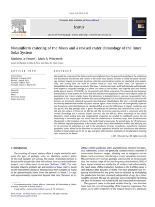
  • 5. M. Le Feuvre, M.A. Wieczorek / Icarus 214 (2011) 1–20 5 sffiffiffiffiffiffiffiffiffiffiffiffiffiffiffiffiffiffiffi v2 from Eqs. (A.51) and (A.54). The impact velocity u is only dependent m s0 ¼ a m 1 þ 2 2 ; ð7Þ on U and C, while the incidence angle h further depends on position. V where am and vm are respectively the lunar semi-major axis and 3.3. Cratering rate velocity. On the cross sectional disk, the distance from the center is denoted by the impact parameter b. Only when b 6 s0 is it possi- To obtain cratering rates from impact rates, we need to convert ble for a hyperbolic orbit to impact the Moon (note that the gravi- the impactor diameters into crater diameters. For this purpose, we tational cross section of the Moon itself is accounted for later in use equations that have been derived in the framework of p-scal- the calculation, see Appendix A.2). The probability distribution of ing dimensional analysis (Holsapple and Schmidt, 1987; Holsapple, encounter conditions p(V) is first calculated according to this new 1993), where the transient crater is given as a function of the pro- definition of the encounter probability. Then, the relative lunar jectile diameter, impact velocity, surface gravity and projectile/tar- encounter velocity U and probability Pm are derived analytically get density ratio (see Appendix A.4). It is assumed that only the for each hyperbolic orbit crossing the Earth–Moon system (Eqs. vertical component of the impact velocity, whose value is obtained (A.19), (A.18), (A.24), (A.25), (A.30)–(A.33)). The probability distri- from the impact angle, contributes to the crater size (Pierazzo bution of lunar encounter conditions, p(U), is then determined by et al., 1997), though other relations could be easily incorporated integrating numerically Pm for all possible hyperbolic orbits of each into this analysis. The scaling equation and parameters are taken encounter V, and for all encounter velocities. Similarly, the impact from the summary of Holsapple and Housen (2007) for the case probability with Earth Pe is determined for each hyperbola, and of porous and non-porous scaling. It will be seen that both forma- the Moon/Earth impact ratio r is calculated over all possible tion regimes are necessary to reconcile the impactor and crater encounters. Mathematically, p(U) and r are given by Eqs. (A.34)– SFDs. We only consider craters that form in the gravity regime, (A.36). where the tensile strength of rock is negligible, that is, craters lar- Note that there is a dependence of the lunar impact rate on the ger than a few hundred meters in competent rock, and larger than Earth–Moon separation distance, am. This distance has evolved out- a few meters in consolidated soils. An increase of the transient cra- ward with time, and we test various separation distances in the ter diameter by wall slumping and rim formation is accounted for simulations. A major difference between our approach and previ- as given in Melosh (1989). Finally, large craters collapse due to ous investigations (Shoemaker and Wolfe, 1982; Zahnle et al., gravity, becoming complex craters, and the relationship between 1998; Zahnle et al., 2001) is that the argument of pericenter of simple and complex crater diameters is taken from Holsapple the hyperbolic orbits is not assumed to precess uniformly within (1993). Putting this altogether, we obtain the relation d(D, u, h) that the Earth–Moon system, but is explicitly given by the encounter gives the impactor diameter d as a function of the crater diameter geometry. Our formulation allows to calculate explicitly lateral D, impact velocity u and incidence angle h (Appendix A.4, Eqs. asymmetries in the lunar cratering rate. (A.63), (A.59)). The impactor diameter d required to create a crater of size D is ultimately a function of k, / and U (see Eqs. (A.51) and 3.2. Impact rate (A.54)). The cratering rate, that is the number of craters larger than D Let us express the cumulative impact flux, that is the number of that form at (k, u) per unit time and area, is objects with diameters greater than d that hit the planet per unit Z time and area, as Cð D; k; uÞ ¼ /ð d; k; /ÞpðUÞdU; ð12Þ U /ð d; k; uÞ ¼ /ð dÞ Â D/ðk; uÞ; ð8Þ where where k and u are respectively the latitude and longitude, /ð dÞ is d ¼ dðD; k; /; UÞ: ð13Þ the spatially averaged impact rate for projectiles larger than d, and D/(k, u) is the relative impact rate as a function of position, normal- For convenience, we separate the cratering rate into ized to the global average. Using our normalized impactor SFD, the average impact rate expresses as Cð D; k; uÞ ¼ Cð DÞ Â DCð D; k; uÞ: ð14Þ /ð dÞ ¼ /ð 1Þsð dÞ; ð9Þ where Cð DÞ is the spatially averaged rate and DC(D, k, u) is the relative spatial variation. Note that DC depends on D, though in and /ðd 1Þ is obtained from the impact ratio between the target practice, this dependence is moderate (see next section). and Earth, r, and the terrestrial impact rate /e ðd 1Þ as /ð 1Þ ¼ r /e ð 1Þ: ð10Þ 4. Results The net spatial asymmetry D/(k, u) is found by integrating the spa- 4.1. Crater size-frequency distributions tial asymmetries d/(k, u, U) associated with each encounter geometry: We first present our synthetic size-frequency distribution of lu- Z nar craters. Following the terminology of Marchi et al. (2009), we D/ðk; uÞ ¼ d/ðk; u; UÞpðUÞdU; ð11Þ refer to this as a model production function. We compare our mod- U el production function with the two standard measured production where d/ is given in Appendix A.3 as a function of the Safronov functions of Neukum (1983, 1994) and Hartmann (Basaltic Volca- parameter C and obliquity of the target (Eqs. (A.47)–(A.49)). The nism Study Project, 1981; Hartmann, 1999). We note that the impact flux is homogeneous for C = 1, that is, for encounter veloc- two are in good agreement over the crater diameter range from ities negligible with respect to the target’s surface gravitational po- 300 m to 100 km, but differ between 2 and 20 km, with a tential (Eq. (3)). On the other hand, for C = 0, encounter trajectories maximum discrepancy of a factor 3 at 5 km. are straight lines, and the impact flux is a simple geometrical pro- Using the traditional non-porous scaling relations and a jection of the spatially uniform encounter flux (on a plane perpen- standard target density of 2800 kg mÀ3, we calculate that dicular to the radiant) onto the target’s spherical surface. The 2.88 Â 10À11 craters larger than 1 km would be created each year associated impact velocities and incidence angles are calculated on the lunar surface by the present impactor population. Using
  • 6. 6 M. Le Feuvre, M.A. Wieczorek / Icarus 214 (2011) 1–20 the time-dependence established by Neukum (1983) that predicts 1 dz ðzÞ ¼ ððT À zÞdp þ zdnp Þ for z 6 T; a quasi-constant impact flux over the last $3 Ga, the Hartmann T ð17Þ and Neukum production functions return respective values of dz ðzÞ ¼ dnp for z P T; 7.0 Â 10À13 and 8.2 Â 10À13, which are about 10 times lower, implying that the present flux must be considerably larger than the time averaged value. with dp and dnp the impactor diameters respectively required from However, by using the porous scaling law instead, in order to the porous and non-porous regimes. In the calculation of dnp, the account for the presence of megaregolith on the lunar surface, target density is set to 2800 kg mÀ3 (solid rocks), whereas we as- our calculated spatially averaged lunar cratering rate is sume in calculating dp that the density of the porous material is À2 2500 kg mÀ3, based on Bondarenko and Shkuratov (1999) who in- C m ðD 1Þ ¼ 7:5 Â 10À13 yrÀ1 km ; ð15Þ ferred an upper regolith density comprised between 2300 and a value in excellent agreement with the two measured production 2600 kg mÀ3 from correlations between the surface regolith thick- functions under the assumption of a constant impact flux over the ness and the Soderblom’s crater parameter (Soderblom and Lebof- last $3 Ga. sky, 1972). We note that given the simplicity of our crater-scaling Let us now reconcile the entire shape of the measured produc- procedure in the transition zone, the correspondance between T tion functions with the observed impactor population. As shown in and the actual megaregolith thickness should not be expected to Fig. 2, the two measured distributions are very well fitted by using be exact. the porous regime for small craters (D 2 km), and the non-porous As shown in Fig. 2, our model reproduces both the Hartmann regime for larger craters (D 20 km). We model a simple smooth and Neukum production functions within the 100 m – 300 km transition between the two regimes by considering that the impac- diameter range, for respective values of T equal to 250 and 700 tor size d required to create a crater of diameter D is a linear com- m, respectively. For these diameter ranges, the maximum discrep- bination of the sizes required from the porous and non-porous ancy between our model and the Neukum production function is scaling relations, the influence of each regime depending on the only 30% at 200 m, and always less than 20% for craters larger than depth of material excavated by the crater. The depth of excavation 500 m. Below 100 m, we note that our model is in reasonable zT is about 1/10 of the transient crater diameter DT, and does not agreement with the Neukum production function, and we leave seem to depend on target properties (Melosh and Ivanov, 1999). the implications for the contribution of secondary craters to fur- The impactor size is averaged over the depth of excavation: ther investigations. The model production function proposed by Z zT Marchi et al. (2009) is also shown in Fig. 2. A detailed comparison 1 with this latter study is given in the discussion section. d¼ dz ðzÞ dz; ð16Þ zT 0 The use of porous scaling was first suggested by Ivanov (2006) where dz is the impactor size required by the material at depth z, (see also Ivanov, 2008; Ivanov et al., 2007), and is a natural conse- given by the porous regime at the surface, by the non-porous re- quence of a highly fractured megaregolith on airless bodies. Also gime at depths larger than a given ‘‘megaregolith thickness’’ T, natural is to expect that the thickness of the megaregolith will de- and by a linear combination between z = 0 and z = T: pend upon both age and local geology. We note that the need for a transition regime falls within the diameter range where the mea- sured production functions differ the most (excluding very large craters). We suspect that this is partially a result of the Hartmann production function being based on crater counts performed solely over mare units, whereas the Neukum production function also in- 10−5 cludes older highlands terrains (Neukum et al., 2001a). Estimated megaregolith thicknesses are roughly consistent with 10−6 seismic models of the lunar crust (e.g., Warren and Trice, 1977; 10−7 Lognonné et al., 2003) that generally predict reduced seismic Cumulative number (km−2 yr − 1) 10−8 velocities for the upper km, which is attributed to an increased 10−9 porosity and fractures. Furthermore, seismic data at the Apollo 17 landing site, overlaid by mare basalt, indicates that the upper 10−10 250 / 400 m show a very low P-wave velocity with respect to the 10−11 deeper basalt (Kovach and Watkins, 1973; Cooper et al., 1974), 10−12 the lower estimate being in agreement with our calculated megar- 10−13 egolith depth of 250 m for the Hartmann production function. Fi- nally, Thompson et al. (1979) show by analysis of radar and 10−14 infrared data (which are dependent on the amount of near surface 10−15 Neukum et al. (2001) rocks) that craters overlying highlands show different signatures 10−16 Hartmann (1999) for craters greater and less than 12 km, and that mare craters down 10−17 Marchi et al. (2009) to 4 km in diameter possess a similar signature to that of highlands Model, megaregolith 700 m craters greater than 12 km. They attribute this difference to the 10−18 Model, megaregolith 250 m presence of a pulverized megaregolith layer that is thicker in the 10−19 older highlands than the younger mare. 0.01 0.1 1 10 100 By the use of a porous regime dictated by the properties of a Crater diameter (km) megaregolith, our model production function reproduces the mea- sured crater distributions in shape and in the absolute number of Fig. 2. Model production function of lunar craters, for 1 yr, in comparison with the craters formed over the past 3 Ga, under the assumption of a con- Hartmann and Neukum measured production functions, and the model production stant impact flux. We caution that our simple formulation of the function of Marchi et al. (2009). Respective megaregolith thicknesses of 700 and 250 m allow to fit either the Neukum or Hartmann production functions in the porous/non-porous transition does not account for the temporal diameter range 2–20 km. The thin dotted red curve is obtained by using only the evolution of the megaregolith and that the inferred megaregolith non-porous scaling relation. thicknesses are only qualitative estimates.
  • 7. M. Le Feuvre, M.A. Wieczorek / Icarus 214 (2011) 1–20 7 The present Earth–Moon distance has been used in the above For illustrative purpose, Rc is shown for the inner planets in Fig. 3 by calculation of the lunar cratering rate, and temporal variations in assuming that craters with diameters less than 10 km form in a por- the lunar semi-major axis could, in principle, modify the Earth/ ous soil on both the planet and Moon, while craters with greater Moon impact ratio and encounter velocity distribution with the sizes form in solid rocks (except for the Earth and Venus where only Moon. Nevertheless, it is found in our simulations that, for a lunar the non-porous regime is used). Note that Rc can be easily calcu- semi-major axis as low as 20 Earth radii, the average lunar crater- lated from Eq. (18) and Table 2 for a different (and more realistic) ing rate is changed by less than 3%. This implies that both the transition between porous and non-porous regimes. shielding and gravitational focusing of projectiles by the Earth The mean impact velocity on the Moon is calculated to be are of very moderate effects, especially since the Moon is believed um ¼ 19:7 km sÀ1 . The full probability distribution of impact veloc- to have spent the vast majority of its history beyond 40 Earth radii. ities for each planet is shown in Fig. 4. The quantities /=/m ; u=um Our globally averaged planetary cratering rates Cð DÞ are fitted by 10th-order polynomials for the Moon and inner planets. The coefficients (with units of yrÀ1 km2) are listed in Table 2. Since 4 the megaregolith thickness is not necessarily the same on each pla- net, and may depend on the age and geology of the surface, coeffi- cients are given for the two scaling regimes (T = 1 and T = 0 km) for diameters between 0.1 and 1000 km (except for the Earth and 3 Venus, where only non-porous scaling is given). A linear transition simpler than ours can be used by defining two threshold diame- ters, Dp and Dnp, such that the porous and non-porous regime ap- Mercury R c (D) plies alone respectively below Dp and above Dnp. The cratering Venus rate in the transition regime is then calculated as Cð DÞ ¼ 2 Earth C ðD ÞÀC ðD Þ C p ð Dp Þ þ np Dnp ÀDpp p ðD À Dp Þ, where Cp and Cnp are given in Ta- Mars np ble 2 in the porous and non-porous columns, respectively. Note that the martian cratering rate is sensitive to the eccentricity of the planet, since the number of potential impactors increases dra- 1 matically as this planets gets closer to the Main Asteroid Belt (Le Feuvre and Wieczorek, 2008; Ivanov, 2001). In addition to calculat- ing the present day martian cratering rate, we also used the prob- ability distribution of the martian eccentricity provided by Laskar (2008) to calculate an average over the past 1 Ga (note that this va- 0 0.1 1 10 100 1000 lue is nearly insensitive for longer averages). Planetary size-frequency distributions are generally expressed D (km) with respect to the lunar one. This is done by defining the size- Fig. 3. Planetary cratering ratios with respect to the Moon, for craters larger than a dependent quantity Rc, which is the cratering ratio with respect given diameter D. For illustrative purposes, craters with D 10 km and D 10 km to the Moon, are respectively assumed to form in the porous and non-porous regimes. Curves are not shown for Venus and the Earth for D 10 km, since the porous regime is not Cð DÞ expected, and erosion or atmospheric shielding are known to be of significant Rc ð DÞ ¼ : ð18Þ C m ð DÞ influence at these sizes. Table 2 P Planetary crater size-frequency distributions for 1 yr (kmÀ2): log Cð DÞ ¼ 10 C i ðlog Dkm Þi ; D 2 ½0:1—1000Š km. i¼0 Moon Moon Mercury Mercury Venus Non-porous Porous Non-porous Porous Non-porous C0 À0.1049E+02 À0.1206E+02 À0.9939E+01 À0.1159E+02 À0.1073E+02 C1 À0.4106E+01 À0.3578E+01 À0.3994E+01 À0.3673E+01 À0.4024E+01 C2 À0.8715E+00 0.9917E+00 À0.1116E+01 0.9002E+00 À0.4503EÀ01 C3 0.1440E+01 0.7884E+00 0.1269E+01 0.9609E+00 0.1374E+01 C4 0.1000E+01 À0.5988E+00 0.1272E+01 À0.5239E+00 0.2433E+00 C5 À0.8733E+00 À0.2805E+00 À0.8276E+00 À0.3622E+00 À0.7040E+00 C6 À0.2725E+00 0.1665E+00 À0.3718E+00 0.1508E+00 À0.3962EÀ01 C7 0.2373E+00 0.3732EÀ01 0.2463E+00 0.5224EÀ01 0.1541E+00 C8 0.9500EÀ02 À0.1880EÀ01 0.2091EÀ01 À0.1843EÀ01 À0.8944EÀ02 C9 À0.2438EÀ01 À0.1529EÀ02 À0.2756EÀ01 À0.2510EÀ02 À0.1289EÀ01 C10 0.3430EÀ02 0.7058EÀ03 0.3659EÀ02 0.8053EÀ03 0.2102EÀ02 Earth Mars (long term) Mars (long term) Mars (today) Mars (today) Non-porous Non-porous Porous Non-porous Porous C0 À0.1099E+02 À0.1089E+02 À0.1213E+02 À0.1082E+02 À0.1207E+02 C1 À0.3996E+01 À0.4068E+01 À0.3124E+01 À0.4072E+01 À0.3134E+01 C2 0.2334E+00 0.2279E+00 0.1295E+01 0.2157E+00 0.1293E+01 C3 0.1333E+01 0.1422E+01 0.1542E+00 0.1426E+01 0.1713E+00 C4 0.2286EÀ02 0.2470EÀ01 À0.7519E+00 0.3330EÀ01 À0.7518E+00 C5 À0.6476E+00 À0.7150E+00 0.3125EÀ01 À0.7171E+00 0.2232EÀ01 C6 0.2875EÀ01 0.2056EÀ01 0.1779E+00 0.1856EÀ01 0.1786E+00 C7 0.1313E+00 0.1535E+00 À0.2311EÀ01 0.1540E+00 À0.2129EÀ01 C8 À0.1410EÀ01 À0.1526EÀ01 À0.1369EÀ01 À0.1510EÀ01 À0.1396EÀ01 C9 À0.1006EÀ01 À0.1252EÀ01 0.2623EÀ02 À0.1255EÀ01 0.2492EÀ02 C10 0.1810EÀ02 0.2247EÀ02 0.5521EÀ05 0.2246EÀ02 0.3212EÀ04
  • 8. 8 M. Le Feuvre, M.A. Wieczorek / Icarus 214 (2011) 1–20 0.20 velocity is added to the projectile velocity for impacts at the apex, whereas it is subtracted at the antapex. The apex/antapex ratio is Mercury 1.37. We note that there is a negligible nearside/farside effect: Venus the nearside experiences the formation of about 0.1% more craters Earth that the farside. The Earth does indeed concentrate very low incli- 0.15 Moon nation (and moderate velocity) projectiles onto the lunar nearside, Mars but these are not numerous enough to influence the global distribution. Probability The lateral cratering variations depend on the crater size since 0.10 the size-frequency distribution of impactors s(d) is not a simple power law, and the impact conditions are not everywhere the same. Nevertheless, the maximum/minimum cratering ratio varies only by about 5% for D ranging from 30 m to 300 km. Consequently, 0.05 for the following discussion, we shall consider that DC(D, k, u) ’ DC(1, k, u). For smaller Earth–Moon distances am, the apex/antapex effect increases as the lunar velocity increases. Between 20 and 60 Earth radii, this dependency is fit by the simple equation 0.00 10 20 30 40 50 60 70 80 90 am CðapexÞ=CðantapexÞ ¼ 1:12eÀ0:0529 Re þ 1:32; ð19Þ Impact velocity (km/s) where Re is the Earth radius. Over this range of Earth–Moon separa- Fig. 4. Probability distribution of impact velocities for the Moon and terrestrial tions, latitudinal variations and the nearside/farside effect are found planets. to vary by less than 1%. These calculations assume that the lunar and g/gm, that give the relative impact flux, impact velocity and obliquity stayed equal to its present value in the past. surface gravity with respect to the Moon, are given in Table 3 for Fig. 6 plots the relative cratering rate DC as a function of the the inner planets. Mars experiences a high impact rate with respect angular distance from the apex of motion for the present Earth– to the Moon (about 3) due to its proximity to the main asteroid Moon distance, and compares this with the counts of rayed craters belt. In comparison, the martian cratering ratio is reduced (be- with diameters greater than 5 km given in Morota et al. (2005). tween about 0.5 and 2.5) because the impact velocity on Mars is Rayed craters are younger than about 1 Ga (Wilhelms et al., significantly lower than on the Moon, requiring larger (and hence 1987), which should corresponds to an Earth–Moon separation dis- less numerous) impactors to create a crater of a given size. Mercury tance very close to the present one (Sonett and Chan, 1998; Eriks- exhibits also a high impact rate, and the impact velocity is about son and Simpson, 2000). As is seen, the model compares favorably twice as large as on the Moon, resulting in a high value of the cra- to the data. tering ratio Rc, comprised between 2 and 4. The impact rate is lar- We note that the impact rate exhibits nearly the same behavior ger on the Earth and Venus than on the Moon, as these planets as the cratering rate, but with a reduced amplitude. The pole/equa- possess a higher gravitational attraction. Their higher surface grav- tor ratio is 0.90, whereas the apex/antapex ratio is 1.29. The latitu- ities compensate the differences in impact velocities with the dinal cratering variations are enhanced with respect to the impact Moon, and Rc is comprised between 0.5 and 1.5 for the Earth and rate variations, as the mean impact angle and impact velocity are between 1 and 2 for Venus. smaller at the poles than at the equator (respectively by 2.5° and 500 m/s), requiring a larger projectile to create the same crater size. As large projectiles are less numerous than small ones, the im- 4.2. Spatial variations pact rate at the poles is smaller than the cratering rate (Le Feuvre and Wieczorek, 2008). This is also true for the apex/antapex asym- The relative spatial cratering variations on the Moon, metry, as the average impact velocity is 500 m/s higher at the apex DC(D, k, u), are shown in Fig. 5 for the present Earth–Moon dis- than at the antapex. However, the increase is moderate, as the tance of about 60 Earth radii, and for crater diameters larger than mean impact angle is only about 1.5° smaller. 1 km. The cratering rate varies from approximately À20% to +25% It is seen in Fig. 7 that our predicted apex/antapex effect differs with respect to the global average. It is minimized at about from that of Zahnle et al. (2001). These authors describe their vari- (±65°N, 90°E), whereas the maximum, which is a factor 1.5 higher, ations of the impact rate as a function of c, the angular distance to is located at the apex of motion (0°N, 90°W). the apex, as Two effects conjugate to give such a distribution. First, a latitu- 0 12 dinal effect, detailed in Le Feuvre and Wieczorek (2008), comes B vm C from the higher proportion of low inclination asteroids associated D/ðcÞ ¼ @1 þ qffiffiffiffiffiffiffiffiffiffiffiffiffiffiffiffiffiffiffiffiffi cos cA ; ð20Þ with the higher probabilities of low inclination encounters. The 2v 2 þ V 2 m pole/equator ratio is 0.80. Second, a longitudinal apex/antapex ef- fect comes from the synchronous rotation of the Moon and the where V ’ 19 km sÀ1 is the mean encounter velocity with the higher relative encounter velocities at the apex. The lunar orbital Earth–Moon system. We are able to reproduce their analytical solu- Table 3 Impact rate, mean impact velocity and surface gravity for the inner planets, normalized to the Moon’s. Moon Mercury Venus Earth Mars (long term) Mars (today) Impact rate ratio 1 1.82 1.75 1.58 2.76 3.20 Mean velocity ratio 1 2.16 1.28 1.04 0.53 0.54 Surface gravity ratio 1 2.2 5.3 5.9 2.2 2.2
  • 9. M. Le Feuvre, M.A. Wieczorek / Icarus 214 (2011) 1–20 9 90° 60° 30° 180° 210° 240° 270° 300° 330° 0° 30° 60° 90° 120° 150° 180° −30° −60° −90° 0.85 0.90 0.95 1.00 1.05 1.10 1.15 1.20 1.25 Relative cratering rate Fig. 5. Relative cratering rate on the Moon for the current Earth–Moon distance and for crater diameters larger than 1 km. This image is plotted in a Mollweide projection centered on the sub-Earth point. 1.2 1.4 1.1 Relative impact rate Relative cratering rate 1.2 1 1.0 0.8 0.9 0.6 0 30 60 90 120 150 180 0 30 60 90 120 150 180 Angular distance from apex (º) Angular distance to apex (°) Fig. 6. Relative lunar cratering rate as a function of angular distance from the apex of motion. Rayed crater data are for crater diameters greater than 5 km from Morota Fig. 7. Relative lunar impact rate as a function of the angular distance from the et al. (2005) that were counted between approximately [70°E, 290°E] in longitude apex (solid black), in comparison with the equation from Zahnle et al. (2001) (solid and [À42°N, 42°N] in latitude. In comparison, the predicted apex/antapex cratering gray). The latter is reproduced if the model forces latitudinal isotropy of encounter effect is shown over the same count area (solid black) and for the entire Moon inclinations (dotted black). (dotted black). 2008). Spatial variations in the impact flux and cratering rate are parameterized by a sum a spherical harmonic functions tion, but only under the condition where we force the encounter inclinations with respect to the lunar orbit plane to be isotropic in X X 1 l space. These authors used Öpik equations (Shoemaker and Wolfe, DCðk; uÞ ¼ C lm Y lm ðk; uÞ; ð21Þ l¼0 m¼Àl 1982) for hyperbolic orbits that were assumed to precess uniformly inside the planet–Moon system. We nevertheless point out that where Ylm is the spherical harmonic function of degree l and order Zahnle et al. (2001) applied Eq. (20) to the moons of Jupiter, where m, Clm is the corresponding expansion coefficient, and (k, u) repre- this approximation might be valid. sents position on the sphere in terms of latitude k and longitude We next provide analytical solutions for the relative variations u, respectively. The real spherical harmonics are defined as of both the impact and cratering rates on the Moon. We also give ( solutions for the latitudinal variations presented on the terrestrial Plm ðsin kÞ cos mu if m P 0 Y lm ðk; uÞ ¼ ð22Þ planets in Le Feuvre and Wieczorek (2008). Two values are quoted Pljmj ðsin kÞ sin jmju if m 0; for Mars, one that corresponds to its present obliquity and eccen- tricity and the other to averaged results using variations over and the corresponding unnormalized Legendre functions are listed 3 Ga as given in Laskar et al. (2004) (see Le Feuvre and Wieczorek, in Table 4. Many of the expansion coefficients are nearly zero since
  • 10. 10 M. Le Feuvre, M.A. Wieczorek / Icarus 214 (2011) 1–20 Table 4 the following relationship between the number of craters with Unnormalized associated Legendre functions. diameters greater than 1 km and the age of the geologic unit: l, m Plm(sin k) NðD 1; tÞ ¼ aðebt À 1Þ þ ct; ð23Þ 0, 0 1 1, 1 cosk where NðD 1; tÞ is given per 106 km2, t is the age expressed in Ga, 2, 0 1 2 2 ð3 sin k À 1Þ and a = 5.44 Â 10À14, b = 6.93 and c = 8.38 Â 10À4. This relationship 2 2, 2 3 cos k 3, 1 3 2 is essentially linear over the last 3.3 Ga (constant cratering rate in 2 ð5 sin k À 1Þ cos k 4, 0 1 4 2 time) and approximately exponential beyond. The data used to con- 8 ð35 sin k À 30 sin k þ 3Þ struct this empirical curve are obtained from radiometric ages of the Apollo and Luna rock samples, compared to the crater density covering the associated geologic unit. We emphasize that no agreed Table 5 upon calibration data exist between 1 and 3 Ga and beyond 3.9 Ga Spherical harmonic coefficients of the lunar relative impact flux D/(k, u) for Earth– Moon separations of 30, 45, and 60 Earth radii. (Stöffler and Ryder, 2001). We also note that Eq. (23) was originally obtained using age estimates of the highland crust and Nectaris im- Clm 30 Earth radii 45 Earth radii 60 Earth radii pact basin, both of which are disputed and considerably older than C0,0 1 1 1 3.9 Ga. C1,À1 À1.7779020 Â 10À1 À1.4591830 Â 10À1 À1.2670400 Â 10À1 Accounting for our calculated spatial variations, we first convert C2,0 À6.3209891 Â 10À2 À6.2923420 Â 10À2 À6.2755592 Â 10À2 the measured crater density at a given site, N(D 1, k, u), into the C2,2 À1.7937283 Â 10À3 À1.2524090 Â 10À3 À9.8998262 Â 10À4 C4,0 À9.9735381 Â 10À3 À1.0141450 Â 10À2 À1.0222370 Â 10À2 corresponding spatially averaged quantity: NðD 1Þ ¼ NðD 1; k; uÞ=DCðD 1; k; uÞ: ð24Þ Table 6 The cratering asymmetry DC is given in Table 2, and we use the Spherical harmonic coefficients of the lunar relative cratering rate DC(D 1,k, u) for function that corresponds to the present Earth–Moon separation Earth–Moon separations of 30, 45, and 60 Earth radii. for cratered surfaces that are less than 1 Ga (consistent with the ti- Clm 30 Earth radii 45 Earth radii 60 Earth radii dal deposit data of Sonett and Chan (1998)). We choose a Earth– C0,0 1 1 1 Moon separation of 40 Earth radii for units that are older than C1,À1 À2.2715950 Â 10À1 À1.8571530 Â 10À1 À1.6092760 Â 10À1 3 Ga (based on the tidal deposits data of Eriksson and Simpson C2,0 À1.3954110 Â 10À1 À1.3874170 Â 10À1 À1.3831914 Â 10À1 (2000)). This lunar semi-major axis value corresponds to a lunar C2,2 À3.3499412 Â 10À3 À2.2729362 Â 10À3 À1.7822560 Â 10À3 orbital velocity twice as large as the present one. We further as- C3,À1 2.9040180 Â 10À3 2.3263713 Â 10À3 1.9948010 Â 10À3 C4,0 2.7412530 Â 10À3 2.7863080 Â 10À3 2.8083000 Â 10À3 sume that the lunar obliquity was equal to its present value (nearly zero) for the entire time between 3.9 Ga and the present. The data used to calibrate the crater density versus age relation- ship are listed in Table 9, along with their corrections accounting Table 7 for spatial variations in the cratering rate. We use the crater den- Spherical harmonic coefficients of the relative impact flux D/(k) for the terrestrial planets. sity and ages values quoted in Stöffler and Ryder (2001). We did not attempt to fit crater distributions with our model production Planet C00 C20 C40 function to re-estimate N(D 1) values, since our model already Mercury 1 3.7395410 Â 10À2 À7.9170623 Â 10À3 reproduces very well the Neukum production function that was Venus 1 7.3546990 Â 10À3 À6.0267052 Â 10À3 used to estimate this quantity. For the case of very young calibra- Earth 1 À2.6165971 Â 10À2 À1.8682412 Â 10À3 tion surfaces, we suspect that a thinner megaregolith might change Mars (today) 1 1.6254980 Â 10À1 À1.0738801 Â 10À2 Mars (long-term average) 1 8.7425552 Â 10À2 4.7442493 Â 10À3 the crater distribution with respect to the Neukum production function at sizes larger than one kilometer, but, for small exposure times, the largest observed craters are below this diameter value. Based on the data and interpretations of Norman (2009), we ex- Table 8 clude the Nectaris basin from consideration, as it is possible that Spherical harmonic coefficients of the relative cratering rate DC(D 1, k) for the samples assigned to this basin have instead an Imbrium prove- terrestrial planets. nance. We thus assume that the Descartes formation is not Necta- Planet C00 C20 C40 ris ejecta, but rather Imbrium ejecta with an age of 3.85 Ga. We Mercury 1 4.5850560 Â 10À2 2.4749320 Â 10À3 also exclude the Crisium basin from the fit, due to the uncertain Venus 1 À1.8545722 Â 10À3 3.5865970 Â 10À4 provenance of samples dated at the Luna 20 site. Finally, we use Earth 1 À7.6586370 Â 10À2 2.4353234 Â 10À4 the recent crater counts performed on Copernicus deposits by Mars (today) 1 3.3900970 Â 10À1 2.2655340 Â 10À3 Mars (long-term average) 1 1.7986312 Â 10À1 À4.3484250 Â 10À4 Hiesinger et al. (2010) with high-resolution Lunar Reconnaissance Orbiter images, which agree with a constant impact flux during the last 800 Ma, in contrast to previous studies. the cratering rate is symmetric about both the equator and the axis As seen in Table 9, the spatial correction is in general moderate, connecting the apex and antapex of motion. Only the most signifi- since the calibration terrains are located in the central portion of cant coefficients are listed in Tables 5 and 6, which for most cases the nearside hemisphere, far from the extrema of the spatially- reproduce the data to better than 0.2%. The coefficients for the lat- dependent cratering rate. Nevertheless, we point out that after cor- itudinal variations on the terrestrial planets are listed in Tables 7 rection, the Apennines, Fra Mauro and Descartes formations, which and 8. are all Imbrian in age, exhibit nearly the same globally averaged crater density, which is consistent with our assignment of an 5. Crater chronology Imbrium origin to the Descartes formation, as recently suggested by Norman (2009) (see also Haskin et al., 1998). Neukum et al. (2001a) (see also Neukum, 1983; Strom and We perform a new fit of the calibration point, using the same Neukum, 1988; Neukum and Ivanov, 1994) established empirically functional form as in Eq. (23). Our resulting best parameters are