SlideShare una empresa de Scribd logo
1 de 42
Descargar para leer sin conexión
Gripping IFRS                                                                 Inventories


                                         Chapter 4
                                         Inventories
Reference: IAS 2

Contents:                                                                          Page
   1. Introduction                                                                  137

   2. Definitions                                                                   137

   3. Different classes of inventories                                              137

   4. Recording inventory movement: periodic versus perpetual                       138
      4.1 Overview                                                                  138
          Example 1: perpetual versus periodic system                               138
      4.2 Stock counts, inventory balances and stock theft                          139
          4.2.1 The perpetual system and the use of stock counts                    139
          4.2.2 The periodic system and the use of stock counts                     139
          Example 2: perpetual versus periodic system and stock theft               140
      4.3 Gross profit and the trading account                                      141
          Example 3: perpetual and periodic system: stock theft and profits         142

   5. Measurement: cost                                                             144
      5.1 Overview                                                                  144
      5.2 Cost of purchase                                                          144
          5.2.1 Transport costs                                                     144
                5.2.1.1 Transport/ carriage inwards                                 145
                5.2.1.2 Transport/ carriage outwards                                145
                Example 4: transport costs                                          145
          5.2.2 Transaction taxes                                                   146
                Example 5: transaction taxes                                        146
          5.2.3 Rebates                                                             147
                Example 6: rebates                                                  147
          5.2.4 Discount received                                                   148
                Example 7: discounts                                                148
          5.2.5 Finance costs due to extended settlement terms                      149
                Example 8: extended settlement terms                                149
          5.2.6 Imported inventory                                                  151
                Example 9: exchange rates – a basic understanding                   151
                Example 10: foreign exchange                                        152
      5.3 Cost of conversion                                                        153
          5.3.1 Variable manufacturing costs                                        153
                Example 11: variable manufacturing costs                            153
          5.3.2 Fixed manufacturing costs                                           154
                5.3.2.1 Under-production and under-absorption                       154
                Example 12: fixed manufacturing costs – under-absorption            154
                5.3.2.2 Over-production and over-absorption                         156
                Example 13: fixed manufacturing costs – over-absorption             156
                5.3.2.3 Budgeted versus actual overheads summarised                 157
                Example 14: fixed manufacturing costs – over-absorption             158
                Example 15: fixed manufacturing costs – under-absorption            159


                                             135                               Chapter 4
Gripping IFRS                                                                   Inventories


Contents continued …                                                                   Page

   6. Measurement: cost formulas (inventory movements)                                 160
      6.1 Overview                                                                     160
      6.2 First-in-first-out method (FIFOM)                                            161
          Example 16: FIFOM purchases                                                  161
          Example 17: FIFOM sales                                                      161
          Example 18: FIFOM sales                                                      162
      6.3 Weighted average method (WAM)                                                162
          Example 19: WAM purchases                                                    162
          Example 20: WAM sales                                                        163
      6.4 Specific identification method (SIM)                                         163
          Example 21: SIM purchases and sales                                          163

   7. Measurement of inventories at year-end                                           164
      7.1 Overview                                                                     164
          Example 22: lower of cost or net realisable value                            164
          Example 23: lower of cost or net realisable value                            165
          Example 24: lower of cost or net realisable value                            166
      7.2 Testing for possible write-downs: practical applications                     167
          Example 25: lower of cost or net realisable value – with disclosure          168

   8. Disclosure                                                                       171
      8.1 Accounting policies                                                          171
      8.2 Statement of financial position and supporting notes                         171
      8.3 Statement of comprehensive income and supporting notes                       171
          Example 26: disclosure of cost of sales and depreciation                     171
      8.4 Sample disclosure involving inventories                                      172
          8.4.1 Sample statement of financial position and related notes               172
          8.4.2 Sample statement of comprehensive income and related notes             172
                 8.4.2.1 Costs analysed by nature in the statement of comprehensive
                         income                                                        172
                 8.4.2.2 Costs analysed by function in the statement of
                         comprehensive income                                          173
                 8.4.2.3 Costs analysed by function in the notes to the statement of
                         comprehensive income                                          173

   9. Summary                                                                          175


                                           136                                   Chapter 4
Gripping IFRS                                                                         Inventories


1. Introduction

The topic of inventories is an important area for most companies and thus an important
section to properly understand.

The issues regarding inventories include:
• when to recognise the acquisition of inventory,
• how to measure the initial recognition,
• how to measure inventory subsequently (year-ends and when sold),
• derecognition of inventory when it is sold or scrapped,
• disclosure of inventories in the financial statements.

2. Definitions

Inventories are assets that are (IAS 2.6):
• held for sale in the ordinary course of business; or
• in the process of production for such sale; or
• in the form of materials or supplies to be consumed in the production process or in the
    rendering of services.

Net realisable value is (IAS 2.6):
• the estimated selling price in the ordinary course of business;
• less the estimated costs of completion; and
• less the estimated costs necessary to make the sale.

Fair value is (IAS 2.6):
• the amount for which an asset could be exchanged, or a liability settled,
• between knowledgeable, willing parties in an arm’s length transaction.

The difference between a fair value and a net realisable value is essentially as follows:
• a fair value is what is referred to as an non-entity-specific value, since it is determined by
   market forces; whereas
• a net realisable value is what is referred to as an entity-specific value because it is affected
   by how the entity plans to sell the asset.

3. Different classes of inventories

The type or types of inventories that an entity may have depends largely on the type of
business: retail, manufacturer and service providers, being the most common types.

If the entity runs a retail business, then the inventory will generally be called: merchandise.
A manufacturing business will generally call his inventory:
• finished goods;
• work-in-progress; and
• raw materials.

Another type of inventory held by many types of businesses (e.g. retail, manufacturer and
service provider) includes fuel, cleaning materials and other incidentals, often referred to as:
• consumable stores.

A business may, of course, have any combination of the above types of inventory.


                                               137                                     Chapter 4
Gripping IFRS                                                                          Inventories


4. Recording inventory movements: periodic versus perpetual

4.1 Overview

Inventory movements may be recognised using either the perpetual or periodic system.

The perpetual system refers to the constant updating of both the inventory and cost of sales
accounts for each purchase and sale of inventory. The balancing figure will represent the
value of inventory on hand at the end of the period. This balance is checked by performing a
stock count at the end of the period (normally at year-end).

The periodic system simply accumulates the total cost of the purchases of inventory in one
account, (the purchases account), and updates the inventory account on a periodic basis (often
once a year) through the use of a physical stock count. The balancing figure, in this case, is
the cost of sales.

Example 1: perpetual versus periodic system
                                                            C
 Opening inventory balance                                 55 000
 Purchases during the year (cash)                         100 000

 A stock count at year-end reflected 18 000 units on hand (cost per unit: C5).

 Required:
 Show the t-accounts using
 A. the perpetual system assuming that 13 000 units were sold during the year; and
 B. the periodic system.

Solution to example 1A: using the perpetual system

              Inventory (Asset)                                Cost of Sales (Expense)
O/ balance    55 000 Cost of sales (2) 65 000         Inventory (2) 65
                                                      000
Bank (1)     100 000    C/ balance c/f 90 000
             155 000                  155 000
C/ balance (3) 90 000
(1) The cost of the purchases is debited directly to the inventory (asset) account.
(2) The cost of the sale is calculated: 13 000 x C5 = C65 000 (since the cost per unit was
    constant at C5 throughout the year, the cost of sales would have been the same
    irrespective of whether the FIFO, WA or SI method was used).
(3) The final inventory on hand at year-end is calculated as the balancing figure by taking the
    opening balance plus the increase in inventory (i.e. purchases) less the decrease in
    inventory (i.e. the cost of the sales): 55 000 + 100 000 – 65 000 = 90 000. This is then
    compared to the physical stock count that reflected that the balance should be 90 000. No
    adjustment was therefore necessary.

Solution to example 1B using the periodic system

                 Purchases                                           Trading Account
Bank (2)     100 000 T/ account(5) 000                   Inventory o/b(3) 55    Inventory c/b(4) 90
                                                                        000                     000
                                                          Purchases (5) 000       Total c/f (6) 65
                                                                                                000
                                                                    155 000                 155 000
                                                      Total b/f (6) 65 000

                                                138                                      Chapter 4
Gripping IFRS                                                                        Inventories


              Inventory (Asset)
O/ balance(1) 55 000 T/ account(3) 000
T/ account(4) 90 000

This balance will remain as C55 000 for the entire period until such time as the stock count is
performed.
(1) The purchases are recorded in the purchases account during the period (this account will
    be closed off at the end of the period to the trading account).
(2) The closing balance of the inventory account is determined at the end of the period by
    physically counting the inventory on hand and valuing it (C90 000). In order for the
    closing balance to be recorded, the opening balance of C55 000 needs to first be removed
    from the asset account by transferring it to the trading account.
(3) The inventory is counted and valued via a physical stock count (which is typically
    performed on the last day of the period, being the end of the reporting period). This
    figure is debited to the inventory account with the credit-entry posted to the trading
    account: given as C90 000
(4) The total of the purchases during the period is transferred to the trading account.
(5) Notice how the trading account effectively records the cost of sales and that the cost of
    sales is the same as if the perpetual system had been used instead: 65 000. Incidentally,
    the inventory balance is also the same, irrespective of the method used: 90 000.

4.2 Stock counts, inventory balances and stock theft

In example 1, the cost of sales and inventory balances are not affected by whether the periodic
or perpetual system is used (i.e. cost of sales was C65 000 and inventory was C90 000 in part
A and part B). This may not always be the case however, since a disadvantage of the periodic
system is that any stock thefts will remain undetected. The periodic system is, however, still
useful to small businesses due to its practical simplicity.

4.2.1 The perpetual system and the use of stock counts

When using the perpetual system, the accountant is able to calculate the balance on the
inventory account without the use of a stock count. This balance, however, reflects what the
balance should be – not necessarily what the actual balance is. A sad truth of our society is
that it is plagued by theft. Therefore, even though the accountant is not reliant on the stock
count, a stock count is performed as a control measure. In other words, the balance calculated
by the accountant is checked by performing a stock count at the end of the period (normally at
year-end).

If the physical count reveals a lower stock level than is reflected by the balance on the
inventory account, the difference will be accounted for as a stock theft (expense) (if the
physical count reflects more stock than appears in the inventory account, then this suggests
that an error may have occurred in recording the purchases or sales during the period).

4.2.2 The periodic system and the use of stock counts

When using the periodic system, the accountant does not have any idea of what his cost of
sales are until the stock count is performed. Since we are using the stock count to calculate
the cost of sales, the accountant will also not have an idea of what the inventory balance
should be (if we had the cost of sales figure, we could have calculated the closing balance as:
opening balance + purchases – cost of sales). In short: when using the periodic system, the
accountant is unable to calculate the balance on the inventory account without the use of a
stock count. If the accountant does not know what the balance should be, the stock count will
not be able to highlight any stock thefts.


                                              139                                     Chapter 4
Gripping IFRS                                                                         Inventories


The fact that any stock thefts will remain undetected if the periodic system is used is shown in
this next example.

Example 2: perpetual versus periodic system and stock theft
                                               C                      Units
 Opening inventory balance                        55 000               11 000
 Purchases during the year (cash)                100 000               20 000

 A stock count at year-end reflected 16 000 units on hand (cost per unit: C5).

 Required:
 Show the t-accounts using
 A. the perpetual system assuming that the company sold 13 000 units during the year; and
 B. the periodic system.

Solution to example 2A using the perpetual system and stock theft

               Inventory (Asset)                                Cost of sales (Expense)
O/ balance          55 Cost of S      65 000         Inventory (2) 65
                  000 (2)                            000
Bank (1)           100 Subtotal       90 000
                   000 c/f
                  155                    155
                  000                    000
Subtotal (3)        90 Cost of        10 000
                  000 T(4)
                        C/ bal c/f    80 000
                    90                90 000
                  000
C/                  80
balance(5)        000

                                                                Cost of theft (Expense)
                                                     Inventory (4) 10
                                                     000


(1) The cost of the purchases is debited directly to the inventory (asset) account.
(2) The cost of the sale is calculated: 13 000 x C5 = C65 000 (since the cost per unit was
    constant at C5 throughout the year, the cost of sales would have been the same
    irrespective of whether the FIFO, WA or SI method was used). If the business has very
    few sales or has a sophisticated system, the inventory and cost of sales accounts are
    updated immediately for each sale that takes place. This example processes the
    cumulative sales for the year.
(3) The final amount of inventory that should be on hand at year-end is calculated as the
    balancing figure by taking the opening balance plus the increase in inventory (i.e.
    purchases) less the decrease in inventory (i.e. the cost of the sales): 55 000 + 100 000 – 65
    000 = 90 000
(4) A stock count is performed and whereas there should have been 18 000 units on hand at
    year-end (11 000 + 20 000 – 13 000 units), there are only 16 000 units. It is therefore
    clear that 2 000 units have been stolen. The cost of this theft is therefore 10 000 (2 000 x
    C5).
(5) The closing balance of inventory must reflect the reality and therefore the balance has
    been reduced from what it should have been (90 000) to what it is (80 000).


                                               140                                        Chapter 4
Gripping IFRS                                                                          Inventories


Solution to example 2B using the periodic system and stock theft

                 Purchases                                         Trading Account
Bank (2)     100 000 T/account(5) 100 000                Inventory o/b(3) 55 Inventory c/b    (4)
                                                                                               80
                                                                        000                   000
                                                          Purchases (5) 000  Total c/f (6)     75
                                                                                              000
                                                                     155 000              155 000
                                                     Total b/f (6)    75 000


              Inventory (Asset)
O/ balance(1) 55 000 Trade a/c(3)     000
Trade a/c(4) 80 000

(1) This balance will remain as C55 000 for the entire period until such time as the stock
    count is performed.
(2) The purchases are recorded in the purchases account during the year (this account will be
    closed off at the end of the period to the trading account).
(3) The closing balance of the inventory account is determined at the end of the period by
    physically counting the inventory on hand and valuing it (C90 000). In order for the
    closing balance to be recorded, the opening balance of C55 000 needs to first be removed
    from the asset account by transferring it to the trading account.
(4) The inventory is counted and valued via a physical stock count (which is typically
    performed at the end of the reporting period). This figure is debited to the inventory
    account with the credit-entry posted to the trading account: C80 000 (16 000 x C5).
(5) The total of the purchases during the period is transferred to the trading account.
(6) The trading account effectively records the cost of sales. Whereas the perpetual system in
    Part A indicated that cost of sales was 65 000 and that there was a cost of theft of 10 000,
    this periodic system indicates that cost of sales is 75 000. In other words, the periodic
    system assumed that all missing stock was sold. It is therefore less precise in describing
    its expense but it should be noted that the total expense is the same under both systems
    (periodic: 75 000 and perpetual: 65 000 + 10 000). Incidentally, the inventory balance is
    the same under both methods: 80 000.

4.3 Gross profit and the trading account

If one uses the periodic system, the trading account is first used to calculate cost of sales. The
sales account is then also closed off to the trading account, at which point the total on the
trading account (sales – cost of sales) equals the gross profit (or gross loss). This total is then
transferred to (closed off to) the profit and loss account together with all other income and
expense accounts. The total on the profit and loss account will therefore equal the final profit
or loss for the year.

If the perpetual system is used, the trading account is only used to calculate gross profit: it is
not used to calculate cost of sales. The cost of sales account and sales account are transferred
to (closed off to) the trading account. The total on this trading account (sales – cost of sales)
represents the gross profit. This total will be transferred to (closed off to) the profit and loss
account together with all other income and expense accounts. The total on the profit and loss
account will therefore equal the final profit or loss for the year.

The gross profit calculated according to the perpetual system may differ from that calculated
under the periodic system if, for example, stock theft went undetected. The final profit or loss
calculated in the profit and loss account will, however, be the same.

                                               141                                      Chapter 4
Gripping IFRS                                                                           Inventories


The use of the trading account to calculate gross profit and how gross profits can differ is
shown in this next example.

Example 3: perpetual and periodic system: stock theft and profits
                                                    C              Units
 Opening inventory balance                             55 000        11 000
 Purchases during the year (cash)                     100 000        20 000
 A stock count at year-end reflected 16 000 units on hand (cost per unit: C5).
 Revenue from sales totalled C95 000 for the period (cash).

 Required:
 Show the ledger accounts and extracts of the statement of comprehensive income using:
 A. the perpetual system assuming that the company sold 13 000 units during the year; and
 B. the periodic system assuming that sales totalled C95 000.

Solution to example 3A: perpetual system: stock theft and profits

              Inventory (Asset)                                   Cost of sales (Expense)
O/ balance     55 000 Cost of S        65 000         Inventory      65 000 TA (1)             65 000
Bank             100 Subtotal          90 000
                 000 c/f
                 155                     155
                 000                     000
Subtotal       90 000 Cost of T        10 000
b/f
                         C/ bal c/f    80 000
                90 000                 90 000
C/ balance      80 000


                                                                  Cost of theft (Expense)
                                                      Inventory      10 000 P&L (3)            10 000


                                                                     Sales (Income)
                                                      Trade Acc      95 000 Bank              95 000
                                                      (1)


   Trading account (Closing account)                   Profit and loss account (Closing account)
CoS (1)         65 Sales (1)          95              Cost: theft (3) 10 000 Trade A/c     30 000
               000                   000                                     (GP) (2)
P&L (2)         30                                    Total c/f       20 000
               000
                95                    95                             30 000                   30 000
               000                   000
                                                                              Total   b/f     20 000
                                                                              (4)

(1) Sales and cost of sales are transferred to the trading account.
(2) The total on the trading account (gross profit) is transferred to the profit and loss account.
(3) All other income and expenses are closed off at the end of the year to the profit and loss
    account.


                                                142                                         Chapter 4
Gripping IFRS                                                                          Inventories


(4) If there were no other income and expense items, then this total represents the final profit
    for the year. It would then be transferred to the equity account: retained earnings.

Company name
Statement of comprehensive income
For the period ended …. (extracts)
                                                                          CY              PY
                                                                           C               C
Revenue from sales                                                        95 000           x
Cost of sales                                                            (65 000)         (x)
Gross profit                                                              30 000           x
Cost of theft                                                            (10 000)         (x)
Profit before considering other income and                                20 000           x
expenses

Solution to example 3B: periodic system: stock theft and profits

             Inventory (Asset)                                      Sales (Income)
O/            55 000 TA               55 000           TA (2)       95 000 Bank            95 000
balance
TA            80 000


                 Purchases
Bank             100 TA             100 000
                 000


    Trading account (Closing account)                   Profit and loss account (Closing account)
Inv o/bal    55 000 Inv c/bal     80 000                                     TA (GP) (3)        20
                                                                                               000
Purchases        100 Total c/f       75 000
                 000
                 155                155 000
                 000
Total b/f     75 000 Sales (2)       95 000
(1)

P&L (3)       20 000
              95 000                 95 000


(1) The total brought forward on the trading account represents the cost of inventory
    (assumed to be cost of sales).
(2) Sales are credited to the trading account.
(3) The balance on the trading account represents the gross profit and this is transferred to the
    profit and loss account. All other income and expense accounts are then also transferred
    to (closed off to) the profit and loss account. The profit and loss account therefore
    converts gross profit into the final profit for the period.


Company name
Statement of comprehensive income
For the period ended …. (extracts)
                                                                          CY              PY


                                                 143                                    Chapter 4
Gripping IFRS                                                                         Inventories


                                                                         C                 C
Revenue from sales                                                        95 000           x
Cost of sales                                                            (75 000)         (x)
Gross profit (4)                                                          20 000           x

(4) Notice how the gross profit in the statement of comprehensive income is 20 000 under the
    periodic system but is 30 000 under the perpetual system. The final profit in both cases
    is, however, 20 000.

5. Measurement: cost (IAS 2.10)

5.1 Overview

The costs that one should include in (i.e. capitalise to) inventory include the (IAS 2.10):
• costs to purchase the inventory,
• costs to convert the inventory into a saleable or consumable condition; and
• other costs to bring the inventory to its present location and condition.

5.2 Cost of purchase (IAS 2.11)
The cost of inventory would include all costs directly associated with the acquisition, such as:
• purchase price,
• transport costs (inwards),
• import duties and transaction taxes that are not reclaimable * by the business, and
• other direct costs.
The following costs would be excluded from the cost of inventory:
• import duties and transaction taxes that are reclaimable * by the business,
• financing costs due to extended payment terms.
*: The acquisition of inventory very often involves the payment of transaction taxes and
import duties. Sometimes these taxes or import duties (which are either paid over to the
supplier or directly to the tax authority) and are able to be reclaimed at a later date from the
tax authorities. If they can be reclaimed (recovered), then there is no net cost to the business.
A typical example is the transaction tax levied by many countries: VAT. See chapter 3 for
more information in this regard.
The following would be set-off against the cost of inventory:
• rebates received,
• trade, bulk and cash discounts received,
• settlement discounts received or expected to be received.
Only those costs that are incurred in bringing the inventory to its present location and
condition may be capitalised. The following costs should therefore always be expensed:
• abnormal amounts of wastage;
• storage costs (unless these are directly attributable to the production process, e.g. the cost
   of storage in-between processes that is considered to be unavoidable and normal); and
• selling costs.
5.2.1 Transport Costs
There are two types of transport costs (carriage costs): transport inwards and transport
outwards, each of which being accounted for differently.
5.2.1.1 Transport/ carriage inwards
The cost of transport inwards refers to the cost of transporting the purchased inventory from
the supplier to the purchaser’s business premises. It is a cost that was incurred in ‘bringing the
inventory to its present location’ and should therefore be included in the cost of inventory.

                                               144                                     Chapter 4
Gripping IFRS                                                                        Inventories


5.2.1.2 Transport/ carriage outwards
Frequently, when a business sells its inventory, it offers to deliver the goods to the customer’s
premises. The cost of this delivery is referred to as ‘transport outwards’. It is a cost that is
incurred in order to complete the sale of the inventory rather than to purchase it and may
therefore not be capitalised (since it is not a cost that was incurred in ‘bringing the inventory
to its present location’). Transport outwards should, therefore, be recorded as a selling
expense in the statement of comprehensive income instead of capitalising it to the cost of the
inventory.
Example 4: transport costs
A company purchases inventory for C100 from a supplier. No VAT was charged. The
following additional information is provided:
             Cost of transport inwards                                    C25
             Cost of transport outwards                                   C15
All amounts were on credit and all amounts owing were later paid in cash.
Required:
Calculate the cost of the inventory and show all related journal entries.
Solution to example 4: transport costs

Calculation
Cost of inventory purchased:   100 + 25 = C125

Journals                                                                    Debit      Credit
Inventory (A)                                                                125
       Trade payable (L)                                                                  125
Cost of inventory purchased on credit: 100 + 25 (transport
inwards)

Transport outwards (E)                                                         15
        Trade payable (L)                                                                  15
Cost of delivering inventory to the customer

Trade payable (L)                                                             100
       Bank                                                                               100
Payment of supplier

Trade payable (L)                                                              25
        Bank                                                                               25
Payment of the transport company that transported goods from
supplier

Trade payable (L)                                                              15
       Bank                                                                                15
Payment of the transport company that transported goods to the
customer


5.2.2 Transaction taxes

The only time that transaction taxes (e.g. VAT) or import duties will form part of the cost of
inventory is if they may not be claimed back from the tax authorities. This happens, for


                                               145                                    Chapter 4
Gripping IFRS                                                                       Inventories


example, where the entity fails to meet certain criteria laid down by the tax authority (e.g. if
the entity is not registered as a vendor for VAT purposes).

Example 5: transaction taxes

 An entity purchased inventory. The costs thereof were as follows:
                                                                                     C
 Total invoice price (including 14% VAT) paid in cash to the supplier                     9 120
 Import duties paid in cash directly to the country’s Customs                             5 000
 Department

 Required:
 Show the ledger accounts assuming:
 A. The VAT and the import duties were refunded by the tax authorities one month later.
 B. The VAT and the import duties will not be refunded.

Solution to example 5A: refundable taxes and import duties

               Inventory (Asset)                               VAT receivable (Asset)
Bank (1) (5)     8 000                              Bank (1)      1 120 Bank (3)            1 120


                   Bank                                  Import duties receivable (Asset)
VAT             1 120 Inv & VAT         9           Bank (2)     5 000 Bank (4)           5 000
receivable (3)        Receivable (1)    120
Import duties 5 000 Import              5
recoverable (4)       duties            000
                      recoverable
                         (2)


(1) The VAT portion of the invoice price must be separated and recognised as a receivable
    since the entity will claim this VAT back: 9 120 / 114 x 14 = 1 120. The balance of the
    invoice price is recognised as inventory since this represents the real cost to the entity:
    9 120 / 114 x 100 = 8 000
(2) The import duties payable directly to the Customs Department were also refundable and
    therefore the entire import duty paid is recognised as a receivable. This can happen
    where, for example, another country in which the entity operates offers a dispensation
    whereby it refunds certain taxes paid by the entity to other countries.
(3) VAT refund received.
(4) Import duty refund received.
(5) Notice that the inventory account reflects C8 000 and that equals net amount paid per the
    bank account is also C8 000: 9 120 + 5 000 – 1 120 – 5 000.

Solution to example 5B: non-refundable taxes and import duties

               Inventory (Asset)                                       Bank
Bank (1)         9 120                                                    Inv (1)           9 120
Bank (2)         5 000                                                    IDR (2)           5 000
                    14                                                                         14
                   120                                                                        120

(1) The VAT portion of the invoice price is not separated since none of it is refundable.
(2) The import duties payable directly to the Customs Department were not refundable and
    are therefore part of the costs of acquiring the inventory.

                                              146                                       Chapter 4
Gripping IFRS                                                                          Inventories


(3) Notice that the inventory account reflects a balance of C14 120 and that this equals the
    amount paid per the bank account: 9 120 + 5 000.

5.2.3 Rebates

The entity that is purchasing inventory may receive a rebate that is somehow related to the
inventory. There are many different types of rebates possible. The rule is, however, that if
the rebate is received as a reduction in the purchase price, then the cost of the inventory must
be reduced by the rebate. Some rebates, although connected to the inventory, are not really a
direct reduction in the purchase price but a refund of certain of the entity’s costs. In this case,
the rebate received should be recognised as income instead.

Example 6: rebates

 An entity purchased inventory for cash. The details thereof were as                    C
 follows:
 • Invoice price (no VAT is charged on these goods)                                         9 000
 • Rebate offered to the entity by the supplier                                             1 000
 Required:
 Show the ledger accounts assuming that the terms of the agreement made it clear that the
 rebate:
 A. Was a reduction to the invoice price of the inventory; and
 B. Was a refund of the entity’s expected selling costs.
Solution to example 6A: rebate reducing cost of inventory
                Inventory (Asset)                                       Bank
Bank (1)          8 000                                                    Inv (1)           8 000


(1) The rebate reduces the cost of inventory: 9 000 – 1 000

Solution to example 6B: rebate not reducing cost of inventory

                Inventory (Asset)                                       Bank
       (1)
Bank              9 000                                                    Inv (1)           8 000


             Rebate received (Income)
                          Bank (1)      1 000


(1) The cost of inventory is shown at 9 000 even though only 8 000 is paid. This is because
    the rebate of C1 000 is not connected to the cost of the inventory but the entity’s future
    expected selling costs. The rebate is recognised as income instead because by
    recognising it as income, it enables the rebate income to be matched with the related
    selling expenses.


5.2.4 Discount received

There are a variety of discounts that you could receive on the purchase of goods:


                                                147                                     Chapter 4
Gripping IFRS                                                                              Inventories


•   trade discount or bulk discount : this is usually received after successfully negotiating the
    invoice price down, because you are a regular customer or you are buying in bulk; and
• cash discount : this is sometimes received as a ‘reward’ for paying in cash;
• settlement discount: this is sometimes received as a ‘reward’ for paying promptly.
All these discounts are deducted from the cost of the inventory. Trade discounts, bulk
discounts and cash discounts are generally agreed to on the transaction date. Settlement
discounts, however, will have to be estimated on the transaction date based on when the entity
expects to settle its account with the creditor.

Example 7: discounts

    An entity purchased inventory. The costs thereof were as follows:                      C
    • Marked price (no VAT is charged on these goods)                                          9 000
    • Trade discount                                                                           1 000

    Required:
    Show the ledger accounts assuming:
    A. The entity pays in cash on transaction date and receives a cash discount of C500; and
    B. The supplier offers an early settlement discount of C400 if the account is paid within
       20 days: the entity pays within the required period of 20 days.
    C. The supplier offers an early settlement discount of C400 if the account is paid within
       20 days: the entity pays after a period of 20 days.

Solution to example 7A: discounts including a cash discount

               Inventory (Asset)                                            Bank
        (1)
Bank             7 500                                                         Inventory        7 500
                                                                                (1)


1) The marked price is reduced by the trade discount and the cash discount: 9 000 – 1 000 –
    500

Solution to example 7B: discounts including a settlement discount

               Inventory (Asset)                                  Trade payables (Liability)
Bank (1)         7 600                                Bank (2)          7 600 Inventory         8 000
                                                                                (1)

                                                      Sett Disc           400
                                                      All (3)

                     Bank                                Settlement discount allowance (negative
                                                                         liability)
                         Tr Payable         7         Inventory         400 Tr Payable         400
                         (2)                          (1)                       (3)
                                          600

(1) The marked price is reduced by the trade discount and the estimated settlement discount:
    9 000 – 1 000 – 400 = 7 600. The settlement discount is an estimated discount until the
    payment is made within the required period, at which point the discount becomes an
    actual discount received. Until then, the creditor’s account is credited with the full
    amount payable and an allowance for possible settlement discount of C400 is debited
    (this reduces the carrying amount of the creditors presented in the statement of financial
    position).
(2) The entity pays within 20 days and the settlement discount becomes a reality (i.e. the
    estimated discount becomes an actual discount). The payment is therefore only C7 600.


                                                148                                         Chapter 4
Gripping IFRS                                                                           Inventories


(3) Since the creditor is paid within the required settlement period, the entity earned its
    settlement discount. The settlement discount allowance is thus reversed to the creditors
    account (clears the balance owing to nil).

Solution to example 7C: discounts including a settlement discount

               Inventory (Asset)                                Trade payables (Liability)
Bank (1)         7 600                               Bank (2)            8 Inventory           8 000
                                                                       000 (1)

                     Bank                        Settlement discount allowance (negative liability)
                        Tr Payable         8      Inv (1)          400 Fin exp (3)           400
                         (2)
                                         000

                                                                    Finance expense
                                                     Sett    Disc      400
                                                     All (3)

(1) The marked price is reduced by the trade discount and the estimated settlement discount:
    9 000 – 1 000 – 400 = 7 600. The settlement discount is an estimated discount until the
    payment is made within the required period, at which point the discount becomes an
    actual discount received. Until then, the creditor’s account is credited with the full
    amount payable and an allowance for possible settlement discount of C400 is debited
    (this reduces the carrying amount of the creditors presented in the statement of financial
    position).
(2) The entity pays after 20 days and the settlement discount is forfeited. The payment is
    therefore C8 000.
(3) Since the creditor is not paid within the required settlement period, the entity lost its
    settlement discount. The settlement discount allowance is thus recognised as an expense.

5.2.5      Finance costs due to extended settlement terms

Instead of paying in cash on transaction date or paying within a short period of time, an entity
could choose to pay over a long period of time. Instead of receiving a discount and thus
decreasing the cash outflow, this choice would increase the cash outflow. The time value of
money must be taken into consideration when estimating the fair value of the cost and the
cost of paying over an extended period of time must be reflected as an interest expense. This
applies in all cases where the effect of the time value of money is considered to be material.

Example 8: extended settlement terms

 An entity purchased inventory on 1 January 20X1. The costs thereof were as follows:
 • Invoice price payable on 31 December 20X2                                      C6 050
 • Market interest rate                                                            10%
 Required:
 Show the journal entries assuming:
 A. The effect of the time value of money is not considered to be material; and
 B. The effect of the time value of money is considered to be material.


Solution to example 8A: extended settlement terms: immaterial effect

1 January 20X1                                                               Debit           Credit


                                               149                                       Chapter 4
Gripping IFRS                                                                       Inventories


Inventory (A)                                                               6 050
  Trade payable (L)                                                                      6 050
Cost of inventory purchased on credit (time value ignored because
effects immaterial to the company)

31 December 20X2
Trade payable (L)                                                           6 050
  Bank                                                                                   6 050
Payment for inventory purchased from X on 1 January 20X1 (2
years ago)

Solution to example 8B: extended settlement terms: material effect

The cost of the inventory must be measured at the present value of the future payment
(thereby removing the finance costs from the cost of the purchase, which must be recognised
as an expense).

The present value can be calculated using a financial calculator by inputting the repayment
period (2 years), the future amount (6 050) and the market related interest rate (10%) and
requesting it to calculate the present value. (FV = 6 050, i = 10, n = 2, COMP PV)

This can also be done without a financial calculator, by following these steps:

Step 1: calculate the present value factors
  Present value factor on due date                                                     1.00000
  Present value factor one year before payment is 1 / (1+10%)                          0.90909
  due
  Present value factor two years before payment is 0.90909 / (1 + 10%) or              0.82645
  due                                              1 / (1 + 10%) / (1 + 10%)

Step 2: calculate the present values
   Present value on transaction 6 050 x 0.82645 (2 years before payment is               5 000
   date                              due)
   Present value one year later      6 050 x 0.90909 (1 year before payment is           5 500
                                     due)
   Present value on due date         Given: future value (or 6 050 x 1)                  6 050

The interest and balance owing each year can be calculated using an effective interest rate
table:

Year     Opening balance         Interest expense         Payments           Closing balance
20X1     5 000 Opening PV         500 5 000 x 10%           (0) 5 500     5 000 + 500
20X2     5 500                    550 5 500 x 10%       (6 050)     0     5 500 + 550 – 6050
                                1 050                   (6 050)

Notice that the present value is 5 000 and yet the amount paid is 6 050. The difference
between these two amounts is 1 050, which is recognised as interest expense over the two
years.


1 January 20X1                                                           Debit        Credit
Inventory (A)                                                              5 000
  Trade payable (L) *                                                                    5 000

                                              150                                    Chapter 4
Gripping IFRS                                                                     Inventories


Cost of inventory purchased on credit (invoice price is 6 050, but
recognised at present value of future amount). 10% used to
discount the future amount to the present value: 6 050 / 1.1 / 1.1 or
6 050 x 0.82645
31 December 20X1
Interest expense                                                          500
  Trade payable (L) *                                                                 500
Effective interest incurred on present value of creditor: 5 000 x
10%

31 December 20X2                                                        Debit       Credit
Interest expense                                                          550
         Trade payable (L) *                                                          550
Effective interest incurred on present value of creditor: 5 500 x
10%
Trade payable (L)                                                         6 050
       Bank                                                                           6 050
Payment of creditor: 5 000 + 500 + 550
* Notice that the trade payable balance:
• At 1 January 20X1 (2 years before payment is due) is 5 000. This is calculated using the
   ‘present value factor for two years’: 6 050 x 0.82645 = 5 000,
• At 31 December 20X1 (1 year before payment is due) is 5 500 (5 000 + 500). This can be
   checked by using the ‘present value factor after 1 year’ of 0.90909: 6 050 x 0.90909 =
   5 500.
• At 31 December 20X2 (immediately before payment) is 6 050 (5 000 + 500 + 550). This
   can be checked using the ‘present value factor for now’ of 1: 6 050 x 1 = 6 050

5.2.6 Imported inventory

When inventory is purchased from a foreign supplier the goods are referred to as being
‘imported’. A complication of an imported item is that the cost of the goods purchased is
generally denominated in a foreign currency on the invoice. This foreign currency amount
must be converted into the local currency using the currency exchange rate ruling on
transaction date.

Example 9: exchange rates – a basic understanding
 Mr. X has $1 000 (USD) that he wants to exchange into South African Rands (R).
 Required:
 Calculate the number of Rands he will receive if the exchange rate ruling on the date he
 wants to exchange his dollars for Rands is:
 A. R5: $1 (direct method); and
 B. $0.20: R1 (indirect method).
Solution to example 9A: exchange rates – dollar is the base
$1 000 x R5 / $1 = R5 000 (divide by the currency you’ve got and multiply by the currency
you want)

Solution to example 9B: exchange rates – Rand is the base
$1 000 x R1 / $0.20 = R5 000 (divide by the currency you’ve got and multiply by the
currency you want)
Since currency exchange rates vary daily, it is very important to identify the correct
transaction date since this will determine both when to recognise the purchase and what
exchange rate to use when measuring the cost of the inventory.

                                              151                                  Chapter 4
Gripping IFRS                                                                         Inventories


The transaction date for an imported asset is determined using the same principles used had
the asset been purchased locally: when the risks and rewards of ownership are transferred.

There are two common ways of purchasing goods from a foreign supplier: on a ‘customs,
insurance and freight’ basis (CIF) or a ‘free on board’ basis (FOB). The difference between
the two affects the date on which risks and rewards are transferred and thus determine the
transaction date. Although the terms of the agreement must always be thoroughly
investigated first, the general rule is that:
• if goods are purchased on a FOB basis, the risks and rewards are transferred as soon as
    the goods are loaded onto the ship at the foreign port; and
• if goods are purchased on a CIF basis, the risks and rewards are transferred only when the
    goods arrive safely in the local harbour and are released from customs.
In summary: goods purchased from a foreign supplier will be recorded by the purchaser, by
converting the foreign currency into what is called the reporting entities functional currency
(generally his local currency), using the spot exchange rate ruling on the transaction date.
Any change in the spot exchange rate thereafter is generally recognised in profit or loss (i.e. is
recognised as an expense or income and not recognised as an adjustment to the inventory
asset account).

Example 10: foreign exchange

A company in South Africa purchases $100 000 of raw materials from a supplier in America.
The following are the spot rates (rates of exchange on a particular date):
                 Date:                                      R: $1
                 1 January 20X2                           R7,20:$1
                 15 February 20X2                         R7,30: $1
                 15 March 20X2                            R7,50: $1
The goods are loaded onto the ship in New York on 1 January 20X2 and are released from the
Customs Department at the Durban harbour (South Africa) on 15 February 20X2. The
company pays the American supplier on 15 March 20X2. The currency of South Africa is
rands (R) and the currency of America is dollars ($).

Required:
Calculate the cost of inventory and the foreign exchange gain or loss and show the related
journal entries, assuming the following:
A. The goods are purchased FOB.
B. The goods are purchased CIF.

Solution to example 10A: foreign exchange – FOB
1 January 20X2                                                             Debit        Credit
Inventory (A)                 $100 000 x 7,20 = R720 000                   720 000
        Creditor (foreign)                                                               720 000
Purchase of inventory from New York
15 March 20X2
Foreign exchange loss           ($100 000 x 7,50) – 720 000                 30 000
       Creditor (foreign)                                                                 30 000
Translation of foreign creditor on payment date:

Creditor (foreign)               720 000 + 30 000 or $100 000 x            750 000
                                 7.50
       Bank                                                                              750 000
Payment of foreign creditor
 Solution to example 10B: foreign exchange – CIF

15 February 20X2                                                           Debit        Credit

                                               152                                     Chapter 4
Gripping IFRS                                                                        Inventories


Inventory (A)                 $100 000 x 7,30 = R730 000                  730 000
        Creditor (foreign)                                                              730 000
Purchase of inventory from New York
15 March 20X2
Foreign exchange loss           ($100 000 x 7,50) – 730 000                 20 000
       Creditor (foreign)                                                                20 000
Translation of foreign creditor on payment date
Creditor (foreign)              730 000 + 20 000 or $100 000 x            750 000
                                7.50
        Bank                                                                      750 000
Payment of foreign creditor
Notice: The amount paid under both situations is R750 000 (using the spot rate on payment
date). The inventory is, however, measured at the spot rate on transaction date: the
transaction dates differed between part A (FOB) and part B (CIF) and therefore the cost of
inventory differs in part A and part B. The movement in the spot rate between transaction
date and payment date is recognised in profit and loss (i.e. not as an adjustment to the
inventory asset account).

5.3 Cost of conversion (IAS 2.12 - .14)

Manufactured inventory on hand at the end of the financial period must be valued at the total
cost of manufacture, being not only the cost of purchase of the raw materials but also the cost
of converting the raw materials into a finished product, including:
• direct and indirect costs of manufacture; and
• any other costs necessarily incurred in order to bring the asset to its present location and
    condition (where even administrative overheads could be included if it can be argued that
    they contributed to bringing the asset to its present condition and location).

Apart from the need to know the total manufacturing cost to debit to the inventory account, it
is also important to know what the manufacturing cost per unit is when quoting customers.
Manufacturing costs (direct and indirect) may be divided into two main categories:
• variable costs: these are costs that vary directly or almost directly with the level of
     production e.g. raw materials (a direct cost that varies directly), labour and variable
     overheads (indirect costs that vary directly or almost directly); and
• fixed costs: these are indirect costs that do not vary with the level of production e.g.
     factory rental, depreciation and maintenance of factory buildings.

5.3.1 Variable manufacturing costs

Variable costs increase and decrease in direct proportion (or nearly in direct proportion) to the
number of units produced (or level of production). By their very nature it is easy to calculate
the variable cost per unit.

Example 11: variable manufacturing costs
Assume that one unit of inventory manufactured uses:
• 3 labour hours (at C3 per hour) and
• 1 kilogram of raw material X (at C2 per kg excluding VAT).
Required:
A. Calculate the variable manufacturing cost per unit of inventory.
B. Show the journal entries for the manufacture of 10 such units assuming that the labour is
    paid for in cash and assuming that the raw materials were already in stock. Assume
    further that the 10 units were finished.
Solution to example 11: variable manufacturing costs

Calculation: variable manufacturing cost per unit                                         C

                                              153                                     Chapter 4
Gripping IFRS                                                                        Inventories


Direct labour:                    3 hours x C3                                            9
Direct materials:                 1 kg x C2                                               2
Variable manufacturing cost per unit                                                     11

Journals                                                                  Debit        Credit
Inventory: work-in-progress                                                 90
            Bank                                                                           90
Cost of manufacture of 10 units: labour cost paid in cash (10 x C9)
Inventory: work-in-progress                                                  20
            Inventory: raw materials                                                       20
Cost of manufacture of 10 units: raw materials used (10 x C2)
Journals continued …                                                      Debit        Credit
Inventory: finished goods                                                  110
             Inventory: work-in-progress                                                  110
Completed units transferred to finished goods (10 units x C11): 90
+ 20

5.3.2 Fixed manufacturing costs
It is not as easy to calculate the fixed manufacturing cost per unit. The cost of inventory needs
to be known during the year for quoting purposes as well as for any reports needing to be
provided during the year. Since the standard requires that the cost of inventory includes fixed
manufacturing overheads, we need to calculate a fixed cost per unit, which we call the fixed
manufacturing overhead application rate (FOAR).
We won’t be able to calculate an accurate fixed cost per unit until the end of the year since we
will only know the extent of the actual production at the end of the year. As mentioned above,
however, a rate is needed at the beginning of the year for the purposes of quoting, budgeting
and interim reporting. This means that a budgeted fixed overhead application rate (BFOAR)
using budgeted normal production as the denominator, is calculated as an interim measure:
                Fixed manufacturing overheads
                      Normal production

The actual fixed overhead application rate (AFOAR), however, would depend on the actual
level of inventory produced in any one period and can only be calculated at year-end.
                    Fixed manufacturing overheads
                Greater of: actual and normal production

5.3.2.1 Under-production and under-absorption

If the company produces at a level below budgeted production, a portion of the fixed
overheads in the suspense account will not be allocated to the asset account. This unallocated
overhead amount is termed an ‘under-absorption’ of fixed overheads and since it results from
under-productivity, it refers to the cost of the inefficiency, which is quite obviously not an
asset! This amount is expensed instead.

Example 12: fixed manufacturing costs – under-absorption
 Fixed manufacturing overheads                                                     C100 000
 Normal expected production (units)                                                 100 000
 Actual production (units)                                                           50 000

Required:
A. Calculate the budgeted fixed manufacturing overhead application rate;
B. Calculate the actual fixed manufacturing overhead application rate; and


                                              154                                     Chapter 4
Gripping IFRS                                                                      Inventories


C. Journalise the fixed manufacturing costs.

Solution to example 12A: budgeted fixed manufacturing overhead application rate
=                        Fixed manufacturing
                              overheads
                         Budgeted production
=                     C100 000
                    100 000 units
=                   C1 per unit
We use this C1 per unit when quoting to our customers and when drafting interim financial
statements.

Solution to example 12B: actual fixed manufacturing overhead application rate

=                       Fixed manufacturing overheads
                        Greater of: budgeted and actual
                                  production

=                     C100 000
                    100 000 units

=                   C1 per unit

Explanation why the actual production could not be used in this example:
 The actual application rate is calculated using the normal budgeted production since, in this
case, the budgeted production exceeded the actual production. If the actual production had
been used it would result in inventory being overvalued:

 =                         Fixed manufacturing
                                overheads
                            Actual production

 =                     C100 000
                        50 000
                         units
  =                    C2 per unit
Each unit would erroneously include fixed manufacturing costs of C2 instead of the normal
C1 as a result of the company’s inefficiency! Bearing in mind that the Framework states that
the value of an asset should represent the probable future economic benefits expected to flow
from the asset, it does not make sense to show the cost of inventory at twice its normal value
(C2 instead of C1) simply because the company was inefficient. Measuring the inventory
using C2 would suggest that the future economic benefits are expected to double.
Another way of looking at it is: if we used C2 per unit, the value of 50 000 units inventory
would represent the full amount of fixed overheads incurred (C100 000) when only half of the
required inventory was produced (therefore, only half of the fixed overheads should be
included in the inventory account). Half the fixed overheads were wasted and therefore 50%
x 100 000 should be expensed.
The answer to this problem is to capitalise only the normal cost per unit (C1) to the inventory
asset and expense the balance of the fixed manufacturing overheads (actual: C2 – normal: C1
= wastage: C1) as abnormal wastage of company resources.
Solution to example 12C: fixed manufacturing overheads – journals
During the year                                                          Debit         Credit


                                               155                                  Chapter 4
Gripping IFRS                                                                      Inventories


Fixed manufacturing costs (Suspense account)                             100 000
           Bank/ Creditor                                                             100 000
Fixed manufacturing overheads incurred: given
Inventory (A)                                                             50 000
             Fixed manufacturing costs (Suspense account)                              50 000
Allocation of fixed manufacturing overheads to inventory over the
year: 50 000 x C1 (BFOAR)
At year-end
Fixed manufacturing overhead expense (E) (under-absorption)               50 000
             Fixed manufacturing costs (Suspense account)                              50 000
Expensing of the balance of the fixed manufacturing overhead
suspense account at year-end: 100 000 (total paid) – 50 000
(capitalised)

5.3.2.2 Over-production and over-absorption
If the company’s actual level of production exceeds budgeted production, the budgeted fixed
overhead application rate per unit will be higher than the actual fixed overhead application
rate per unit.
If the budgeted application rate is used to absorb fixed overheads into the cost of the
inventory during the course of the year, fixed manufacturing overheads will be ‘over-
absorbed’ into the cost of inventory by the end of the year if the entity produced more units
that were budgeted (over-production). This means that the asset will be overstated as the costs
capitalised are not the actual costs incurred (i.e. will be shown at a value that exceeds cost)
and will therefore need to be reduced.
Example 13: fixed manufacturing costs – over-absorption
    Fixed manufacturing overheads                                                  C100 000
    Normal expected production (units)                                              100 000
    Actual production (units)                                                       200 000
Required:
A. Calculate the budgeted fixed manufacturing overhead application rate;
B. Calculate the actual fixed manufacturing overhead application rate; and
C. Journalise the fixed manufacturing costs.
Solution to example 13A: budgeted fixed manufacturing overhead application rate
=                       Fixed manufacturing overheads
                             Budgeted production
=                        C100 000
                       100 000 units
=                     C1,00 per unit
Solution to example 13B: actual fixed manufacturing overhead application rate
=                         Fixed manufacturing overheads
                          Greater of: budgeted and actual
                                    production
=                        C100 000
                       200 000 units

=                  C0.50 per unit
Although we would have used the BFOAR of C1 per unit throughout the year for quoting our
customers and for allocating fixed manufacturing costs to inventory during the period, the


                                              156                                   Chapter 4
Gripping IFRS                                                                       Inventories


final inventory balance would be valued using the actual cost (AFOAR) of C0.50 per unit
instead.

If the company valued their final inventory balance using the budgeted fixed overhead
application rate of C1 instead, C200 000 of fixed overheads would have been included in
inventory (C1 x 200 000 units). This is not allowed since the actual fixed overheads incurred
were only C100 000 (IAS 2, which governs inventories, prohibits the measurement of
inventory at above cost).

Solution to example 13C: fixed manufacturing overheads - journal

During the year                                                          Debit        Credit
Fixed manufacturing costs (suspense account)                             100 000
            Bank/ Creditor                                                             100 000
Fixed manufacturing overheads incurred during the year: given
Inventory (A)                   200 000 x C1 (BFOAR)                     200 000
             Fixed manufacturing costs (suspense account)                              200 000
Allocation of fixed manufacturing overheads to inventory over the
year
At year-end
Fixed manufacturing costs (suspense account) (over-absorption)           100 000
            Inventory (A)                                                              100 000
Reversing the excess fixed manufacturing costs transferred to the
inventory account (the suspense account will now have a zero
balance)

5.3.2.3 Budgeted versus actual overhead rates summarised
Budgeted production will seldom equal actual production and therefore the budgeted costs
(BFOAR) per unit will generally not equal the actual costs (AFOAR) per unit. If, therefore,
the budgeted fixed overhead absorption rate (BFOAR) is multiplied by the actual units
produced, too much or too little of the overhead costs actually incurred are included in the
inventory cost.

The budgeted fixed overhead application rate is therefore calculated at:
• the beginning of the year to measure the cost of inventory during the year; and then
• at the end of the year to measuring the inventory balance.

The budgeted fixed overhead application rate is calculated at the beginning of the year:
                             Fixed manufacturing overheads
       BFOAR         =
                                  Budgeted production

The actual fixed overhead application rate (AFOAR) is calculated at the end of the year:
                                       Fixed manufacturing overheads
       AFOAR         =
                           Greater of: budgeted production and actual production

In the event that actual production is greater than budgeted production, the actual fixed
overhead application rate (AFOAR) is calculated using actual production since this avoids
inventory being overvalued as a result of over-efficiency.

In the event that actual production is less than budgeted production, the actual fixed overhead
application rate is calculated using budgeted production, since this avoids inventory being
overvalued as a result of company inefficiencies.
Example 14: fixed manufacturing costs – over-absorption
Budgeted production                                                             1 000 units

                                             157                                     Chapter 4
Gripping IFRS                                                                         Inventories


Actual production                                                               1 500 units
Budgeted fixed non-manufacturing overheads                                      C10 000
Budgeted fixed manufacturing overheads                                          C40 000
Prime costs per unit                                                            C12 per unit
Required:
A. Calculate the budgeted fixed overhead application rate at the beginning of the year.
B. Calculate the actual fixed overhead application rate at the end of the year.
C. Show the entries in the related t-accounts.

Solution to example 14A: budgeted fixed manufacturing overheads rate (AP > BP)
 =                   Fixed manufacturing overheads
                          Budgeted production
 =                        C40 000
                         1 000 units
 =                   C40 per unit

Solution to example 14B: actual fixed manufacturing overheads rate (AP > BP)
 =                             Fixed manufacturing overheads
                          Greater of: budgeted production and actual
                                          production
 =                        C40 000
                         1 500 units
 =                   C26,67 per unit

Solution to example 14C: t-accounts (AP > BP)
                    Bank                               Fixed manufacturing overheads (Suspense)
                       FOE (1)         10             Bank (2)     40 000 Inv (4)        60 000
                                       000
                         FMOS (2)      40             Inv (5)         20 000
                                       000
                         Inv (3)       18                       (7)
                                                                      60 000         (7)
                                                                                             60 000
                                       000

              Inventory (Asset)                                 Fixed overheads (Expense)
Bank (3)       18 000 FMOS (5)         20 000         (1)              10
                                                      000
FMOS (4)        60 000      Balance    58 000
                                c/d
                78 000                 78 000
Balance (6)     58 000

(1) payment of non-manufacturing fixed overheads: C10 000 – these are always expensed

(2) payment of manufacturing fixed overheads: C40 000 – these are first accumulated in a
    suspense account and then either capitalised to inventory or expensed

(3) payment of prime costs (direct materials and direct labour): C12 x 1 500 = C18 000,
    debited directly to inventory

(4) manufacturing fixed overheads are allocated to the inventory asset as follows (i.e.
    absorbed into inventory) using the budgeted fixed overhead application rate:


                                                158                                        Chapter 4
Gripping IFRS                                                                       Inventories


     BFOAR x actual production: C40 x 1 500 = C60 000
(5) since the manufacturing costs incurred only amounted to C40 000, C20 000 too much has
    been debited to inventory: this over-absorption is simply reversed. This is calculated as
    the excess of actual over-budgeted production x BFOAR: 500 x C40 = C20 000 (or
    C60 000 – C40 000)
(6) notice that the balance is C58 000, which equates with the prime cost per unit plus the
    final fixed manufacturing overheads per unit: (C12 + C26,67) x 1 500 = C58 000
(7) notice that the suspense account has been cleared out (has a zero balance)!

Example 15: fixed manufacturing costs – under-absorption

Budgeted production                                                              1 000 units
Actual production                                                                500 units
Budgeted fixed non-manufacturing overheads                                       C10 000
Budgeted fixed manufacturing overheads                                           C40 000
Prime costs per unit                                                             C12 per unit
Required:
A. Calculate the budgeted fixed overhead application rate at the beginning of the year.
B. Calculate the final fixed overhead application rate at the end of the year.
C. Show the entries in the related t-accounts.

 Solution to example 15A: budgeted fixed manufacturing overheads rate (BP > AP)
 =                   Fixed manufacturing overheads
                          Budgeted production
 =                     C40 000
                      1 000 units
 =                  C40 per unit

 Solution to example 15B: actual fixed manufacturing overheads rate (BP > AP)

 =                  Fixed manufacturing overheads
                    Greater of: budgeted production or actual
                    production
 =                     C40 000
                      1 000 units
 =                  C40 per unit

 Solution to example 15C: t-accounts (BP > AP)

                   Bank                             Fixed manufacturing overheads (Suspense)
                      FOE (1)        10            Bank (2)     40       Inv (4)      20
                                     000                        000                   000
                       FMOS (2)      40                                  FOE (5)      20
                                     000                                              000
                       Inv (3)       6 000                  (7)
                                                                40               (7)
                                                                                      40
                                                                000                   000


             Inventory (Asset)                                Fixed overheads (Expense)
Bank (3)       6 000                               Bank (1)        10

                                             159                                     Chapter 4
Gripping IFRS                                                                      Inventories


                                                                000
FMOS (4)     20 000       Balance        26         FMOS (5)    20
                              c/d       000                     000
             26 000                  26 000                     30
                                                                000
Balance      26 000
(6)


(1) payment of non-manufacturing fixed overheads: C10 000 – these are always expensed

(2) payment of manufacturing fixed overheads: C40 000 – these are first accumulated in a
    suspense account and then either capitalised to inventory or expensed

(3) payment of prime costs (direct materials and direct labour): C12 x 500 = C6 000 – debited
    directly to inventory

(4) manufacturing fixed overheads are allocated to the inventory asset as follows (i.e.
    absorbed into inventory) using the budgeted fixed overhead application rate: BFOAR x
    actual production:
    C40 x 500 = C20 000

(5) the manufacturing costs incurred amounted to C40 000, but since only 500 units have
    been produced, only C20 000 has been debited to inventory, with C20 000 remaining
    unallocated in the fixed overhead suspense account. This must be treated as an expense
    since this relates to the cost of the inefficiency (abnormal wastage). This may be
    calculated as follows: excess of budgeted production over actual production x budgeted
    fixed overhead application rate:
    C40 x 500 = C20 000

(6) notice that the balance is C26 000, which equates with the prime cost plus the final fixed
    manufacturing overheads per unit: (C12 + C40) x 500 = C26 000

(7) notice that the fixed overhead suspense account has been cleared out (i.e. has a balance of
    zero).

6. Measurement: cost formulas (inventory movements) (IAS 2.23 - .27)

6.1 Overview

The movement of inventories refers to the purchase and the subsequent sale thereof or, where
applicable, the conversion into another type of inventory or asset (i.e. in the case of a
manufacturing company, the conversion from a raw material into work-in-progress and then
into finished goods).

There are three different cost formulae allowed when measuring these movements, being the:
• first-in-first-out method (FIFOM);
• weighted average method (WAM); and
• specific identification method (SIM).

The recording of the cost of the initial purchase of the inventory will not differ with the
method chosen but, if the cost of each item of inventory during the year is not constant, the
cost of the goods sold or converted will.

The same cost formula must be used for all inventories having a similar nature and use.

6.2 First-in-first-out method (FIFOM)


                                              160                                   Chapter 4
Gripping IFRS                                                                          Inventories


This method may be used where the goods forming part of inventories are similar in value.
The general assumption under this method is that the oldest inventory is used or sold first
(whether or not this is the actual fact). The method is best explained by way of example.

Example 16: FIFOM purchases

         January       purchases         one kilogram of X                                  C100
         January       purchases         two kilograms of X                                 C220

Required:

Post the related journal entries in the t-accounts using the FIFO method.

Solution to example 16: FIFOM purchases (t-accounts)

              Inventories (A)                                         Bank
Jan           100                                                               Jan           100
Jan           220                                                                Jan          220


It should be noted that there will now be two balances in the inventory account. This is
necessary in order that when the goods are sold, the cost of the older inventory can be
determined.

Please note that the inventory that would be disclosed in the statement of financial position
would be the total of the two balances (i.e. C320).

Example 17: FIFOM sales

Assume the same information given in the previous example together with the following sale:
   January     Sales           A half a kilogram of X                            Cost C?

Required:
Post the cost of sales journal entry in the t-accounts using the FIFO method.

Solution to example 17: FIFOM sales (t-accounts)

                Inventories (A)                                 Cost of Sales (E)
Balance 1          100 3rd Jan            50         3rd Jan       50
Balance 2          220 Balance c/f       270
                   320                   320
Balance 1           50
Balance 2          220

The inventory purchased earlier is assumed to be sold first. In other words, the cost of the
inventory sold is valued based on the cost of the oldest stock first: half of the first batch is
sold and therefore the cost of the sale is estimated at 100 x 50% = C50.

The inventory account still has two balances, where the oldest balance (balance 1) has been
reduced. None of the second batch has been used yet and therefore balance 2 remains
unchanged.

If the selling price was C150, the gross profit would be C150 – C50 = C100.


Example 18: FIFOM sales

                                               161                                      Chapter 4
Gripping IFRS                                                                         Inventories


Assume the same purchases as given in example 16 together with the following sale:
   January     Sales           1 ½ kilograms of X                                Cost C?

Required:
Post the cost of sales journal entry in the t-accounts using the FIFO method.

Solution to example 18: FIFOM sales (t-accounts)

                Inventories (A)                                  Cost of Sales (E)
Balance 1          100 3rd Jan            155         3rd Jan       155
Balance 2          220 Balance c/f        165
                   320                    320
Balance 1            0
Balance 2          165

The inventory purchased earlier is assumed to be sold first. In other words, the cost of the
inventory sold is valued based on the cost of the oldest stock first: all of the first batch (1
kilogram) is sold plus ½ kilogram of the second batch (which consisted of 2 kilograms). The
cost of the sale is therefore estimated at 100 x 1 / 1 kilogram + 220 x 0.5 / 2 kilograms) =
C155.

The inventory account now only has one balance, since the first batch (balance 1) has been
entirely used up. A quarter of the second batch has been used and therefore balance 2 is now
¾ of its original value ( ¾ x 220 = 165 or 220 x (2 – 0.5) / 2 kilograms).

If the selling price was C250, the gross profit would be C250 – C155 = C95.

6.3 Weighted average method (WAM)

As with the first-in-first-out method, the weighted average method is suitable only when the
goods are similar in value. Whenever goods are sold or converted, the cost of the sale is
calculated by working out the average cost of the goods sold, rather than simply assuming
that the oldest goods were sold first. The average costs incurred over a time period will
therefore be used to calculate the cost of inventory sold, rather than the actual cost incurred on
the item. This is best explained by way of example.

Example 19: WAM purchases
January          Purchases        one kilogram of X                       C100
January          Purchases        two kilograms of X                      C220
Required:
Post the related journal entries in the t-accounts using the weighted average method.

Solution to example 19: WAM purchases
                Inventories (A)                                        Bank
1st Jan           100                                                     1st Jan           100
2nd Jan           220                                                      Jan            220
Balance           320


Example 20: WAM sales

                                                162                                     Chapter 4
Gripping IFRS                                                                         Inventories


Assume the same information given in the previous example together with the following sale:
 January       Sales           one kilogram of X                    cost entity?

Required:

Post the related cost of sale journal in the ledger accounts using the weighted average method.
Solution to example 20: WAM sales
The weighted average cost per kilogram is calculated as follows:

                total cost of inventories
             quantity of inventories on hand
=         C320
          3kg

=         C106.67 per kg

                Inventories (A)                                   Cost of Sales (E)
Balance        320,00 Jan              106,67         Jan         106,67
                        Balance c/d    213,33
               320,00                  320,00
Balance        213,33
b/d
If the selling price was C150, then the gross profit would be C150 – C106,67 = C43,33.
There is only one balance on the inventory account.

6.4 Specific identification method (SIM)

This method is suitable for items of inventory that are dissimilar in value, for example a
retailer of exotic cars. Each item of inventory is assigned its actual cost and this cost is
expensed when this item is sold (using any of the above methods would be materially
inaccurate and misleading).

Example 21: SIM purchases and sales
                                                                                      C
 January         Purchase 1 Beetle                     cost:                           25 000
 March           Purchase 1 Porsche                    cost:                          150 000
 April           sold 1 Porsche                        selling price:                 175 000
Required:
Post the related journal entries in the t-accounts using the SI method.
Solution to example 21: SIM purchases and sales

It would be unreasonable to use the first-in-first-out method, in which case the cost of the
Beetle would be matched with the sale proceeds of the Porsche.
Similarly, the weighted average method would not be suitable since the values of each of the
vehicles are so dissimilar that it would cause the cost to be distorted to unacceptable
proportions.
The only method that is suitable in this instance is the specific identification method, which
means just that: specifically identify the actual unit sold and then use the actual cost of that
unit to match against the proceeds of the sale thereof.


                                                163                                    Chapter 4
Gripping IFRS                                                                        Inventories


              Inventories (A)                                        Bank
Beetle            25 Porsche            150                                 Beetle             25
                 000                    000                                                   000
Porsche          150 Balance         25 000                                 Porsche           150
                 000                                                                          000
             175 000                175 000
Balance       25 000                                           Cost of Sales (E)
                                                    Porsche       150
                                                                  000

The profit on sale can now be accurately determined as C175 000 – C150 000 = C25 000.

7. Measurement of inventories at year-end (IAS 2.9 and .28 - .33)

7.1 Overview
Although the Framework states that an asset should be measured at an amount representing
future economic benefits expected to be derived from the asset, the standard governing
inventories disallows the measurement of inventory above cost. Therefore, unlike other
assets, even if an inventory asset is expected to render future economic benefits in excess of
its cost, it may never be valued above cost.
Inventories must be measured at the lower of cost or net realisable value. At the end of each
financial year, inventories should therefore be tested for impairments by calculating the net
realisable value (see definitions) and comparing this with the cost of inventories.
If the net realisable value is lower than cost, the inventories must be written down to this
lower amount. This is the concept of prudence in action: recognising losses as soon as they
are expected rather than waiting for them to happen.

Example 22: lower of cost or net realisable value
A company has inventory on hand at year-end (31 December 20X2) that it expects to be able
to sell in the ordinary course of business for C100. The cost of these inventories is C70.
In order to sell this inventory, the company expects to incur selling costs of C20 and expects
to incur further costs of C30 to put this inventory into a saleable condition .
Required:
A. Calculate the net realisable value;
B. Calculate any possible write-down; and
C. Journalise any write-down necessary.
D. Show where the write-down would be included and disclosed in the financial statements.

Solution to example 22A: net realisable value calculation

Net realisable value                                                                      C
Estimated selling price                                                                   100
Less estimated selling costs                                                                20
Less estimated costs to complete                                                            30
Net realisable value                                                                        50


Solution to example 22B: check for possible write-down

Write-down                                                                                C
Cost                                                                                          70

                                              164                                     Chapter 4
Gripping IFRS                                                                           Inventories


Net realisable value                                                                          50
Inventory write-down                                                                          20

Solution to example 22C: journalise the write-down

Journal                                                                      Debit        Credit
Write-down of inventories (E)                                                  20
  Inventories (A)                                                                            20
Write-down of inventories to net realisable value (70-50)

Solution to example 22D: disclosure of the write-down

Company name
Statement of comprehensive income
For the year ended 31 December 20X2 (extracts)
                                                                      Note      20X2        20X1
                                                                                  C           C
Revenue                                                                           x           x
Cost of sales                                  (x + 20)                          (x)         (x)
Other costs disclosed using function or nature                                   (x)         (x)
method
Profit before tax                                                        3        (x)        (x)

Company name
Notes to the financial statements
For the year ended 31 December 20X2
                                                                                20X2       20X1
3. Profit before tax                                                              C          C
Profit before taxation is stated after taking into account the following separately disclosable
(income)/ expense items::
- Write-down of inventories                                                       20         x

If the net realisable value is greater than cost, then no adjustment would be made: the practice
of valuing inventories to a net realisable value that is higher than cost is not allowed since this
would effectively result in the recognition of gross profit before the sale has taken place (and
therefore before it has been earned), which would not be prudent.

Example 23: lower of cost or net realisable value
The following information relates to the balance of inventory at year-end:                  C
Cost of inventory                                                                          100
Net realisable value                                                                       150
Future expected gross profit                                                                50
Required:
Calculate whether or not the inventory balance needs to be adjusted and journalise any
adjustment.


                                               165                                       Chapter 4
Chapter4 inventory2008

Más contenido relacionado

Destacado

Chapter19 foreigncurrencytransactions2008
Chapter19 foreigncurrencytransactions2008Chapter19 foreigncurrencytransactions2008
Chapter19 foreigncurrencytransactions2008
Sajid Ali
 
Chapter10 impairmentofassets2008
Chapter10  impairmentofassets2008Chapter10  impairmentofassets2008
Chapter10 impairmentofassets2008
Sajid Ali
 
Chapter18 policiesestimatesanderrors2008
Chapter18  policiesestimatesanderrors2008Chapter18  policiesestimatesanderrors2008
Chapter18 policiesestimatesanderrors2008
Sajid Ali
 
Chapter1 the pillars_2008
Chapter1 the pillars_2008Chapter1 the pillars_2008
Chapter1 the pillars_2008
Sajid Ali
 
Chapter6 propertyplantandequipmentmodels2008
Chapter6 propertyplantandequipmentmodels2008Chapter6 propertyplantandequipmentmodels2008
Chapter6 propertyplantandequipmentmodels2008
Sajid Ali
 
Chapter12 governmentgrants2008
Chapter12  governmentgrants2008Chapter12  governmentgrants2008
Chapter12 governmentgrants2008
Sajid Ali
 
Chapter21 financialinstruments2007
Chapter21 financialinstruments2007Chapter21 financialinstruments2007
Chapter21 financialinstruments2007
Sajid Ali
 
Chapter14 leases lessors2008
Chapter14  leases lessors2008Chapter14  leases lessors2008
Chapter14 leases lessors2008
Sajid Ali
 
Chapter20 forwardexchangecontracts2008
Chapter20 forwardexchangecontracts2008Chapter20 forwardexchangecontracts2008
Chapter20 forwardexchangecontracts2008
Sajid Ali
 
Chapter2 taxation2008
Chapter2 taxation2008Chapter2 taxation2008
Chapter2 taxation2008
Sajid Ali
 
Chapter15 revenue2008
Chapter15 revenue2008Chapter15 revenue2008
Chapter15 revenue2008
Sajid Ali
 
Chapter13 leaseslessees2008
Chapter13 leaseslessees2008Chapter13 leaseslessees2008
Chapter13 leaseslessees2008
Sajid Ali
 
Chapter3 deferred tax2008
Chapter3 deferred tax2008Chapter3 deferred tax2008
Chapter3 deferred tax2008
Sajid Ali
 
Chapter17 provisionsandpostbalancesheetevents2008
Chapter17  provisionsandpostbalancesheetevents2008Chapter17  provisionsandpostbalancesheetevents2008
Chapter17 provisionsandpostbalancesheetevents2008
Sajid Ali
 
Chapter23 earningspershare2008
Chapter23 earningspershare2008Chapter23 earningspershare2008
Chapter23 earningspershare2008
Sajid Ali
 
Chapter5 propertyplantandequipmentbasics2008
Chapter5 propertyplantandequipmentbasics2008Chapter5 propertyplantandequipmentbasics2008
Chapter5 propertyplantandequipmentbasics2008
Sajid Ali
 
Chapter9 noncurrentassetsheldforsale2008
Chapter9 noncurrentassetsheldforsale2008Chapter9 noncurrentassetsheldforsale2008
Chapter9 noncurrentassetsheldforsale2008
Sajid Ali
 
Chapter7 intangibleassets2008
Chapter7 intangibleassets2008Chapter7 intangibleassets2008
Chapter7 intangibleassets2008
Sajid Ali
 
Chapter8 investmentproperties 2008
Chapter8  investmentproperties 2008Chapter8  investmentproperties 2008
Chapter8 investmentproperties 2008
Sajid Ali
 
Chapter22 sharecapital2008
Chapter22  sharecapital2008Chapter22  sharecapital2008
Chapter22 sharecapital2008
Sajid Ali
 

Destacado (20)

Chapter19 foreigncurrencytransactions2008
Chapter19 foreigncurrencytransactions2008Chapter19 foreigncurrencytransactions2008
Chapter19 foreigncurrencytransactions2008
 
Chapter10 impairmentofassets2008
Chapter10  impairmentofassets2008Chapter10  impairmentofassets2008
Chapter10 impairmentofassets2008
 
Chapter18 policiesestimatesanderrors2008
Chapter18  policiesestimatesanderrors2008Chapter18  policiesestimatesanderrors2008
Chapter18 policiesestimatesanderrors2008
 
Chapter1 the pillars_2008
Chapter1 the pillars_2008Chapter1 the pillars_2008
Chapter1 the pillars_2008
 
Chapter6 propertyplantandequipmentmodels2008
Chapter6 propertyplantandequipmentmodels2008Chapter6 propertyplantandequipmentmodels2008
Chapter6 propertyplantandequipmentmodels2008
 
Chapter12 governmentgrants2008
Chapter12  governmentgrants2008Chapter12  governmentgrants2008
Chapter12 governmentgrants2008
 
Chapter21 financialinstruments2007
Chapter21 financialinstruments2007Chapter21 financialinstruments2007
Chapter21 financialinstruments2007
 
Chapter14 leases lessors2008
Chapter14  leases lessors2008Chapter14  leases lessors2008
Chapter14 leases lessors2008
 
Chapter20 forwardexchangecontracts2008
Chapter20 forwardexchangecontracts2008Chapter20 forwardexchangecontracts2008
Chapter20 forwardexchangecontracts2008
 
Chapter2 taxation2008
Chapter2 taxation2008Chapter2 taxation2008
Chapter2 taxation2008
 
Chapter15 revenue2008
Chapter15 revenue2008Chapter15 revenue2008
Chapter15 revenue2008
 
Chapter13 leaseslessees2008
Chapter13 leaseslessees2008Chapter13 leaseslessees2008
Chapter13 leaseslessees2008
 
Chapter3 deferred tax2008
Chapter3 deferred tax2008Chapter3 deferred tax2008
Chapter3 deferred tax2008
 
Chapter17 provisionsandpostbalancesheetevents2008
Chapter17  provisionsandpostbalancesheetevents2008Chapter17  provisionsandpostbalancesheetevents2008
Chapter17 provisionsandpostbalancesheetevents2008
 
Chapter23 earningspershare2008
Chapter23 earningspershare2008Chapter23 earningspershare2008
Chapter23 earningspershare2008
 
Chapter5 propertyplantandequipmentbasics2008
Chapter5 propertyplantandequipmentbasics2008Chapter5 propertyplantandequipmentbasics2008
Chapter5 propertyplantandequipmentbasics2008
 
Chapter9 noncurrentassetsheldforsale2008
Chapter9 noncurrentassetsheldforsale2008Chapter9 noncurrentassetsheldforsale2008
Chapter9 noncurrentassetsheldforsale2008
 
Chapter7 intangibleassets2008
Chapter7 intangibleassets2008Chapter7 intangibleassets2008
Chapter7 intangibleassets2008
 
Chapter8 investmentproperties 2008
Chapter8  investmentproperties 2008Chapter8  investmentproperties 2008
Chapter8 investmentproperties 2008
 
Chapter22 sharecapital2008
Chapter22  sharecapital2008Chapter22  sharecapital2008
Chapter22 sharecapital2008
 

Último

VIP Independent Call Girls in Mumbai 🌹 9920725232 ( Call Me ) Mumbai Escorts ...
VIP Independent Call Girls in Mumbai 🌹 9920725232 ( Call Me ) Mumbai Escorts ...VIP Independent Call Girls in Mumbai 🌹 9920725232 ( Call Me ) Mumbai Escorts ...
VIP Independent Call Girls in Mumbai 🌹 9920725232 ( Call Me ) Mumbai Escorts ...
dipikadinghjn ( Why You Choose Us? ) Escorts
 
VIP Call Girl Service Andheri West ⚡ 9920725232 What It Takes To Be The Best ...
VIP Call Girl Service Andheri West ⚡ 9920725232 What It Takes To Be The Best ...VIP Call Girl Service Andheri West ⚡ 9920725232 What It Takes To Be The Best ...
VIP Call Girl Service Andheri West ⚡ 9920725232 What It Takes To Be The Best ...
dipikadinghjn ( Why You Choose Us? ) Escorts
 
VIP Independent Call Girls in Mira Bhayandar 🌹 9920725232 ( Call Me ) Mumbai ...
VIP Independent Call Girls in Mira Bhayandar 🌹 9920725232 ( Call Me ) Mumbai ...VIP Independent Call Girls in Mira Bhayandar 🌹 9920725232 ( Call Me ) Mumbai ...
VIP Independent Call Girls in Mira Bhayandar 🌹 9920725232 ( Call Me ) Mumbai ...
dipikadinghjn ( Why You Choose Us? ) Escorts
 

Último (20)

Top Rated Pune Call Girls Sinhagad Road ⟟ 6297143586 ⟟ Call Me For Genuine S...
Top Rated  Pune Call Girls Sinhagad Road ⟟ 6297143586 ⟟ Call Me For Genuine S...Top Rated  Pune Call Girls Sinhagad Road ⟟ 6297143586 ⟟ Call Me For Genuine S...
Top Rated Pune Call Girls Sinhagad Road ⟟ 6297143586 ⟟ Call Me For Genuine S...
 
Call Girls in New Friends Colony Delhi 💯 Call Us 🔝9205541914 🔝( Delhi) Escort...
Call Girls in New Friends Colony Delhi 💯 Call Us 🔝9205541914 🔝( Delhi) Escort...Call Girls in New Friends Colony Delhi 💯 Call Us 🔝9205541914 🔝( Delhi) Escort...
Call Girls in New Friends Colony Delhi 💯 Call Us 🔝9205541914 🔝( Delhi) Escort...
 
The Economic History of the U.S. Lecture 21.pdf
The Economic History of the U.S. Lecture 21.pdfThe Economic History of the U.S. Lecture 21.pdf
The Economic History of the U.S. Lecture 21.pdf
 
Stock Market Brief Deck (Under Pressure).pdf
Stock Market Brief Deck (Under Pressure).pdfStock Market Brief Deck (Under Pressure).pdf
Stock Market Brief Deck (Under Pressure).pdf
 
06_Joeri Van Speybroek_Dell_MeetupDora&Cybersecurity.pdf
06_Joeri Van Speybroek_Dell_MeetupDora&Cybersecurity.pdf06_Joeri Van Speybroek_Dell_MeetupDora&Cybersecurity.pdf
06_Joeri Van Speybroek_Dell_MeetupDora&Cybersecurity.pdf
 
Booking open Available Pune Call Girls Wadgaon Sheri 6297143586 Call Hot Ind...
Booking open Available Pune Call Girls Wadgaon Sheri  6297143586 Call Hot Ind...Booking open Available Pune Call Girls Wadgaon Sheri  6297143586 Call Hot Ind...
Booking open Available Pune Call Girls Wadgaon Sheri 6297143586 Call Hot Ind...
 
WhatsApp 📞 Call : 9892124323 ✅Call Girls In Chembur ( Mumbai ) secure service
WhatsApp 📞 Call : 9892124323  ✅Call Girls In Chembur ( Mumbai ) secure serviceWhatsApp 📞 Call : 9892124323  ✅Call Girls In Chembur ( Mumbai ) secure service
WhatsApp 📞 Call : 9892124323 ✅Call Girls In Chembur ( Mumbai ) secure service
 
Solution Manual for Financial Accounting, 11th Edition by Robert Libby, Patri...
Solution Manual for Financial Accounting, 11th Edition by Robert Libby, Patri...Solution Manual for Financial Accounting, 11th Edition by Robert Libby, Patri...
Solution Manual for Financial Accounting, 11th Edition by Robert Libby, Patri...
 
Kharghar Blowjob Housewife Call Girls NUmber-9833754194-CBD Belapur Internati...
Kharghar Blowjob Housewife Call Girls NUmber-9833754194-CBD Belapur Internati...Kharghar Blowjob Housewife Call Girls NUmber-9833754194-CBD Belapur Internati...
Kharghar Blowjob Housewife Call Girls NUmber-9833754194-CBD Belapur Internati...
 
Vip Call US 📞 7738631006 ✅Call Girls In Sakinaka ( Mumbai )
Vip Call US 📞 7738631006 ✅Call Girls In Sakinaka ( Mumbai )Vip Call US 📞 7738631006 ✅Call Girls In Sakinaka ( Mumbai )
Vip Call US 📞 7738631006 ✅Call Girls In Sakinaka ( Mumbai )
 
Booking open Available Pune Call Girls Talegaon Dabhade 6297143586 Call Hot ...
Booking open Available Pune Call Girls Talegaon Dabhade  6297143586 Call Hot ...Booking open Available Pune Call Girls Talegaon Dabhade  6297143586 Call Hot ...
Booking open Available Pune Call Girls Talegaon Dabhade 6297143586 Call Hot ...
 
TEST BANK For Corporate Finance, 13th Edition By Stephen Ross, Randolph Weste...
TEST BANK For Corporate Finance, 13th Edition By Stephen Ross, Randolph Weste...TEST BANK For Corporate Finance, 13th Edition By Stephen Ross, Randolph Weste...
TEST BANK For Corporate Finance, 13th Edition By Stephen Ross, Randolph Weste...
 
The Economic History of the U.S. Lecture 22.pdf
The Economic History of the U.S. Lecture 22.pdfThe Economic History of the U.S. Lecture 22.pdf
The Economic History of the U.S. Lecture 22.pdf
 
The Economic History of the U.S. Lecture 17.pdf
The Economic History of the U.S. Lecture 17.pdfThe Economic History of the U.S. Lecture 17.pdf
The Economic History of the U.S. Lecture 17.pdf
 
(INDIRA) Call Girl Mumbai Call Now 8250077686 Mumbai Escorts 24x7
(INDIRA) Call Girl Mumbai Call Now 8250077686 Mumbai Escorts 24x7(INDIRA) Call Girl Mumbai Call Now 8250077686 Mumbai Escorts 24x7
(INDIRA) Call Girl Mumbai Call Now 8250077686 Mumbai Escorts 24x7
 
The Economic History of the U.S. Lecture 20.pdf
The Economic History of the U.S. Lecture 20.pdfThe Economic History of the U.S. Lecture 20.pdf
The Economic History of the U.S. Lecture 20.pdf
 
VIP Independent Call Girls in Mumbai 🌹 9920725232 ( Call Me ) Mumbai Escorts ...
VIP Independent Call Girls in Mumbai 🌹 9920725232 ( Call Me ) Mumbai Escorts ...VIP Independent Call Girls in Mumbai 🌹 9920725232 ( Call Me ) Mumbai Escorts ...
VIP Independent Call Girls in Mumbai 🌹 9920725232 ( Call Me ) Mumbai Escorts ...
 
VIP Call Girl Service Andheri West ⚡ 9920725232 What It Takes To Be The Best ...
VIP Call Girl Service Andheri West ⚡ 9920725232 What It Takes To Be The Best ...VIP Call Girl Service Andheri West ⚡ 9920725232 What It Takes To Be The Best ...
VIP Call Girl Service Andheri West ⚡ 9920725232 What It Takes To Be The Best ...
 
VIP Independent Call Girls in Mira Bhayandar 🌹 9920725232 ( Call Me ) Mumbai ...
VIP Independent Call Girls in Mira Bhayandar 🌹 9920725232 ( Call Me ) Mumbai ...VIP Independent Call Girls in Mira Bhayandar 🌹 9920725232 ( Call Me ) Mumbai ...
VIP Independent Call Girls in Mira Bhayandar 🌹 9920725232 ( Call Me ) Mumbai ...
 
Solution Manual for Principles of Corporate Finance 14th Edition by Richard B...
Solution Manual for Principles of Corporate Finance 14th Edition by Richard B...Solution Manual for Principles of Corporate Finance 14th Edition by Richard B...
Solution Manual for Principles of Corporate Finance 14th Edition by Richard B...
 

Chapter4 inventory2008

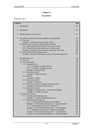
  • 1. Gripping IFRS Inventories Chapter 4 Inventories Reference: IAS 2 Contents: Page 1. Introduction 137 2. Definitions 137 3. Different classes of inventories 137 4. Recording inventory movement: periodic versus perpetual 138 4.1 Overview 138 Example 1: perpetual versus periodic system 138 4.2 Stock counts, inventory balances and stock theft 139 4.2.1 The perpetual system and the use of stock counts 139 4.2.2 The periodic system and the use of stock counts 139 Example 2: perpetual versus periodic system and stock theft 140 4.3 Gross profit and the trading account 141 Example 3: perpetual and periodic system: stock theft and profits 142 5. Measurement: cost 144 5.1 Overview 144 5.2 Cost of purchase 144 5.2.1 Transport costs 144 5.2.1.1 Transport/ carriage inwards 145 5.2.1.2 Transport/ carriage outwards 145 Example 4: transport costs 145 5.2.2 Transaction taxes 146 Example 5: transaction taxes 146 5.2.3 Rebates 147 Example 6: rebates 147 5.2.4 Discount received 148 Example 7: discounts 148 5.2.5 Finance costs due to extended settlement terms 149 Example 8: extended settlement terms 149 5.2.6 Imported inventory 151 Example 9: exchange rates – a basic understanding 151 Example 10: foreign exchange 152 5.3 Cost of conversion 153 5.3.1 Variable manufacturing costs 153 Example 11: variable manufacturing costs 153 5.3.2 Fixed manufacturing costs 154 5.3.2.1 Under-production and under-absorption 154 Example 12: fixed manufacturing costs – under-absorption 154 5.3.2.2 Over-production and over-absorption 156 Example 13: fixed manufacturing costs – over-absorption 156 5.3.2.3 Budgeted versus actual overheads summarised 157 Example 14: fixed manufacturing costs – over-absorption 158 Example 15: fixed manufacturing costs – under-absorption 159 135 Chapter 4
  • 2. Gripping IFRS Inventories Contents continued … Page 6. Measurement: cost formulas (inventory movements) 160 6.1 Overview 160 6.2 First-in-first-out method (FIFOM) 161 Example 16: FIFOM purchases 161 Example 17: FIFOM sales 161 Example 18: FIFOM sales 162 6.3 Weighted average method (WAM) 162 Example 19: WAM purchases 162 Example 20: WAM sales 163 6.4 Specific identification method (SIM) 163 Example 21: SIM purchases and sales 163 7. Measurement of inventories at year-end 164 7.1 Overview 164 Example 22: lower of cost or net realisable value 164 Example 23: lower of cost or net realisable value 165 Example 24: lower of cost or net realisable value 166 7.2 Testing for possible write-downs: practical applications 167 Example 25: lower of cost or net realisable value – with disclosure 168 8. Disclosure 171 8.1 Accounting policies 171 8.2 Statement of financial position and supporting notes 171 8.3 Statement of comprehensive income and supporting notes 171 Example 26: disclosure of cost of sales and depreciation 171 8.4 Sample disclosure involving inventories 172 8.4.1 Sample statement of financial position and related notes 172 8.4.2 Sample statement of comprehensive income and related notes 172 8.4.2.1 Costs analysed by nature in the statement of comprehensive income 172 8.4.2.2 Costs analysed by function in the statement of comprehensive income 173 8.4.2.3 Costs analysed by function in the notes to the statement of comprehensive income 173 9. Summary 175 136 Chapter 4
  • 3. Gripping IFRS Inventories 1. Introduction The topic of inventories is an important area for most companies and thus an important section to properly understand. The issues regarding inventories include: • when to recognise the acquisition of inventory, • how to measure the initial recognition, • how to measure inventory subsequently (year-ends and when sold), • derecognition of inventory when it is sold or scrapped, • disclosure of inventories in the financial statements. 2. Definitions Inventories are assets that are (IAS 2.6): • held for sale in the ordinary course of business; or • in the process of production for such sale; or • in the form of materials or supplies to be consumed in the production process or in the rendering of services. Net realisable value is (IAS 2.6): • the estimated selling price in the ordinary course of business; • less the estimated costs of completion; and • less the estimated costs necessary to make the sale. Fair value is (IAS 2.6): • the amount for which an asset could be exchanged, or a liability settled, • between knowledgeable, willing parties in an arm’s length transaction. The difference between a fair value and a net realisable value is essentially as follows: • a fair value is what is referred to as an non-entity-specific value, since it is determined by market forces; whereas • a net realisable value is what is referred to as an entity-specific value because it is affected by how the entity plans to sell the asset. 3. Different classes of inventories The type or types of inventories that an entity may have depends largely on the type of business: retail, manufacturer and service providers, being the most common types. If the entity runs a retail business, then the inventory will generally be called: merchandise. A manufacturing business will generally call his inventory: • finished goods; • work-in-progress; and • raw materials. Another type of inventory held by many types of businesses (e.g. retail, manufacturer and service provider) includes fuel, cleaning materials and other incidentals, often referred to as: • consumable stores. A business may, of course, have any combination of the above types of inventory. 137 Chapter 4
  • 4. Gripping IFRS Inventories 4. Recording inventory movements: periodic versus perpetual 4.1 Overview Inventory movements may be recognised using either the perpetual or periodic system. The perpetual system refers to the constant updating of both the inventory and cost of sales accounts for each purchase and sale of inventory. The balancing figure will represent the value of inventory on hand at the end of the period. This balance is checked by performing a stock count at the end of the period (normally at year-end). The periodic system simply accumulates the total cost of the purchases of inventory in one account, (the purchases account), and updates the inventory account on a periodic basis (often once a year) through the use of a physical stock count. The balancing figure, in this case, is the cost of sales. Example 1: perpetual versus periodic system C Opening inventory balance 55 000 Purchases during the year (cash) 100 000 A stock count at year-end reflected 18 000 units on hand (cost per unit: C5). Required: Show the t-accounts using A. the perpetual system assuming that 13 000 units were sold during the year; and B. the periodic system. Solution to example 1A: using the perpetual system Inventory (Asset) Cost of Sales (Expense) O/ balance 55 000 Cost of sales (2) 65 000 Inventory (2) 65 000 Bank (1) 100 000 C/ balance c/f 90 000 155 000 155 000 C/ balance (3) 90 000 (1) The cost of the purchases is debited directly to the inventory (asset) account. (2) The cost of the sale is calculated: 13 000 x C5 = C65 000 (since the cost per unit was constant at C5 throughout the year, the cost of sales would have been the same irrespective of whether the FIFO, WA or SI method was used). (3) The final inventory on hand at year-end is calculated as the balancing figure by taking the opening balance plus the increase in inventory (i.e. purchases) less the decrease in inventory (i.e. the cost of the sales): 55 000 + 100 000 – 65 000 = 90 000. This is then compared to the physical stock count that reflected that the balance should be 90 000. No adjustment was therefore necessary. Solution to example 1B using the periodic system Purchases Trading Account Bank (2) 100 000 T/ account(5) 000 Inventory o/b(3) 55 Inventory c/b(4) 90 000 000 Purchases (5) 000 Total c/f (6) 65 000 155 000 155 000 Total b/f (6) 65 000 138 Chapter 4
  • 5. Gripping IFRS Inventories Inventory (Asset) O/ balance(1) 55 000 T/ account(3) 000 T/ account(4) 90 000 This balance will remain as C55 000 for the entire period until such time as the stock count is performed. (1) The purchases are recorded in the purchases account during the period (this account will be closed off at the end of the period to the trading account). (2) The closing balance of the inventory account is determined at the end of the period by physically counting the inventory on hand and valuing it (C90 000). In order for the closing balance to be recorded, the opening balance of C55 000 needs to first be removed from the asset account by transferring it to the trading account. (3) The inventory is counted and valued via a physical stock count (which is typically performed on the last day of the period, being the end of the reporting period). This figure is debited to the inventory account with the credit-entry posted to the trading account: given as C90 000 (4) The total of the purchases during the period is transferred to the trading account. (5) Notice how the trading account effectively records the cost of sales and that the cost of sales is the same as if the perpetual system had been used instead: 65 000. Incidentally, the inventory balance is also the same, irrespective of the method used: 90 000. 4.2 Stock counts, inventory balances and stock theft In example 1, the cost of sales and inventory balances are not affected by whether the periodic or perpetual system is used (i.e. cost of sales was C65 000 and inventory was C90 000 in part A and part B). This may not always be the case however, since a disadvantage of the periodic system is that any stock thefts will remain undetected. The periodic system is, however, still useful to small businesses due to its practical simplicity. 4.2.1 The perpetual system and the use of stock counts When using the perpetual system, the accountant is able to calculate the balance on the inventory account without the use of a stock count. This balance, however, reflects what the balance should be – not necessarily what the actual balance is. A sad truth of our society is that it is plagued by theft. Therefore, even though the accountant is not reliant on the stock count, a stock count is performed as a control measure. In other words, the balance calculated by the accountant is checked by performing a stock count at the end of the period (normally at year-end). If the physical count reveals a lower stock level than is reflected by the balance on the inventory account, the difference will be accounted for as a stock theft (expense) (if the physical count reflects more stock than appears in the inventory account, then this suggests that an error may have occurred in recording the purchases or sales during the period). 4.2.2 The periodic system and the use of stock counts When using the periodic system, the accountant does not have any idea of what his cost of sales are until the stock count is performed. Since we are using the stock count to calculate the cost of sales, the accountant will also not have an idea of what the inventory balance should be (if we had the cost of sales figure, we could have calculated the closing balance as: opening balance + purchases – cost of sales). In short: when using the periodic system, the accountant is unable to calculate the balance on the inventory account without the use of a stock count. If the accountant does not know what the balance should be, the stock count will not be able to highlight any stock thefts. 139 Chapter 4
  • 6. Gripping IFRS Inventories The fact that any stock thefts will remain undetected if the periodic system is used is shown in this next example. Example 2: perpetual versus periodic system and stock theft C Units Opening inventory balance 55 000 11 000 Purchases during the year (cash) 100 000 20 000 A stock count at year-end reflected 16 000 units on hand (cost per unit: C5). Required: Show the t-accounts using A. the perpetual system assuming that the company sold 13 000 units during the year; and B. the periodic system. Solution to example 2A using the perpetual system and stock theft Inventory (Asset) Cost of sales (Expense) O/ balance 55 Cost of S 65 000 Inventory (2) 65 000 (2) 000 Bank (1) 100 Subtotal 90 000 000 c/f 155 155 000 000 Subtotal (3) 90 Cost of 10 000 000 T(4) C/ bal c/f 80 000 90 90 000 000 C/ 80 balance(5) 000 Cost of theft (Expense) Inventory (4) 10 000 (1) The cost of the purchases is debited directly to the inventory (asset) account. (2) The cost of the sale is calculated: 13 000 x C5 = C65 000 (since the cost per unit was constant at C5 throughout the year, the cost of sales would have been the same irrespective of whether the FIFO, WA or SI method was used). If the business has very few sales or has a sophisticated system, the inventory and cost of sales accounts are updated immediately for each sale that takes place. This example processes the cumulative sales for the year. (3) The final amount of inventory that should be on hand at year-end is calculated as the balancing figure by taking the opening balance plus the increase in inventory (i.e. purchases) less the decrease in inventory (i.e. the cost of the sales): 55 000 + 100 000 – 65 000 = 90 000 (4) A stock count is performed and whereas there should have been 18 000 units on hand at year-end (11 000 + 20 000 – 13 000 units), there are only 16 000 units. It is therefore clear that 2 000 units have been stolen. The cost of this theft is therefore 10 000 (2 000 x C5). (5) The closing balance of inventory must reflect the reality and therefore the balance has been reduced from what it should have been (90 000) to what it is (80 000). 140 Chapter 4
  • 7. Gripping IFRS Inventories Solution to example 2B using the periodic system and stock theft Purchases Trading Account Bank (2) 100 000 T/account(5) 100 000 Inventory o/b(3) 55 Inventory c/b (4) 80 000 000 Purchases (5) 000 Total c/f (6) 75 000 155 000 155 000 Total b/f (6) 75 000 Inventory (Asset) O/ balance(1) 55 000 Trade a/c(3) 000 Trade a/c(4) 80 000 (1) This balance will remain as C55 000 for the entire period until such time as the stock count is performed. (2) The purchases are recorded in the purchases account during the year (this account will be closed off at the end of the period to the trading account). (3) The closing balance of the inventory account is determined at the end of the period by physically counting the inventory on hand and valuing it (C90 000). In order for the closing balance to be recorded, the opening balance of C55 000 needs to first be removed from the asset account by transferring it to the trading account. (4) The inventory is counted and valued via a physical stock count (which is typically performed at the end of the reporting period). This figure is debited to the inventory account with the credit-entry posted to the trading account: C80 000 (16 000 x C5). (5) The total of the purchases during the period is transferred to the trading account. (6) The trading account effectively records the cost of sales. Whereas the perpetual system in Part A indicated that cost of sales was 65 000 and that there was a cost of theft of 10 000, this periodic system indicates that cost of sales is 75 000. In other words, the periodic system assumed that all missing stock was sold. It is therefore less precise in describing its expense but it should be noted that the total expense is the same under both systems (periodic: 75 000 and perpetual: 65 000 + 10 000). Incidentally, the inventory balance is the same under both methods: 80 000. 4.3 Gross profit and the trading account If one uses the periodic system, the trading account is first used to calculate cost of sales. The sales account is then also closed off to the trading account, at which point the total on the trading account (sales – cost of sales) equals the gross profit (or gross loss). This total is then transferred to (closed off to) the profit and loss account together with all other income and expense accounts. The total on the profit and loss account will therefore equal the final profit or loss for the year. If the perpetual system is used, the trading account is only used to calculate gross profit: it is not used to calculate cost of sales. The cost of sales account and sales account are transferred to (closed off to) the trading account. The total on this trading account (sales – cost of sales) represents the gross profit. This total will be transferred to (closed off to) the profit and loss account together with all other income and expense accounts. The total on the profit and loss account will therefore equal the final profit or loss for the year. The gross profit calculated according to the perpetual system may differ from that calculated under the periodic system if, for example, stock theft went undetected. The final profit or loss calculated in the profit and loss account will, however, be the same. 141 Chapter 4
  • 8. Gripping IFRS Inventories The use of the trading account to calculate gross profit and how gross profits can differ is shown in this next example. Example 3: perpetual and periodic system: stock theft and profits C Units Opening inventory balance 55 000 11 000 Purchases during the year (cash) 100 000 20 000 A stock count at year-end reflected 16 000 units on hand (cost per unit: C5). Revenue from sales totalled C95 000 for the period (cash). Required: Show the ledger accounts and extracts of the statement of comprehensive income using: A. the perpetual system assuming that the company sold 13 000 units during the year; and B. the periodic system assuming that sales totalled C95 000. Solution to example 3A: perpetual system: stock theft and profits Inventory (Asset) Cost of sales (Expense) O/ balance 55 000 Cost of S 65 000 Inventory 65 000 TA (1) 65 000 Bank 100 Subtotal 90 000 000 c/f 155 155 000 000 Subtotal 90 000 Cost of T 10 000 b/f C/ bal c/f 80 000 90 000 90 000 C/ balance 80 000 Cost of theft (Expense) Inventory 10 000 P&L (3) 10 000 Sales (Income) Trade Acc 95 000 Bank 95 000 (1) Trading account (Closing account) Profit and loss account (Closing account) CoS (1) 65 Sales (1) 95 Cost: theft (3) 10 000 Trade A/c 30 000 000 000 (GP) (2) P&L (2) 30 Total c/f 20 000 000 95 95 30 000 30 000 000 000 Total b/f 20 000 (4) (1) Sales and cost of sales are transferred to the trading account. (2) The total on the trading account (gross profit) is transferred to the profit and loss account. (3) All other income and expenses are closed off at the end of the year to the profit and loss account. 142 Chapter 4
  • 9. Gripping IFRS Inventories (4) If there were no other income and expense items, then this total represents the final profit for the year. It would then be transferred to the equity account: retained earnings. Company name Statement of comprehensive income For the period ended …. (extracts) CY PY C C Revenue from sales 95 000 x Cost of sales (65 000) (x) Gross profit 30 000 x Cost of theft (10 000) (x) Profit before considering other income and 20 000 x expenses Solution to example 3B: periodic system: stock theft and profits Inventory (Asset) Sales (Income) O/ 55 000 TA 55 000 TA (2) 95 000 Bank 95 000 balance TA 80 000 Purchases Bank 100 TA 100 000 000 Trading account (Closing account) Profit and loss account (Closing account) Inv o/bal 55 000 Inv c/bal 80 000 TA (GP) (3) 20 000 Purchases 100 Total c/f 75 000 000 155 155 000 000 Total b/f 75 000 Sales (2) 95 000 (1) P&L (3) 20 000 95 000 95 000 (1) The total brought forward on the trading account represents the cost of inventory (assumed to be cost of sales). (2) Sales are credited to the trading account. (3) The balance on the trading account represents the gross profit and this is transferred to the profit and loss account. All other income and expense accounts are then also transferred to (closed off to) the profit and loss account. The profit and loss account therefore converts gross profit into the final profit for the period. Company name Statement of comprehensive income For the period ended …. (extracts) CY PY 143 Chapter 4
  • 10. Gripping IFRS Inventories C C Revenue from sales 95 000 x Cost of sales (75 000) (x) Gross profit (4) 20 000 x (4) Notice how the gross profit in the statement of comprehensive income is 20 000 under the periodic system but is 30 000 under the perpetual system. The final profit in both cases is, however, 20 000. 5. Measurement: cost (IAS 2.10) 5.1 Overview The costs that one should include in (i.e. capitalise to) inventory include the (IAS 2.10): • costs to purchase the inventory, • costs to convert the inventory into a saleable or consumable condition; and • other costs to bring the inventory to its present location and condition. 5.2 Cost of purchase (IAS 2.11) The cost of inventory would include all costs directly associated with the acquisition, such as: • purchase price, • transport costs (inwards), • import duties and transaction taxes that are not reclaimable * by the business, and • other direct costs. The following costs would be excluded from the cost of inventory: • import duties and transaction taxes that are reclaimable * by the business, • financing costs due to extended payment terms. *: The acquisition of inventory very often involves the payment of transaction taxes and import duties. Sometimes these taxes or import duties (which are either paid over to the supplier or directly to the tax authority) and are able to be reclaimed at a later date from the tax authorities. If they can be reclaimed (recovered), then there is no net cost to the business. A typical example is the transaction tax levied by many countries: VAT. See chapter 3 for more information in this regard. The following would be set-off against the cost of inventory: • rebates received, • trade, bulk and cash discounts received, • settlement discounts received or expected to be received. Only those costs that are incurred in bringing the inventory to its present location and condition may be capitalised. The following costs should therefore always be expensed: • abnormal amounts of wastage; • storage costs (unless these are directly attributable to the production process, e.g. the cost of storage in-between processes that is considered to be unavoidable and normal); and • selling costs. 5.2.1 Transport Costs There are two types of transport costs (carriage costs): transport inwards and transport outwards, each of which being accounted for differently. 5.2.1.1 Transport/ carriage inwards The cost of transport inwards refers to the cost of transporting the purchased inventory from the supplier to the purchaser’s business premises. It is a cost that was incurred in ‘bringing the inventory to its present location’ and should therefore be included in the cost of inventory. 144 Chapter 4
  • 11. Gripping IFRS Inventories 5.2.1.2 Transport/ carriage outwards Frequently, when a business sells its inventory, it offers to deliver the goods to the customer’s premises. The cost of this delivery is referred to as ‘transport outwards’. It is a cost that is incurred in order to complete the sale of the inventory rather than to purchase it and may therefore not be capitalised (since it is not a cost that was incurred in ‘bringing the inventory to its present location’). Transport outwards should, therefore, be recorded as a selling expense in the statement of comprehensive income instead of capitalising it to the cost of the inventory. Example 4: transport costs A company purchases inventory for C100 from a supplier. No VAT was charged. The following additional information is provided: Cost of transport inwards C25 Cost of transport outwards C15 All amounts were on credit and all amounts owing were later paid in cash. Required: Calculate the cost of the inventory and show all related journal entries. Solution to example 4: transport costs Calculation Cost of inventory purchased: 100 + 25 = C125 Journals Debit Credit Inventory (A) 125 Trade payable (L) 125 Cost of inventory purchased on credit: 100 + 25 (transport inwards) Transport outwards (E) 15 Trade payable (L) 15 Cost of delivering inventory to the customer Trade payable (L) 100 Bank 100 Payment of supplier Trade payable (L) 25 Bank 25 Payment of the transport company that transported goods from supplier Trade payable (L) 15 Bank 15 Payment of the transport company that transported goods to the customer 5.2.2 Transaction taxes The only time that transaction taxes (e.g. VAT) or import duties will form part of the cost of inventory is if they may not be claimed back from the tax authorities. This happens, for 145 Chapter 4
  • 12. Gripping IFRS Inventories example, where the entity fails to meet certain criteria laid down by the tax authority (e.g. if the entity is not registered as a vendor for VAT purposes). Example 5: transaction taxes An entity purchased inventory. The costs thereof were as follows: C Total invoice price (including 14% VAT) paid in cash to the supplier 9 120 Import duties paid in cash directly to the country’s Customs 5 000 Department Required: Show the ledger accounts assuming: A. The VAT and the import duties were refunded by the tax authorities one month later. B. The VAT and the import duties will not be refunded. Solution to example 5A: refundable taxes and import duties Inventory (Asset) VAT receivable (Asset) Bank (1) (5) 8 000 Bank (1) 1 120 Bank (3) 1 120 Bank Import duties receivable (Asset) VAT 1 120 Inv & VAT 9 Bank (2) 5 000 Bank (4) 5 000 receivable (3) Receivable (1) 120 Import duties 5 000 Import 5 recoverable (4) duties 000 recoverable (2) (1) The VAT portion of the invoice price must be separated and recognised as a receivable since the entity will claim this VAT back: 9 120 / 114 x 14 = 1 120. The balance of the invoice price is recognised as inventory since this represents the real cost to the entity: 9 120 / 114 x 100 = 8 000 (2) The import duties payable directly to the Customs Department were also refundable and therefore the entire import duty paid is recognised as a receivable. This can happen where, for example, another country in which the entity operates offers a dispensation whereby it refunds certain taxes paid by the entity to other countries. (3) VAT refund received. (4) Import duty refund received. (5) Notice that the inventory account reflects C8 000 and that equals net amount paid per the bank account is also C8 000: 9 120 + 5 000 – 1 120 – 5 000. Solution to example 5B: non-refundable taxes and import duties Inventory (Asset) Bank Bank (1) 9 120 Inv (1) 9 120 Bank (2) 5 000 IDR (2) 5 000 14 14 120 120 (1) The VAT portion of the invoice price is not separated since none of it is refundable. (2) The import duties payable directly to the Customs Department were not refundable and are therefore part of the costs of acquiring the inventory. 146 Chapter 4
  • 13. Gripping IFRS Inventories (3) Notice that the inventory account reflects a balance of C14 120 and that this equals the amount paid per the bank account: 9 120 + 5 000. 5.2.3 Rebates The entity that is purchasing inventory may receive a rebate that is somehow related to the inventory. There are many different types of rebates possible. The rule is, however, that if the rebate is received as a reduction in the purchase price, then the cost of the inventory must be reduced by the rebate. Some rebates, although connected to the inventory, are not really a direct reduction in the purchase price but a refund of certain of the entity’s costs. In this case, the rebate received should be recognised as income instead. Example 6: rebates An entity purchased inventory for cash. The details thereof were as C follows: • Invoice price (no VAT is charged on these goods) 9 000 • Rebate offered to the entity by the supplier 1 000 Required: Show the ledger accounts assuming that the terms of the agreement made it clear that the rebate: A. Was a reduction to the invoice price of the inventory; and B. Was a refund of the entity’s expected selling costs. Solution to example 6A: rebate reducing cost of inventory Inventory (Asset) Bank Bank (1) 8 000 Inv (1) 8 000 (1) The rebate reduces the cost of inventory: 9 000 – 1 000 Solution to example 6B: rebate not reducing cost of inventory Inventory (Asset) Bank (1) Bank 9 000 Inv (1) 8 000 Rebate received (Income) Bank (1) 1 000 (1) The cost of inventory is shown at 9 000 even though only 8 000 is paid. This is because the rebate of C1 000 is not connected to the cost of the inventory but the entity’s future expected selling costs. The rebate is recognised as income instead because by recognising it as income, it enables the rebate income to be matched with the related selling expenses. 5.2.4 Discount received There are a variety of discounts that you could receive on the purchase of goods: 147 Chapter 4
  • 14. Gripping IFRS Inventories • trade discount or bulk discount : this is usually received after successfully negotiating the invoice price down, because you are a regular customer or you are buying in bulk; and • cash discount : this is sometimes received as a ‘reward’ for paying in cash; • settlement discount: this is sometimes received as a ‘reward’ for paying promptly. All these discounts are deducted from the cost of the inventory. Trade discounts, bulk discounts and cash discounts are generally agreed to on the transaction date. Settlement discounts, however, will have to be estimated on the transaction date based on when the entity expects to settle its account with the creditor. Example 7: discounts An entity purchased inventory. The costs thereof were as follows: C • Marked price (no VAT is charged on these goods) 9 000 • Trade discount 1 000 Required: Show the ledger accounts assuming: A. The entity pays in cash on transaction date and receives a cash discount of C500; and B. The supplier offers an early settlement discount of C400 if the account is paid within 20 days: the entity pays within the required period of 20 days. C. The supplier offers an early settlement discount of C400 if the account is paid within 20 days: the entity pays after a period of 20 days. Solution to example 7A: discounts including a cash discount Inventory (Asset) Bank (1) Bank 7 500 Inventory 7 500 (1) 1) The marked price is reduced by the trade discount and the cash discount: 9 000 – 1 000 – 500 Solution to example 7B: discounts including a settlement discount Inventory (Asset) Trade payables (Liability) Bank (1) 7 600 Bank (2) 7 600 Inventory 8 000 (1) Sett Disc 400 All (3) Bank Settlement discount allowance (negative liability) Tr Payable 7 Inventory 400 Tr Payable 400 (2) (1) (3) 600 (1) The marked price is reduced by the trade discount and the estimated settlement discount: 9 000 – 1 000 – 400 = 7 600. The settlement discount is an estimated discount until the payment is made within the required period, at which point the discount becomes an actual discount received. Until then, the creditor’s account is credited with the full amount payable and an allowance for possible settlement discount of C400 is debited (this reduces the carrying amount of the creditors presented in the statement of financial position). (2) The entity pays within 20 days and the settlement discount becomes a reality (i.e. the estimated discount becomes an actual discount). The payment is therefore only C7 600. 148 Chapter 4
  • 15. Gripping IFRS Inventories (3) Since the creditor is paid within the required settlement period, the entity earned its settlement discount. The settlement discount allowance is thus reversed to the creditors account (clears the balance owing to nil). Solution to example 7C: discounts including a settlement discount Inventory (Asset) Trade payables (Liability) Bank (1) 7 600 Bank (2) 8 Inventory 8 000 000 (1) Bank Settlement discount allowance (negative liability) Tr Payable 8 Inv (1) 400 Fin exp (3) 400 (2) 000 Finance expense Sett Disc 400 All (3) (1) The marked price is reduced by the trade discount and the estimated settlement discount: 9 000 – 1 000 – 400 = 7 600. The settlement discount is an estimated discount until the payment is made within the required period, at which point the discount becomes an actual discount received. Until then, the creditor’s account is credited with the full amount payable and an allowance for possible settlement discount of C400 is debited (this reduces the carrying amount of the creditors presented in the statement of financial position). (2) The entity pays after 20 days and the settlement discount is forfeited. The payment is therefore C8 000. (3) Since the creditor is not paid within the required settlement period, the entity lost its settlement discount. The settlement discount allowance is thus recognised as an expense. 5.2.5 Finance costs due to extended settlement terms Instead of paying in cash on transaction date or paying within a short period of time, an entity could choose to pay over a long period of time. Instead of receiving a discount and thus decreasing the cash outflow, this choice would increase the cash outflow. The time value of money must be taken into consideration when estimating the fair value of the cost and the cost of paying over an extended period of time must be reflected as an interest expense. This applies in all cases where the effect of the time value of money is considered to be material. Example 8: extended settlement terms An entity purchased inventory on 1 January 20X1. The costs thereof were as follows: • Invoice price payable on 31 December 20X2 C6 050 • Market interest rate 10% Required: Show the journal entries assuming: A. The effect of the time value of money is not considered to be material; and B. The effect of the time value of money is considered to be material. Solution to example 8A: extended settlement terms: immaterial effect 1 January 20X1 Debit Credit 149 Chapter 4
  • 16. Gripping IFRS Inventories Inventory (A) 6 050 Trade payable (L) 6 050 Cost of inventory purchased on credit (time value ignored because effects immaterial to the company) 31 December 20X2 Trade payable (L) 6 050 Bank 6 050 Payment for inventory purchased from X on 1 January 20X1 (2 years ago) Solution to example 8B: extended settlement terms: material effect The cost of the inventory must be measured at the present value of the future payment (thereby removing the finance costs from the cost of the purchase, which must be recognised as an expense). The present value can be calculated using a financial calculator by inputting the repayment period (2 years), the future amount (6 050) and the market related interest rate (10%) and requesting it to calculate the present value. (FV = 6 050, i = 10, n = 2, COMP PV) This can also be done without a financial calculator, by following these steps: Step 1: calculate the present value factors Present value factor on due date 1.00000 Present value factor one year before payment is 1 / (1+10%) 0.90909 due Present value factor two years before payment is 0.90909 / (1 + 10%) or 0.82645 due 1 / (1 + 10%) / (1 + 10%) Step 2: calculate the present values Present value on transaction 6 050 x 0.82645 (2 years before payment is 5 000 date due) Present value one year later 6 050 x 0.90909 (1 year before payment is 5 500 due) Present value on due date Given: future value (or 6 050 x 1) 6 050 The interest and balance owing each year can be calculated using an effective interest rate table: Year Opening balance Interest expense Payments Closing balance 20X1 5 000 Opening PV 500 5 000 x 10% (0) 5 500 5 000 + 500 20X2 5 500 550 5 500 x 10% (6 050) 0 5 500 + 550 – 6050 1 050 (6 050) Notice that the present value is 5 000 and yet the amount paid is 6 050. The difference between these two amounts is 1 050, which is recognised as interest expense over the two years. 1 January 20X1 Debit Credit Inventory (A) 5 000 Trade payable (L) * 5 000 150 Chapter 4
  • 17. Gripping IFRS Inventories Cost of inventory purchased on credit (invoice price is 6 050, but recognised at present value of future amount). 10% used to discount the future amount to the present value: 6 050 / 1.1 / 1.1 or 6 050 x 0.82645 31 December 20X1 Interest expense 500 Trade payable (L) * 500 Effective interest incurred on present value of creditor: 5 000 x 10% 31 December 20X2 Debit Credit Interest expense 550 Trade payable (L) * 550 Effective interest incurred on present value of creditor: 5 500 x 10% Trade payable (L) 6 050 Bank 6 050 Payment of creditor: 5 000 + 500 + 550 * Notice that the trade payable balance: • At 1 January 20X1 (2 years before payment is due) is 5 000. This is calculated using the ‘present value factor for two years’: 6 050 x 0.82645 = 5 000, • At 31 December 20X1 (1 year before payment is due) is 5 500 (5 000 + 500). This can be checked by using the ‘present value factor after 1 year’ of 0.90909: 6 050 x 0.90909 = 5 500. • At 31 December 20X2 (immediately before payment) is 6 050 (5 000 + 500 + 550). This can be checked using the ‘present value factor for now’ of 1: 6 050 x 1 = 6 050 5.2.6 Imported inventory When inventory is purchased from a foreign supplier the goods are referred to as being ‘imported’. A complication of an imported item is that the cost of the goods purchased is generally denominated in a foreign currency on the invoice. This foreign currency amount must be converted into the local currency using the currency exchange rate ruling on transaction date. Example 9: exchange rates – a basic understanding Mr. X has $1 000 (USD) that he wants to exchange into South African Rands (R). Required: Calculate the number of Rands he will receive if the exchange rate ruling on the date he wants to exchange his dollars for Rands is: A. R5: $1 (direct method); and B. $0.20: R1 (indirect method). Solution to example 9A: exchange rates – dollar is the base $1 000 x R5 / $1 = R5 000 (divide by the currency you’ve got and multiply by the currency you want) Solution to example 9B: exchange rates – Rand is the base $1 000 x R1 / $0.20 = R5 000 (divide by the currency you’ve got and multiply by the currency you want) Since currency exchange rates vary daily, it is very important to identify the correct transaction date since this will determine both when to recognise the purchase and what exchange rate to use when measuring the cost of the inventory. 151 Chapter 4
  • 18. Gripping IFRS Inventories The transaction date for an imported asset is determined using the same principles used had the asset been purchased locally: when the risks and rewards of ownership are transferred. There are two common ways of purchasing goods from a foreign supplier: on a ‘customs, insurance and freight’ basis (CIF) or a ‘free on board’ basis (FOB). The difference between the two affects the date on which risks and rewards are transferred and thus determine the transaction date. Although the terms of the agreement must always be thoroughly investigated first, the general rule is that: • if goods are purchased on a FOB basis, the risks and rewards are transferred as soon as the goods are loaded onto the ship at the foreign port; and • if goods are purchased on a CIF basis, the risks and rewards are transferred only when the goods arrive safely in the local harbour and are released from customs. In summary: goods purchased from a foreign supplier will be recorded by the purchaser, by converting the foreign currency into what is called the reporting entities functional currency (generally his local currency), using the spot exchange rate ruling on the transaction date. Any change in the spot exchange rate thereafter is generally recognised in profit or loss (i.e. is recognised as an expense or income and not recognised as an adjustment to the inventory asset account). Example 10: foreign exchange A company in South Africa purchases $100 000 of raw materials from a supplier in America. The following are the spot rates (rates of exchange on a particular date): Date: R: $1 1 January 20X2 R7,20:$1 15 February 20X2 R7,30: $1 15 March 20X2 R7,50: $1 The goods are loaded onto the ship in New York on 1 January 20X2 and are released from the Customs Department at the Durban harbour (South Africa) on 15 February 20X2. The company pays the American supplier on 15 March 20X2. The currency of South Africa is rands (R) and the currency of America is dollars ($). Required: Calculate the cost of inventory and the foreign exchange gain or loss and show the related journal entries, assuming the following: A. The goods are purchased FOB. B. The goods are purchased CIF. Solution to example 10A: foreign exchange – FOB 1 January 20X2 Debit Credit Inventory (A) $100 000 x 7,20 = R720 000 720 000 Creditor (foreign) 720 000 Purchase of inventory from New York 15 March 20X2 Foreign exchange loss ($100 000 x 7,50) – 720 000 30 000 Creditor (foreign) 30 000 Translation of foreign creditor on payment date: Creditor (foreign) 720 000 + 30 000 or $100 000 x 750 000 7.50 Bank 750 000 Payment of foreign creditor Solution to example 10B: foreign exchange – CIF 15 February 20X2 Debit Credit 152 Chapter 4
  • 19. Gripping IFRS Inventories Inventory (A) $100 000 x 7,30 = R730 000 730 000 Creditor (foreign) 730 000 Purchase of inventory from New York 15 March 20X2 Foreign exchange loss ($100 000 x 7,50) – 730 000 20 000 Creditor (foreign) 20 000 Translation of foreign creditor on payment date Creditor (foreign) 730 000 + 20 000 or $100 000 x 750 000 7.50 Bank 750 000 Payment of foreign creditor Notice: The amount paid under both situations is R750 000 (using the spot rate on payment date). The inventory is, however, measured at the spot rate on transaction date: the transaction dates differed between part A (FOB) and part B (CIF) and therefore the cost of inventory differs in part A and part B. The movement in the spot rate between transaction date and payment date is recognised in profit and loss (i.e. not as an adjustment to the inventory asset account). 5.3 Cost of conversion (IAS 2.12 - .14) Manufactured inventory on hand at the end of the financial period must be valued at the total cost of manufacture, being not only the cost of purchase of the raw materials but also the cost of converting the raw materials into a finished product, including: • direct and indirect costs of manufacture; and • any other costs necessarily incurred in order to bring the asset to its present location and condition (where even administrative overheads could be included if it can be argued that they contributed to bringing the asset to its present condition and location). Apart from the need to know the total manufacturing cost to debit to the inventory account, it is also important to know what the manufacturing cost per unit is when quoting customers. Manufacturing costs (direct and indirect) may be divided into two main categories: • variable costs: these are costs that vary directly or almost directly with the level of production e.g. raw materials (a direct cost that varies directly), labour and variable overheads (indirect costs that vary directly or almost directly); and • fixed costs: these are indirect costs that do not vary with the level of production e.g. factory rental, depreciation and maintenance of factory buildings. 5.3.1 Variable manufacturing costs Variable costs increase and decrease in direct proportion (or nearly in direct proportion) to the number of units produced (or level of production). By their very nature it is easy to calculate the variable cost per unit. Example 11: variable manufacturing costs Assume that one unit of inventory manufactured uses: • 3 labour hours (at C3 per hour) and • 1 kilogram of raw material X (at C2 per kg excluding VAT). Required: A. Calculate the variable manufacturing cost per unit of inventory. B. Show the journal entries for the manufacture of 10 such units assuming that the labour is paid for in cash and assuming that the raw materials were already in stock. Assume further that the 10 units were finished. Solution to example 11: variable manufacturing costs Calculation: variable manufacturing cost per unit C 153 Chapter 4
  • 20. Gripping IFRS Inventories Direct labour: 3 hours x C3 9 Direct materials: 1 kg x C2 2 Variable manufacturing cost per unit 11 Journals Debit Credit Inventory: work-in-progress 90 Bank 90 Cost of manufacture of 10 units: labour cost paid in cash (10 x C9) Inventory: work-in-progress 20 Inventory: raw materials 20 Cost of manufacture of 10 units: raw materials used (10 x C2) Journals continued … Debit Credit Inventory: finished goods 110 Inventory: work-in-progress 110 Completed units transferred to finished goods (10 units x C11): 90 + 20 5.3.2 Fixed manufacturing costs It is not as easy to calculate the fixed manufacturing cost per unit. The cost of inventory needs to be known during the year for quoting purposes as well as for any reports needing to be provided during the year. Since the standard requires that the cost of inventory includes fixed manufacturing overheads, we need to calculate a fixed cost per unit, which we call the fixed manufacturing overhead application rate (FOAR). We won’t be able to calculate an accurate fixed cost per unit until the end of the year since we will only know the extent of the actual production at the end of the year. As mentioned above, however, a rate is needed at the beginning of the year for the purposes of quoting, budgeting and interim reporting. This means that a budgeted fixed overhead application rate (BFOAR) using budgeted normal production as the denominator, is calculated as an interim measure: Fixed manufacturing overheads Normal production The actual fixed overhead application rate (AFOAR), however, would depend on the actual level of inventory produced in any one period and can only be calculated at year-end. Fixed manufacturing overheads Greater of: actual and normal production 5.3.2.1 Under-production and under-absorption If the company produces at a level below budgeted production, a portion of the fixed overheads in the suspense account will not be allocated to the asset account. This unallocated overhead amount is termed an ‘under-absorption’ of fixed overheads and since it results from under-productivity, it refers to the cost of the inefficiency, which is quite obviously not an asset! This amount is expensed instead. Example 12: fixed manufacturing costs – under-absorption Fixed manufacturing overheads C100 000 Normal expected production (units) 100 000 Actual production (units) 50 000 Required: A. Calculate the budgeted fixed manufacturing overhead application rate; B. Calculate the actual fixed manufacturing overhead application rate; and 154 Chapter 4
  • 21. Gripping IFRS Inventories C. Journalise the fixed manufacturing costs. Solution to example 12A: budgeted fixed manufacturing overhead application rate = Fixed manufacturing overheads Budgeted production = C100 000 100 000 units = C1 per unit We use this C1 per unit when quoting to our customers and when drafting interim financial statements. Solution to example 12B: actual fixed manufacturing overhead application rate = Fixed manufacturing overheads Greater of: budgeted and actual production = C100 000 100 000 units = C1 per unit Explanation why the actual production could not be used in this example: The actual application rate is calculated using the normal budgeted production since, in this case, the budgeted production exceeded the actual production. If the actual production had been used it would result in inventory being overvalued: = Fixed manufacturing overheads Actual production = C100 000 50 000 units = C2 per unit Each unit would erroneously include fixed manufacturing costs of C2 instead of the normal C1 as a result of the company’s inefficiency! Bearing in mind that the Framework states that the value of an asset should represent the probable future economic benefits expected to flow from the asset, it does not make sense to show the cost of inventory at twice its normal value (C2 instead of C1) simply because the company was inefficient. Measuring the inventory using C2 would suggest that the future economic benefits are expected to double. Another way of looking at it is: if we used C2 per unit, the value of 50 000 units inventory would represent the full amount of fixed overheads incurred (C100 000) when only half of the required inventory was produced (therefore, only half of the fixed overheads should be included in the inventory account). Half the fixed overheads were wasted and therefore 50% x 100 000 should be expensed. The answer to this problem is to capitalise only the normal cost per unit (C1) to the inventory asset and expense the balance of the fixed manufacturing overheads (actual: C2 – normal: C1 = wastage: C1) as abnormal wastage of company resources. Solution to example 12C: fixed manufacturing overheads – journals During the year Debit Credit 155 Chapter 4
  • 22. Gripping IFRS Inventories Fixed manufacturing costs (Suspense account) 100 000 Bank/ Creditor 100 000 Fixed manufacturing overheads incurred: given Inventory (A) 50 000 Fixed manufacturing costs (Suspense account) 50 000 Allocation of fixed manufacturing overheads to inventory over the year: 50 000 x C1 (BFOAR) At year-end Fixed manufacturing overhead expense (E) (under-absorption) 50 000 Fixed manufacturing costs (Suspense account) 50 000 Expensing of the balance of the fixed manufacturing overhead suspense account at year-end: 100 000 (total paid) – 50 000 (capitalised) 5.3.2.2 Over-production and over-absorption If the company’s actual level of production exceeds budgeted production, the budgeted fixed overhead application rate per unit will be higher than the actual fixed overhead application rate per unit. If the budgeted application rate is used to absorb fixed overheads into the cost of the inventory during the course of the year, fixed manufacturing overheads will be ‘over- absorbed’ into the cost of inventory by the end of the year if the entity produced more units that were budgeted (over-production). This means that the asset will be overstated as the costs capitalised are not the actual costs incurred (i.e. will be shown at a value that exceeds cost) and will therefore need to be reduced. Example 13: fixed manufacturing costs – over-absorption Fixed manufacturing overheads C100 000 Normal expected production (units) 100 000 Actual production (units) 200 000 Required: A. Calculate the budgeted fixed manufacturing overhead application rate; B. Calculate the actual fixed manufacturing overhead application rate; and C. Journalise the fixed manufacturing costs. Solution to example 13A: budgeted fixed manufacturing overhead application rate = Fixed manufacturing overheads Budgeted production = C100 000 100 000 units = C1,00 per unit Solution to example 13B: actual fixed manufacturing overhead application rate = Fixed manufacturing overheads Greater of: budgeted and actual production = C100 000 200 000 units = C0.50 per unit Although we would have used the BFOAR of C1 per unit throughout the year for quoting our customers and for allocating fixed manufacturing costs to inventory during the period, the 156 Chapter 4
  • 23. Gripping IFRS Inventories final inventory balance would be valued using the actual cost (AFOAR) of C0.50 per unit instead. If the company valued their final inventory balance using the budgeted fixed overhead application rate of C1 instead, C200 000 of fixed overheads would have been included in inventory (C1 x 200 000 units). This is not allowed since the actual fixed overheads incurred were only C100 000 (IAS 2, which governs inventories, prohibits the measurement of inventory at above cost). Solution to example 13C: fixed manufacturing overheads - journal During the year Debit Credit Fixed manufacturing costs (suspense account) 100 000 Bank/ Creditor 100 000 Fixed manufacturing overheads incurred during the year: given Inventory (A) 200 000 x C1 (BFOAR) 200 000 Fixed manufacturing costs (suspense account) 200 000 Allocation of fixed manufacturing overheads to inventory over the year At year-end Fixed manufacturing costs (suspense account) (over-absorption) 100 000 Inventory (A) 100 000 Reversing the excess fixed manufacturing costs transferred to the inventory account (the suspense account will now have a zero balance) 5.3.2.3 Budgeted versus actual overhead rates summarised Budgeted production will seldom equal actual production and therefore the budgeted costs (BFOAR) per unit will generally not equal the actual costs (AFOAR) per unit. If, therefore, the budgeted fixed overhead absorption rate (BFOAR) is multiplied by the actual units produced, too much or too little of the overhead costs actually incurred are included in the inventory cost. The budgeted fixed overhead application rate is therefore calculated at: • the beginning of the year to measure the cost of inventory during the year; and then • at the end of the year to measuring the inventory balance. The budgeted fixed overhead application rate is calculated at the beginning of the year: Fixed manufacturing overheads BFOAR = Budgeted production The actual fixed overhead application rate (AFOAR) is calculated at the end of the year: Fixed manufacturing overheads AFOAR = Greater of: budgeted production and actual production In the event that actual production is greater than budgeted production, the actual fixed overhead application rate (AFOAR) is calculated using actual production since this avoids inventory being overvalued as a result of over-efficiency. In the event that actual production is less than budgeted production, the actual fixed overhead application rate is calculated using budgeted production, since this avoids inventory being overvalued as a result of company inefficiencies. Example 14: fixed manufacturing costs – over-absorption Budgeted production 1 000 units 157 Chapter 4
  • 24. Gripping IFRS Inventories Actual production 1 500 units Budgeted fixed non-manufacturing overheads C10 000 Budgeted fixed manufacturing overheads C40 000 Prime costs per unit C12 per unit Required: A. Calculate the budgeted fixed overhead application rate at the beginning of the year. B. Calculate the actual fixed overhead application rate at the end of the year. C. Show the entries in the related t-accounts. Solution to example 14A: budgeted fixed manufacturing overheads rate (AP > BP) = Fixed manufacturing overheads Budgeted production = C40 000 1 000 units = C40 per unit Solution to example 14B: actual fixed manufacturing overheads rate (AP > BP) = Fixed manufacturing overheads Greater of: budgeted production and actual production = C40 000 1 500 units = C26,67 per unit Solution to example 14C: t-accounts (AP > BP) Bank Fixed manufacturing overheads (Suspense) FOE (1) 10 Bank (2) 40 000 Inv (4) 60 000 000 FMOS (2) 40 Inv (5) 20 000 000 Inv (3) 18 (7) 60 000 (7) 60 000 000 Inventory (Asset) Fixed overheads (Expense) Bank (3) 18 000 FMOS (5) 20 000 (1) 10 000 FMOS (4) 60 000 Balance 58 000 c/d 78 000 78 000 Balance (6) 58 000 (1) payment of non-manufacturing fixed overheads: C10 000 – these are always expensed (2) payment of manufacturing fixed overheads: C40 000 – these are first accumulated in a suspense account and then either capitalised to inventory or expensed (3) payment of prime costs (direct materials and direct labour): C12 x 1 500 = C18 000, debited directly to inventory (4) manufacturing fixed overheads are allocated to the inventory asset as follows (i.e. absorbed into inventory) using the budgeted fixed overhead application rate: 158 Chapter 4
  • 25. Gripping IFRS Inventories BFOAR x actual production: C40 x 1 500 = C60 000 (5) since the manufacturing costs incurred only amounted to C40 000, C20 000 too much has been debited to inventory: this over-absorption is simply reversed. This is calculated as the excess of actual over-budgeted production x BFOAR: 500 x C40 = C20 000 (or C60 000 – C40 000) (6) notice that the balance is C58 000, which equates with the prime cost per unit plus the final fixed manufacturing overheads per unit: (C12 + C26,67) x 1 500 = C58 000 (7) notice that the suspense account has been cleared out (has a zero balance)! Example 15: fixed manufacturing costs – under-absorption Budgeted production 1 000 units Actual production 500 units Budgeted fixed non-manufacturing overheads C10 000 Budgeted fixed manufacturing overheads C40 000 Prime costs per unit C12 per unit Required: A. Calculate the budgeted fixed overhead application rate at the beginning of the year. B. Calculate the final fixed overhead application rate at the end of the year. C. Show the entries in the related t-accounts. Solution to example 15A: budgeted fixed manufacturing overheads rate (BP > AP) = Fixed manufacturing overheads Budgeted production = C40 000 1 000 units = C40 per unit Solution to example 15B: actual fixed manufacturing overheads rate (BP > AP) = Fixed manufacturing overheads Greater of: budgeted production or actual production = C40 000 1 000 units = C40 per unit Solution to example 15C: t-accounts (BP > AP) Bank Fixed manufacturing overheads (Suspense) FOE (1) 10 Bank (2) 40 Inv (4) 20 000 000 000 FMOS (2) 40 FOE (5) 20 000 000 Inv (3) 6 000 (7) 40 (7) 40 000 000 Inventory (Asset) Fixed overheads (Expense) Bank (3) 6 000 Bank (1) 10 159 Chapter 4
  • 26. Gripping IFRS Inventories 000 FMOS (4) 20 000 Balance 26 FMOS (5) 20 c/d 000 000 26 000 26 000 30 000 Balance 26 000 (6) (1) payment of non-manufacturing fixed overheads: C10 000 – these are always expensed (2) payment of manufacturing fixed overheads: C40 000 – these are first accumulated in a suspense account and then either capitalised to inventory or expensed (3) payment of prime costs (direct materials and direct labour): C12 x 500 = C6 000 – debited directly to inventory (4) manufacturing fixed overheads are allocated to the inventory asset as follows (i.e. absorbed into inventory) using the budgeted fixed overhead application rate: BFOAR x actual production: C40 x 500 = C20 000 (5) the manufacturing costs incurred amounted to C40 000, but since only 500 units have been produced, only C20 000 has been debited to inventory, with C20 000 remaining unallocated in the fixed overhead suspense account. This must be treated as an expense since this relates to the cost of the inefficiency (abnormal wastage). This may be calculated as follows: excess of budgeted production over actual production x budgeted fixed overhead application rate: C40 x 500 = C20 000 (6) notice that the balance is C26 000, which equates with the prime cost plus the final fixed manufacturing overheads per unit: (C12 + C40) x 500 = C26 000 (7) notice that the fixed overhead suspense account has been cleared out (i.e. has a balance of zero). 6. Measurement: cost formulas (inventory movements) (IAS 2.23 - .27) 6.1 Overview The movement of inventories refers to the purchase and the subsequent sale thereof or, where applicable, the conversion into another type of inventory or asset (i.e. in the case of a manufacturing company, the conversion from a raw material into work-in-progress and then into finished goods). There are three different cost formulae allowed when measuring these movements, being the: • first-in-first-out method (FIFOM); • weighted average method (WAM); and • specific identification method (SIM). The recording of the cost of the initial purchase of the inventory will not differ with the method chosen but, if the cost of each item of inventory during the year is not constant, the cost of the goods sold or converted will. The same cost formula must be used for all inventories having a similar nature and use. 6.2 First-in-first-out method (FIFOM) 160 Chapter 4
  • 27. Gripping IFRS Inventories This method may be used where the goods forming part of inventories are similar in value. The general assumption under this method is that the oldest inventory is used or sold first (whether or not this is the actual fact). The method is best explained by way of example. Example 16: FIFOM purchases January purchases one kilogram of X C100 January purchases two kilograms of X C220 Required: Post the related journal entries in the t-accounts using the FIFO method. Solution to example 16: FIFOM purchases (t-accounts) Inventories (A) Bank Jan 100 Jan 100 Jan 220 Jan 220 It should be noted that there will now be two balances in the inventory account. This is necessary in order that when the goods are sold, the cost of the older inventory can be determined. Please note that the inventory that would be disclosed in the statement of financial position would be the total of the two balances (i.e. C320). Example 17: FIFOM sales Assume the same information given in the previous example together with the following sale: January Sales A half a kilogram of X Cost C? Required: Post the cost of sales journal entry in the t-accounts using the FIFO method. Solution to example 17: FIFOM sales (t-accounts) Inventories (A) Cost of Sales (E) Balance 1 100 3rd Jan 50 3rd Jan 50 Balance 2 220 Balance c/f 270 320 320 Balance 1 50 Balance 2 220 The inventory purchased earlier is assumed to be sold first. In other words, the cost of the inventory sold is valued based on the cost of the oldest stock first: half of the first batch is sold and therefore the cost of the sale is estimated at 100 x 50% = C50. The inventory account still has two balances, where the oldest balance (balance 1) has been reduced. None of the second batch has been used yet and therefore balance 2 remains unchanged. If the selling price was C150, the gross profit would be C150 – C50 = C100. Example 18: FIFOM sales 161 Chapter 4
  • 28. Gripping IFRS Inventories Assume the same purchases as given in example 16 together with the following sale: January Sales 1 ½ kilograms of X Cost C? Required: Post the cost of sales journal entry in the t-accounts using the FIFO method. Solution to example 18: FIFOM sales (t-accounts) Inventories (A) Cost of Sales (E) Balance 1 100 3rd Jan 155 3rd Jan 155 Balance 2 220 Balance c/f 165 320 320 Balance 1 0 Balance 2 165 The inventory purchased earlier is assumed to be sold first. In other words, the cost of the inventory sold is valued based on the cost of the oldest stock first: all of the first batch (1 kilogram) is sold plus ½ kilogram of the second batch (which consisted of 2 kilograms). The cost of the sale is therefore estimated at 100 x 1 / 1 kilogram + 220 x 0.5 / 2 kilograms) = C155. The inventory account now only has one balance, since the first batch (balance 1) has been entirely used up. A quarter of the second batch has been used and therefore balance 2 is now ¾ of its original value ( ¾ x 220 = 165 or 220 x (2 – 0.5) / 2 kilograms). If the selling price was C250, the gross profit would be C250 – C155 = C95. 6.3 Weighted average method (WAM) As with the first-in-first-out method, the weighted average method is suitable only when the goods are similar in value. Whenever goods are sold or converted, the cost of the sale is calculated by working out the average cost of the goods sold, rather than simply assuming that the oldest goods were sold first. The average costs incurred over a time period will therefore be used to calculate the cost of inventory sold, rather than the actual cost incurred on the item. This is best explained by way of example. Example 19: WAM purchases January Purchases one kilogram of X C100 January Purchases two kilograms of X C220 Required: Post the related journal entries in the t-accounts using the weighted average method. Solution to example 19: WAM purchases Inventories (A) Bank 1st Jan 100 1st Jan 100 2nd Jan 220 Jan 220 Balance 320 Example 20: WAM sales 162 Chapter 4
  • 29. Gripping IFRS Inventories Assume the same information given in the previous example together with the following sale: January Sales one kilogram of X cost entity? Required: Post the related cost of sale journal in the ledger accounts using the weighted average method. Solution to example 20: WAM sales The weighted average cost per kilogram is calculated as follows: total cost of inventories quantity of inventories on hand = C320 3kg = C106.67 per kg Inventories (A) Cost of Sales (E) Balance 320,00 Jan 106,67 Jan 106,67 Balance c/d 213,33 320,00 320,00 Balance 213,33 b/d If the selling price was C150, then the gross profit would be C150 – C106,67 = C43,33. There is only one balance on the inventory account. 6.4 Specific identification method (SIM) This method is suitable for items of inventory that are dissimilar in value, for example a retailer of exotic cars. Each item of inventory is assigned its actual cost and this cost is expensed when this item is sold (using any of the above methods would be materially inaccurate and misleading). Example 21: SIM purchases and sales C January Purchase 1 Beetle cost: 25 000 March Purchase 1 Porsche cost: 150 000 April sold 1 Porsche selling price: 175 000 Required: Post the related journal entries in the t-accounts using the SI method. Solution to example 21: SIM purchases and sales It would be unreasonable to use the first-in-first-out method, in which case the cost of the Beetle would be matched with the sale proceeds of the Porsche. Similarly, the weighted average method would not be suitable since the values of each of the vehicles are so dissimilar that it would cause the cost to be distorted to unacceptable proportions. The only method that is suitable in this instance is the specific identification method, which means just that: specifically identify the actual unit sold and then use the actual cost of that unit to match against the proceeds of the sale thereof. 163 Chapter 4
  • 30. Gripping IFRS Inventories Inventories (A) Bank Beetle 25 Porsche 150 Beetle 25 000 000 000 Porsche 150 Balance 25 000 Porsche 150 000 000 175 000 175 000 Balance 25 000 Cost of Sales (E) Porsche 150 000 The profit on sale can now be accurately determined as C175 000 – C150 000 = C25 000. 7. Measurement of inventories at year-end (IAS 2.9 and .28 - .33) 7.1 Overview Although the Framework states that an asset should be measured at an amount representing future economic benefits expected to be derived from the asset, the standard governing inventories disallows the measurement of inventory above cost. Therefore, unlike other assets, even if an inventory asset is expected to render future economic benefits in excess of its cost, it may never be valued above cost. Inventories must be measured at the lower of cost or net realisable value. At the end of each financial year, inventories should therefore be tested for impairments by calculating the net realisable value (see definitions) and comparing this with the cost of inventories. If the net realisable value is lower than cost, the inventories must be written down to this lower amount. This is the concept of prudence in action: recognising losses as soon as they are expected rather than waiting for them to happen. Example 22: lower of cost or net realisable value A company has inventory on hand at year-end (31 December 20X2) that it expects to be able to sell in the ordinary course of business for C100. The cost of these inventories is C70. In order to sell this inventory, the company expects to incur selling costs of C20 and expects to incur further costs of C30 to put this inventory into a saleable condition . Required: A. Calculate the net realisable value; B. Calculate any possible write-down; and C. Journalise any write-down necessary. D. Show where the write-down would be included and disclosed in the financial statements. Solution to example 22A: net realisable value calculation Net realisable value C Estimated selling price 100 Less estimated selling costs 20 Less estimated costs to complete 30 Net realisable value 50 Solution to example 22B: check for possible write-down Write-down C Cost 70 164 Chapter 4
  • 31. Gripping IFRS Inventories Net realisable value 50 Inventory write-down 20 Solution to example 22C: journalise the write-down Journal Debit Credit Write-down of inventories (E) 20 Inventories (A) 20 Write-down of inventories to net realisable value (70-50) Solution to example 22D: disclosure of the write-down Company name Statement of comprehensive income For the year ended 31 December 20X2 (extracts) Note 20X2 20X1 C C Revenue x x Cost of sales (x + 20) (x) (x) Other costs disclosed using function or nature (x) (x) method Profit before tax 3 (x) (x) Company name Notes to the financial statements For the year ended 31 December 20X2 20X2 20X1 3. Profit before tax C C Profit before taxation is stated after taking into account the following separately disclosable (income)/ expense items:: - Write-down of inventories 20 x If the net realisable value is greater than cost, then no adjustment would be made: the practice of valuing inventories to a net realisable value that is higher than cost is not allowed since this would effectively result in the recognition of gross profit before the sale has taken place (and therefore before it has been earned), which would not be prudent. Example 23: lower of cost or net realisable value The following information relates to the balance of inventory at year-end: C Cost of inventory 100 Net realisable value 150 Future expected gross profit 50 Required: Calculate whether or not the inventory balance needs to be adjusted and journalise any adjustment. 165 Chapter 4