Slides are already uploaded,this is descriptive summary on SIFT algorithm.

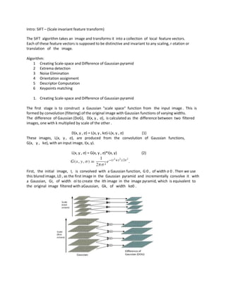
1. Intro: SIFT – (Scale invariant feature transform)
The SIFT algorithm takes an image and transforms it into a collection of local feature vectors.
Each of these feature vectors is supposed to be distinctive and invariant to any scaling, r otation or
translation of the image.
Algorithm:
1 Creating Scale-space and Difference of Gaussian pyramid
2 Extrema detection
3 Noise Elimination
4 Orientation assignment
5 Descriptor Computation
6 Keypoints matching
1. Creating Scale-space and Difference of Gaussian pyramid
The first stage is to construct a Gaussian "scale space" function from the input image . This is
formed by convolution (filtering) of the original image with Gaussian functions of varying widths.
The difference of Gaussian (DoG), D(x, y , σ), is calculated as the difference between two filtered
images, one with k multiplied by scale of the other .
D(x, y , σ) = L(x, y , kσ)-L(x, y , σ)
(1)
These images, L(x, y , σ), are produced from the convolution of Gaussian functions,
G(x, y , kσ), with an input image, I(x, y).
L(x, y , σ) = G(x, y , σ)*I(x, y)
(2)
First, the initial image, I, is convolved with a Gaussian function, G 0 , of width σ 0 . Then we use
this blured image, L0 , as the first image in the Gaussian pyramid and incrementally convolve it with
a Gaussian, Gi, of width σi to create the ith image in the image pyramid, which is equivalent to
the original image filtered with aGaussian, Gk, of width kσ0 .

2. 2. Extrema detection
This stage is to find the extrema points in the DOG pyramid. T o detect the local
maxima and minima of D(x, y , σ), each point is compared with the pixels of all its 26
neighbours . If this value is the minimum or maximum this point is an extrema.
3. Noise Elimination
This stage attempts to eliminate some points from the candidate list of keypoints by
finding those that have low contrast or are poorly localised on an edge.[1]. The value of the
keypoint in the DoG pyramid at the extrema is given by:
If the function value at z is below a threshold value this point is excluded.
T o eliminate poorly localized extrema we use the fact that in these cases there is a
large principle curvature across the edge but a small curvature in the perpendicular
direction in the difference of Gaussian function. A 2x2 Hessian matrix, H, computed at the
location and scale of the keypoint is used to find the curvature. With these fomulas,
the ratio of principal curvature can be checked efficiently .
Tr (H) = Dxx + Dyy
Det(H) = DxxDyy - (Dxy )2
R=Tr(H)^2/Det(H)
Where r= ratio between small and large Eigen value.
So if inequality fails, the key point is removed from the candidate list.

3. 4. Orientation assignment
This step aims to assign a consistent orientation to the keypoints based on local image
properties. An orientation histogram is formed from the gradient orientations of sample points within a
region around the keypoint . A 16x16 square is chosen in this implementation. The
orientation histogram has 36 bins covering the 360 degree range of orientations. The
gradient magnitude, m(x, y), and orientation, θ(x, y), is precomputed using pixel differences:
Each sample is weighted by its gradient magnitude and by a Gaussian-weighted circular window
with a σ that is 1.5 times that of the scale of the keypoint.
5. Descriptor Computation
In this stage, a descriptor is computed for the local image region that is as distinctive as possible at
each candidate keypoint. The image gradient magnitudes and orientations are sampled around the
keypoint location. These values are illustrated with small arrows at each sample location
on the first image of Figures. A Gaussian weighting function with σ related to the scale of the keypoint
is used to assign a weight to the magnitude.We use a σ equal to one half the width of the descriptor
window in this implementation. In order to achieve orientation invariance, the coordinates of
the descriptor and the gradient orientations are rotated relative to the keypoint orientation. This
process is indicated in Figure 5. In our implementation, a 16x16 sample array is computed and a
histogram with 8 bins is used. So a descriptor contains 16x16x8 elements in total. This vector is then
normalized to unit length in order to enhance invariance to affine changes in illumination.

4. 6. Keypoints matching
Knowing the keypoints and descriptors using Euclidean distance ,each keypoint in the original
image (model image) is compared to every keypoints in the transformed image using the
descriptors computed in the previous stage.
The descriptors of the two respective, keypoints must be closest. Then match is found.