SlideShare a Scribd company logo
1 of 76
Download to read offline
Naval Postgraduate School                                 Distance Learning


                                Antennas & Propagation

                                    LECTURE NOTES
                                      VOLUME II

 BASIC ANTENNA PARAMETERS AND WIRE
             ANTENNAS

                                by Professor David Jenn


                            r                λ
                            E

                       r                                     ANTENNA
                       H
                   ˆ
                   k
              PROPAGATION
               DIRECTION


                                                                              (ver 1.3)
Naval Postgraduate School                Antennas & Propagation                      Distance Learning


                   Antennas: Introductory Comments

      Classification of antennas by size:

      Let l be the antenna dimension:

             1. electrically small, l << λ : primarily used at low frequencies where the wavelength
                is long
             2. resonant antennas, l ≈ λ / 2: most efficient; examples are slots, dipoles, patches
             3. electrically large, l >> λ : can be composed of many individual resonant
                antennas; good for radar applications (high gain, narrow beam, low sidelobes)

      Classification of antennas by type:

             1. reflectors
             2. lenses
             3. arrays

      Other designations: wire antennas, aperture antennas, broadband antennas


                                                                                                         1
Naval Postgraduate School                                   Antennas & Propagation                                                         Distance Learning


                                  Radiation Integrals (1)
     Consider a perfect electric conductor (PEC) with an electric surface current flowing on S.
     In the case where the conductor is part of an antenna (a dipole), the current may be caused
     by an applied voltage, or by an incident field from another source (a reflector). The
     observation point is denoted by P and is given in terms of unprimed coordinate variables.
     Quantities associated with source points are designated by primes. We can use any
     coordinate system that is convenient for the particular problem at hand.
                                                                   OBSERVATION
                                            z                         POINT
                                                                     P ( x , y , z ) or P ( r ,θ ,φ )
                                                r
                                                r
                                                         r r r
                                                         R = r − r′                 r
                                   O                                             R= R =          ( x − x ′)2 + ( y − y ′)2 + ( z − z ′)2
                                       r
                                       r′                                 y
                                                    r
                            x
                                            S       J s ( x′, y ′, z ′)
                                    PEC WITH
                                SURFACE CURRENT

     The medium is almost always free space ( µo , ε o ), but we continue to use ( µ, ε ) to cover
     more general problems. If the currents are known, then the field due to the currents can be
     determined by integration over the surface.
                                                                                                                                                           2
Naval Postgraduate School                   Antennas & Propagation                             Distance Learning


                              Radiation Integrals (2)
      The vector wave equation for the electric field can be obtained by taking the curl of
      Maxwell’s first equation:
                                                r       r        r
                                        ∇ × ∇ × E = k 2 E − jωµJ s
                      r                                                 r r
      A solution for E in terms of the magnetic vector potential A(r ) is given by
                                                             r r
                                 r r           r r ∇ (∇ • A( r ) )
                                 E ( r ) = − jωA( r ) +                  (1)
                                                          jωµε
                                                                            r
              r                                             r r       µ     J s − jkR
      where (r ) is a shorthand notation for (x,y,z) and A( r ) =
                                                                     4π S∫∫ R e ds′
      We are particularly interested in the                           z                OBSERVATION
      case were the observation point is in the                                             POINT
      far zone of the antenna ( P → ∞ ). As P                               r
                                         r      r                           r
      recedes to infinity, the vectors r and R
                                                              r                       r r        r
      become parallel.                                        r′ • r
                                                                   ˆ                  R ≈ r − r (r ′ • r )
                                                                                              ˆ        ˆ

                                                                         r                    y
                                                                         r′
                                                               x

                                                                                                                   3
Naval Postgraduate School                      Antennas & Propagation                                Distance Learning


                                 Radiation Integrals (3)
                                   r r
      In the expression for A(r ) we use the approximation 1 / R ≈ 1 / r in the denominator and
          r        r     r
      r • R ≈ r • [r − r(r ′ • r )] in the exponent. Equation (2) becomes
       ˆ      ˆ        ˆ       ˆ
                      r r       µ     r − jk r •[r − r ( r ′• r )]
                                                 r       r               µ − jkr r jk (r ′• r )
                                                                                         r
                      A( r ) ≈     ∫∫ J s e                       ds′ =         ∫∫ J s e       ds′
                                             ˆ       ˆ        ˆ                             ˆ
                                                                            e
                               4πr S                                    4πr     S

      When this is inserted into equation (1), the del operations on the second term lead to 1 / r 2
                                                                           r
      and 1 / r 3 terms, which can be neglected in comparison to the − jωA term, which depends
      only on 1 / r . Therefore, in the far field,
            r r − jωµ − jkr r jk ( r ′• r )
            E (r ) ≈       ∫∫ J s e        ds′
                                    r ˆ
                         e                                 (discard the E r component)                 (3)
                     4πr   S

      Explicitly removing the r component gives,
                                  r r − jkη − jkr r           r                  r
                                                  ∫∫ [J s − r(J s • rˆ ) ]e
                                                                            jk ( r ′• r )
                                  E (r ) ≈      e           ˆ                         ˆ
                                                                                         ds′
                                           4π r   S

      The radial component of current does not contribute to the field in the far zone.
                                                                                                                         4
Naval Postgraduate School                Antennas & Propagation                         Distance Learning


                            Radiation Integrals (4)
                                                                                     r e − jkr
     Notice that the fields have a spherical wave behavior in the far zone: E ~                . The
                                                                                          r        r
     spherical components of the field can be found by the appropriate dot products with E .        r
     More general forms of the radiation integrals that include magnetic surface currents ( J ms )
     are:
                                                                 r
                                        − jkη − jkr  r ˆ J ms • φ  j k r ′⋅ r
                                                                     ˆ     r
                      Eθ ( r, θ , φ ) =            ∫∫  J s •θ +                ds′
                                                                              ˆ
                                         4π r
                                              e
                                                                   η   e
                                                   S 
                                                                 r
                                        − jkη − jkr  r ˆ J ms • θˆ  j k r′⋅r
                                                                           r
                      Eφ ( r, θ , φ ) =            ∫∫  J s •φ −                ds ′
                                                                              ˆ
                                         4π r
                                              e
                                                                   η   e
                                                   S 

      The radiation integrals apply to an unbounded medium. For antenna problems
                               the following process is used:
            1. find the current on the antenna surface, S,
            2. remove the antenna materials and assume that the currents are suspended
               in the unbounded medium, and
            3. apply the radiation integrals.
                                                                                                        5
Naval Postgraduate School                           Antennas & Propagation                         Distance Learning


                                          Hertzian Dipole (1)
      Perhaps the simplest application of the radiation integral is the calculation of the fields of
      an infinitesimally short dipole (also called a Hertzian dipole). Note that the criterion for
      short means much less than a wavelength, which is not necessarily physically short.
                            z                                       • For a thin dipole (radius, a << λ ) the
                                                                      surface current distribution is independent
                                                                      of φ ′ . The current crossing a ring around
                                     2a                                                    r
                                                                      the antenna is I = J s 2π a
                                                                                          {
                                                                                         A/m
               l                                                    • For a thin short dipole ( l << λ ) we assume
                                                                      that the current is constant and flows along
                                z′ r                                  the center of the wire; it is a filament of
                                  J s ( ρ ′, φ ′, z ′) = J o z
                                                             ˆ        zero diameter. The two-dimensional
                            φ′                           y            integral over S becomes a one-dimensional
                               ρ′ = a                                 integral over the length,
           x                                                                        r                    r
                                                                                 ∫∫ J s ds ′ → 2πa ∫ I d l′
                                                                                S              L


                                                                                                                       6
Naval Postgraduate School                      Antennas & Propagation                                     Distance Learning


                                  Hertzian Dipole (2)
            r                                                             r
     Using r ′ = zz ′ and r = x sin θ cosφ + y sin θ sin φ + z cosθ gives r ′ • r = z ′ cos θ . The
                 ˆ        ˆ ˆ                ˆ               ˆ                  ˆ
     radiation integral for the electric field becomes
                 r                − jkη − jkr l jk (r ′• r )         − jkηI z − jkr l
                                                                            ˆ                ′
                 E ( r, θ , φ ) ≈      e      ∫ Ie  r ˆ
                                                             zdrz′ =
                                                             {
                                                             ˆ                e     ∫   e jkz cosθ dz ′
                                   4πr        0               dl ′     4πr          0

     However, because l is very short, kz ′ → 0 and e jkz ′ cosθ              ≈ 1.   Therefore,
                          r                − jkηI z − jkr l
                          E ( r, θ , φ ) ≈
                                                  ˆ
                                                    e     ∫ (1) dz ′ = − jkηIl z e − jkr
                                                                               ˆ
                                             4πr          0               4πr
     leading to the spherical field components                             z

                       r
                   ˆ • E ≈ − jkηIlθ • z e − jkr
                                    ˆ ˆ
             Eθ = θ
                               4πr                                            l
                   jkηIl sin θ − jkr                                                   z′
                =             e
                       4πr
                       r                                                  x                 y
             Eφ = φˆ•E = 0
                                                                         SHORT CURRENT
                                                                           FILAMENT

                                                                                                                          7
Naval Postgraduate School                   Antennas & Propagation                   Distance Learning


                                   Hertzian Dipole (3)
     Note that the electric field has only a 1/r dependence. The absence of higher order terms
     is due to the fact that the dipole is infinitesimal, and therefore r ff → 0 . The field is a
     spherical wave and hence the TEM relationship can be used to find the magnetic field
     intensity
                               r k × E r × Eθ θˆ
                                                        ˆ jkIl sin θ e − jkr
                                    ˆ ˆ ˆ
                               H=         =          =φ
                                     η          η            4πr
     The time-averaged Poynting vector is
                             r   1 ˆ r* 1
                                     {      }        {
                            Wav = ℜ E × H = ℜ Eθ Hφ r =
                                                  *
                                                    ˆ         }
                                                        ηk 2 I 2 l2 sin 2 θ
                                                                            r
                                                                            ˆ
                                 2         2                 32π r2 2

     The power flow is outward from the source, as expected for a spherical wave. The
     average power flowing through the surface of a sphere of radius r surrounding the source
     is
                2π π r
                                  ηk 2 I 2 l2 2π π 2                           ηk 2 I 2 l2
          Prad = ∫ ∫ Wav • n ds =
                           ˆ                   ∫ ∫ sin θ r • rˆ r sin θ dθ dφ = 12π W
                                                         ˆ       2
                                   32π 2r 2 0 0
                 0 0                          14444 244444
                                                         4                 3
                                                                = 8π / 3

                                                                                                     8
Naval Postgraduate School                  Antennas & Propagation                 Distance Learning


                            Solid Angles and Steradians
      Plane angles: s = Rθ , if s = R then θ = 1 radian
                                                                 ARC LENGTH
                                      R                             s
                                      θ


      Solid angles: Ω = A / R2 , if A = R 2 , then Ω = 1 steradian


                              Ω = A / R2                                SURFACE
                                                                        AREA
                                                             R           A


                                                                                                      9
Naval Postgraduate School                            Antennas & Propagation                    Distance Learning


                                Directivity and Gain (1)
     The radiation intensity is defined as
                                            dPrad          r     2 r
                               U (θ , φ ) =       = r r • Wav = r Wav
                                                     2
                                                       ˆ
                                             dΩ
     and has units of Watts/steradian (W/sr). The directivity function or directive gain is
     defined as
                                                                                        r
                         power radiated per unit solid angle     dP / dΩ           r 2 Wav
         D(θ , φ ) =                                            = rad         = 4π
                     average power radiated per unit solid angle Prad /( 4π )        Prad
     For the Hertzian dipole,
                                                                  2 ηk I l sin θ
                                                                      2   2
                                                                          2   2
                                               r              r
                                             2
                                             r Wav                     32π 2 r 2    3
                            D(θ , φ ) = 4π             = 4π                        = sin 2 θ
                                                                    ηk 2 I l 2
                                              Prad                            2     2
                                                                       12π
     The directivity is the maximum value of the directive gain
                                                                                    3
                                         Do = Dmax (θ ,φ ) = D (θ max ,φ max ) =
                                                                                    2
                                                                                                              10
Naval Postgraduate School                             Antennas & Propagation                                  Distance Learning


                             Dipole Polar Radiation Plots
      Half of the radiation pattern of the dipole is plotted below for a fixed value of φ . The half-
      power beamwidth (HPBW) is the angular width between the half power points (1/ 2
      below the maximum on the voltage plot, or –3dB below the maximum on the decibel plot).
                             FIELD (VOLTAGE) PLOT                              DECIBEL PLOT
                                        90     1.5                                   90 10
                                  120                60                        120             60
                                                                                       0
                                              1
                            150                            30          150             -10          30
                                              0.5
                                                                                       -20

                       180                                       θ
                                                                 0   180                            θ     0


                            210                            330         210                          330


                                  240                300                       240            300
                                        270                                          270

      The half power beamwidth of the Hertzian dipole, θ B :

           Enorm ~ sin θ           ⇒ sin (θ HP ) = 0.707 ⇒ θ HP = 45o                        ⇒ θ B = 2θ HP = 90o


                                                                                                                              11
Naval Postgraduate School              Antennas & Propagation                      Distance Learning


                            Dipole Radiation Pattern
      Radiation pattern of a Hertzian dipole aligned with the z axis. Dn is the normalized
      directivity. The directivity value is proportional to the distance from the center.


                                                                                                   12
Naval Postgraduate School                Antennas & Propagation                        Distance Learning


                            Directivity and Gain (2)
     Another formula for directive gain is
                                               4π r              2
                                    D(θ ,φ ) =    Enorm (θ , φ )
                                               ΩA
     where Ω A is the beam solid angle
                                      2π π   r              2
                               ΩA =   ∫∫     E norm (θ , φ ) sin θ dθ dφ
                                      0 0
         r
     and E norm (θ ,φ ) is the normalized magnitude of the electric field pattern (i.e., the
     normalized radiation pattern)
                                                       r
                                    r                  E ( r ,θ , φ )
                                   E norm (θ , φ ) = r
                                                     Emax ( r, θ , φ )

     Note that both the numerator and denominator have the same 1/r dependence, and hence
     the ratio is independent of r. This approach is often more convenient because most of our
     calculations will be conducted directly with the electric field. Normalization removes all
     of the cumbersome constants.
                                                                                                      13
Naval Postgraduate School                      Antennas & Propagation                       Distance Learning


                               Directivity and Gain (3)
      As an illustration, we re-compute the directivity of a Hertzian dipole. Noting that the
      maximum magnitude of the electric field is occurs when θ = π / 2 , the normalized electric
      field intensity is simply         r
                                       E norm (θ ,φ ) = sin θ
      The beam solid angle is
                                              2π π   r              2
                                     ΩA =     ∫∫     E norm (θ , φ ) sin θ dθ dφ
                                              0 0
                                                π
                                                               8π
                                           = 2π ∫ sin 3 θ dθ =
                                                                3
                                                14 4
                                                0    2 3
                                                      =4 / 3

      and from the definition of directivity,
                                         4π r             2   4π            2    3
                            D(θ ,φ ) =      Enorm (θ , φ ) =        sin θ       = sin 2 θ
                                         ΩA                  8π / 3              2
      which agrees with the previous result.

                                                                                                            14
Naval Postgraduate School                                        Antennas & Propagation                                Distance Learning


                                                                  Example
      Find the directivity of an antenna whose far-electric field is given by
                          90            10
                    120                      60
                                    8

                                    6
                                                                                      10e − jkr
                                                                                                 cos θ , 0o ≤ θ ≤ 90o
              150                                  30


                                                                                      
                                4


                                                                                       r
                                2

            180                                          0
                                                                    Eθ ( r, θ , φ ) =  − jkr
                                                                                      e      cos θ , 90o ≤ θ ≤ 180 o
                                                                                       r
                                                                                      
              210                                  330


                    240                      300


                                                                                                 r
                          270


      The maximum electric field occurs when cosθ = 1 →                                          Emax = 10 / r . The normalized
      electric field intensity is
                                                  cos θ ,
                                                             0o ≤ θ ≤ 90o
                              Eθ norm (θ , φ ) = 
                                                 0.1 cosθ , 90o ≤ θ ≤ 180o
                                                 
      which gives a beam solid angle of
                                2π π / 2                                       2π π
                                                                                                                 2π
                    ΩA =            ∫ ∫            cos θ sin θ dθ dφ + 0.01 ∫       ∫     cos2 θ sin θ dθ dφ =
                                                             2
                                                                                                                    (1.1)
                                    0          0                                0 π /2
                                                                                                                  3

      and a directivity of Do = 5.45 = 7.37 dB.
                                                                                                                                       15
Naval Postgraduate School                          Antennas & Propagation                         Distance Learning


            Beam Solid Angle and Radiated Power
      In the far field the radiated power is

                     1
                         2π π      r r
                                  E × H *  • r ds      1
                                                             2π π   r2 2
            Prad   =
                     2   ∫∫     ℜ
                                1 4 44
                                 4 2 3
                                            ˆ        =
                                                        2η     ∫∫   E r sin θ dθ dφ   ⇒   Frad = 2ηPrad
                         0 0        r2
                                    E /η
                                                             144424443
                                                             0 0 4   4
                                                                         ≡ Frad
      From the definition of beam solid angle
                            2π π    r              2
                   ΩA =     ∫∫      E norm (θ , φ ) sin θ dθ dφ
                            0 0
                                   1       2π π   r2 2                           r    2
                                2 2 ∫ ∫
                         = r                      E r sin θ dθ dφ = ⇒ Frad = Ω A E max r 2
                           E max r 1444 24444
                                    0 0 4   3
                                                      ≡ Frad
      Equate the expressions for Frad
                                                                 r    2
                                                             Ω A E max r 2
                                                   Prad =
                                                                    2η


                                                                                                                  16
Naval Postgraduate School                  Antennas & Propagation                               Distance Learning


                              Gain vs. Directivity (1)

      Directivity is defined with respect to the radiated power, Prad . This could be less than the
      power into the antenna if the antenna has losses. The gain is referenced to the power into
      the antenna, Pin .
                                                       ANTENNA
                                                  I
                                    Pinc                      Rl
                                           Pref        Pin          Ra

      Define the following:
             Pinc = power incident on the antenna terminals
             Pref = power reflected at the antenna input
             Pin = power into the antenna
                                                                                       1    2
             Ploss = power loss in the antenna (dissipated in resistor Rl , Ploss =        I Rl )
                                                                                       2
                                                                         1    2
             Prad = power radiated (delivered to resistor Ra , Prad =        I Ra , Ra is the radiation
                                                                         2
                      resistance)
      The antenna efficiency, e, is Prad = ePin where 0 ≤ e ≤ 1 .

                                                                                                                17
Naval Postgraduate School                      Antennas & Propagation                              Distance Learning


                             Gain vs. Directivity (2)
      Gain is defined as
                                           dPrad / dΩ     dP / dΩ
                            G (θ , φ ) =              = 4π rad      = eD(θ , φ )
                                           Pin /(4π )      Prad / e

      Most often the use of the term gain refers to the maximum value of G(θ , φ ) .

      Example: The antenna input resistance is 50 ohms, of which 40 ohms is radiation
      resistance and 10 ohms is ohmic loss. The input current is 0.1 A and the directivity of the
      antenna is 2.

                                   1       2       1        2
      The input power is Pin =         I Rin =         0.1 ( 50) = 0.25 W
                                   2               2
                                                                    1    2     1   2
      The power dissipated in the antenna is Ploss =                    I Rl = 0.1 (10) = 0.05 W
                                                                    2          2
                                                        1       2        1    2
      The power radiated into space is Prad =               I Ra = 0.1 (40 ) = 0.2 W
                                                        2                2

      If the directivity is Do = 2 then the gain is G = eD =  rad  D = 
                                                               P            0 .2 
                                                                              ( 2) = 1.6
                                                              Pin       0.25 


                                                                                                                   18
Naval Postgraduate School               Antennas & Propagation                         Distance Learning


             Azimuth/Elevation Coordinate System
      Radars frequently use the azimuth/elevation coordinate system: (Az,El) or (α ,γ ) or
      (θ e , φ a ). The antenna is located at the origin of the coordinate system; the earth's surface
      lies in the x-y plane. Azimuth is generally measured clockwise from a reference (like a
      compass) but the spherical system azimuth angle φ is measured counterclockwise from the
      x axis. Therefore α = 360 − φ and γ = 90 − θ degrees.
                                       ZENITH

                                        z


                                                                  CONSTANT
                                                                  ELEVATION


                                                          P
                                            θ       r
                                                γ                    y
                                            φ
                            α
                            x                           HORIZON

                                                                                                       19
Naval Postgraduate School              Antennas & Propagation                        Distance Learning


               Approximate Directivity Formula (1)
      Assume the antenna radiation pattern is a “pencil beam” on the horizon. The pattern is
      constant inside of the elevation and azimuth half power beamwidths (θ e , φa ) respectively:
                                                   z
                                                       θ =0


                                                                         y


                                                   θe                x
                                                              φa   φ =0
                                                                   θ =π /2


                                                                                                     20
Naval Postgraduate School                     Antennas & Propagation                              Distance Learning


               Approximate Directivity Formula (2)
      Approximate antenna pattern

         r             Eoe − jkr
                      
         E (θ , φ ) =  r         θˆ, (π / 2 − θ e / 2 ) ≤ θ ≤ (π / 2 + θ e / 2 ) and − φa / 2 ≤ φ ≤ φa / 2
                      0,
                                     else
      The beam solid angle is
                                             π θe     φa
                                              +
                                             2 2       2
                                     ΩA =       ∫      ∫   sin θ dθ dφ
                                                           {
                                             π θe
                                              −
                                                      φ
                                                     − a
                                                            ≈1
                                             2 2       2
                                          = φa [sin (θ e / 2 ) − sin (− θ e / 2 )]
                                          ≈ φa [θ e / 2 − ( −θ e / 2 )] = φaθ e
                                                                  4π     4π
      This leads to an approximation for the directivity of Do =      =       . Note that the
                                                                 Ω A θ eφa
      angles are in radians. This formula is often used to estimate the directivity of an omni-
      directional antenna with negligible sidelobes.


                                                                                                                  21
Naval Postgraduate School                     Antennas & Propagation                         Distance Learning


                            Thin Wire Antennas (1)
     Thin wire antennas satisfy the condition a << λ . If the length of the wire (l ) is an integer
     multiple of a half wavelength, we can make an “educated guess” at the current based on
     an open circuited two-wire transmission line
                                              FEED POINTS

                                                            λ /4
                                                                                  λ/2
                               z
                                                              OPEN
                            I(z)                             CIRCUIT

     For other multiples of a half wavelength the current distribution has the following features
                                                               FEED POINT
                                                               LOCATED AT
                                                                MAXIMUM


                                   l = λ /2           l=λ
                                                                            CURRENT GOES
                                                                            TO ZERO AT END


                                               l = 3λ / 2


                                                                                                            22
Naval Postgraduate School                     Antennas & Propagation                          Distance Learning


                              Thin Wire Antennas (2)
      On a half-wave dipole the current can be approximated by
                                      I ( z ) = I o cos( kz) for − λ / 4 < z < λ / 4
      Using this current in the radiation integral
                            r                − jkη − jkr λ / 4
                            E ( r ,θ , φ ) =      e     z ∫ I o cos( kz′) e jkz ′ cosθ dz ′
                                                        ˆ
                                              4πr         −λ / 4
                                       − jkηI o − jkr λ / 4
                                    =              e      z ∫ cos( kz′) e jkz ′ cosθ dz ′
                                                          ˆ
                                          4πr               −λ / 4
      From a table of integrals we find that
                                                     Az ′
                                                             6 74
                                                             4= 0 8        6= ±4
                                                                            4 187
                                                   e [ A cos( Bz′) + B sin ( Bz′)]
                         ∫ cos( Bz ′) e Az ′dz ′ =
                                                                 A2 + B 2
      where A = jk cos θ and B = k , so that A2 + B 2 = − k 2 cos 2 θ + k 2 = k 2 sin 2 θ . The θ
      component requires the dot product z • θˆ = − sin θ .
                                           ˆ


                                                                                                              23
Naval Postgraduate School                  Antennas & Propagation                            Distance Learning


                            Thin Wire Antennas (3)
     Evaluating the limits gives
                                              π
                                       2 cos cosθ 
                                                  
                                    64444 4 74444 8
                                                    4                                    π      
                                              2
                                                                                       cos cos θ 
             jkηI o − jkr       k[e jπ cosθ / 2 − ( −1)e − jπ cosθ / 2 ] jηI o − jkr      2      
        Eθ =       e      sin θ                                         =      e
              4π r                            k sin θ
                                                2    2                    2π r             sin θ
     The magnetic field intensity in the far field is
                                   r                      π      
                                                       cos cos θ 
                            r k×E
                               ˆ                          2      φ
                            H=          ˆE    jI
                                     = φ θ = o e − jkr              ˆ
                                 η       H φ 2πr           sin θ

     The directivity is computed from the beam solid angle, which requires the normalized
     electric field intensity

                                  r     2
                                  E norm =
                                                 Eθ
                                                      2
                                                              =
                                                                    (π
                                                                  cos cos θ
                                                                     2
                                                                              )   2


                                              Eθ max
                                                          2         sin θ


                                                                                                            24
Naval Postgraduate School                            Antennas & Propagation                                        Distance Learning


                                Thin Wire Antennas (4)
                      π                                             π
                            cos (π cos θ / 2 )
                               2
                                                                         cos 2 (π cos θ / 2 )
         Ω A = 2π
                      ∫            sin θ
                                     2
                                                 sin θ dθ = 2π
                                                                    ∫             sin θ
                                                                                     2
                                                                                                    dθ = ( 2π )(1.218)
                      0                                             1444 2444 3
                                                                    0  4     4
                                                                     Integrate numericall y
     The directive gain is

                D=
                   4π r             2
                      Enorm (θ , φ ) =
                                             4π      cos 2 cos θ
                                                           2     = 1.64
                                                                             (π
                                                                        cos 2 cos θ
                                                                              2
                                                                                      )                  (π
                                                                                                                   )
                   ΩA                  ( 2π )(1.218)    sin 2 θ            sin 2 θ
     The radiated power is
                                           2 2
                            Ω A Eθ max r                                 2
                                                     2π (1.218)η 2 I o r 2                      2       1 2
                  Prad =                         =                                = 36.57 I o       ≡     I o Ra
                                    2η                    2η ( 2π r) 2                                  2
     where Ra is the radiation resistance of the dipole. The radiated power can be viewed as
     the power delivered to resistor that represents “free space.” For the half-wave dipole the
     radiation resistance is
                                   2P
                             Ra = rad = ( 2 )(36.57 ) = 73.13 ohms
                                       2
                                    Io
                                                                                                                                  25
Naval Postgraduate School                                          Antennas & Propagation                 Distance Learning


                               Numerical Integration (1)
     The rectangular rule is a simple way of evaluating an integral numerically. The area under
     the curve of f ( x) is approximated by a sum of rectangular areas of width ∆ and height
                                     ∆
      f ( xn ) , where xn =              + ( n − 1) + a is the center of the interval nth interval. Therefore, if
                                     2
     all of the rectangles are of equal width
                                                               b                   b
                                                               ∫ f ( x ) dx ≈ ∆ ∑ f ( xn )
                                                               a                   a
     Clearly the approximation can be made as close to the exact value as desired by reducing
     the width of the triangles as necessary. However, to keep computation time to a minimum,
     only the smallest number of rectangles that provides a converged solution should be used.

                                                       2             3
                                              1                            4
                            f ( x)
                                                                                                  N
                                              ∆
                                                                                        L

                                              •            •                                 •
                                                                                                      x
                                          a                                                       b
                                                  x1       x2                                xN


                                                                                                                         26
Naval Postgraduate School                         Antennas & Propagation                Distance Learning


                               Numerical Integration (2)
                                                          π
                                                               cos 2 (π cosθ / 2 )
     Example: Matlab programs to integrate
                                                           ∫
                                                           0
                                                                      sin θ
                                                                                   dθ

     Sample Matlab code for the rectangular rule
                            % integrate dipole pattern using the rectangular rule
                            clear
                            rad=pi/180;
                            % avoid 0 by changing the limits slightly
                            a=.001; b=pi-.001;
                            N=5
                            delta=(b-a)/N;
                            sum=0;
                            for n=1:N
                                   theta=delta/2+(n-1)*delta;
                                   sum=sum+cos(pi*cos(theta)/2)^2/sin(theta);
                            end
                            I=sum*delta
     Convergence: N=5, 1.2175; N=10, 1.2187; N=50, 1.2188. Sample Matlab code using the
     quad8 function
                            % integrate to find half wave dipole solid angle
                            clear
                            I=quad8('cint',0.0001,pi-.0001,.00001);
                            disp(['cint integral, I: ',num2str(I)])

                            function P=cint(T)
                            % function to be integrated
                            P=(cos(pi*cos(T)/2).^2)./sin(T);


                                                                                                       27
Naval Postgraduate School                        Antennas & Propagation                                Distance Learning


                      Thin Wires of Arbitrary Length
     For a thin-wire antenna of length l along the z axis, the electric field intensity is
                                              kl               kl  
                                              cos cosθ  − cos  
                                  jηI − jkr   2               2
                           Eθ =      e                                 
                                 2πr                  sin θ            
                                            
                                                                       
                                                                        
     Example: l = 1.5λ (left: voltage plot; right: decibel plot)
                                  90 2                                          9010
                            120             60                            120           60
                                                                                  0

                     150                1           30            150             -10         30
                                                                                  -20

                   180                                   0     180                                 0


                     210                            330           210                         330

                            240             300                           240           300
                                  270                                           270


                                                                                                                      28
Naval Postgraduate School               Antennas & Propagation                      Distance Learning


           Feeding and Tuning Wire Antennas (1)
     When an antenna terminates a transmission line, as shown below, the antenna impedance
     ( Z a ) should be matched to the transmission line impedance ( Zo ) to maximize the power
     delivered to the antenna

                                                             Za − Zo            1+ Γ
                            Zo   Za                    Γ=            and VSWR =
                                                             Za + Zo            1− Γ


     The antenna’s input impedance is generally a complex quantity, Z a = ( Ra + Rl ) + jX a .
     The approach for matching the antenna and increasing its efficiency is

            1. minimize the ohmic loss, Rl → 0
            2. “tune out” the reactance by adjusting the antenna geometry or adding lumped
               elements, X a → 0 (resonance occurs when Z a is real)
            3. match the radiation resistance to the characteristic impedance of the line by
               adjusting the antenna parameters or using a transformer section, Ra → Zo


                                                                                                   29
Naval Postgraduate School               Antennas & Propagation                       Distance Learning


            Feeding and Tuning Wire Antennas (2)
      Example: A half-wave dipole is fed by a 50 ohm line

                                       Z a − Z o 73 − 50
                                    Γ=           =        = 0.1870
                                       Z a + Z o 73 + 50
                                                1+ Γ
                                      VSWR =         = 1.46
                                                1− Γ

      The loss due to reflection at the antenna terminals is

                                           2          2
                                       τ       = 1 − Γ = 0.965
                                      10 log τ ( ) = −0.155 dB
                                                 2


      which is stated as “0.155 dB of reflection loss” (the negative sign is implied by using the
      word “loss”).


                                                                                                     30
Naval Postgraduate School                   Antennas & Propagation                         Distance Learning


           Feeding and Tuning Wire Antennas (3)
     The antenna impedance is affected by
          1. length
          2. thickness
          3. shape
          4. feed point (location and method of feeding)
          5. end loading
     Although all of these parameters affect both the real and imaginary parts of Z a , they are
     generally used to remove the reactive part. The remaining real part can be matched using
     a transformer section.
     Another problem is encountered when matching a balanced radiating structure like a
     dipole to an unbalanced transmission line structure like a coax.
                              UNBALANCED FEED                        BALANCED FEED


                                    COAX
                                                                       TWO-WIRE LINE
                                                                +
                          +
                                                  λ /2     Vg                            λ /2
                     Vg                                         −
                          −
                                       DIPOLE                                   DIPOLE


                                                                                                          31
Naval Postgraduate School                 Antennas & Propagation                   Distance Learning


           Feeding and Tuning Wire Antennas (4)
     If the two structures are not balanced, a return current can flow on the outside of the
     coaxial cable. These currents will radiate and modify the pattern of the antenna. The
     unbalanced currents can be eliminated using a balun (balanced-to-unbalanced transformer)
                            UNBALANCED FEED                    BALANCED FEED

                                                  I (z )
                                 a b                               a b
                                  ..                                ..
                                       Va ≠ Vb                           Va = Vb


     Baluns frequently incorporate chokes, which are circuits designed to “choke off” current
     by presenting an open circuit to current waves.


                                                                                                  32
Naval Postgraduate School                  Antennas & Propagation                     Distance Learning


           Feeding and Tuning Wire Antennas (5)
     An example of a balun employing a choke is the sleeve or bazooka balun
                            I2             I1

                                                       HIGH IMPEDANCE (OPEN CIRCUIT)
                                                       PREVENTS CURRENT FROM FLOWING
                λ /4         ′
                            Zo
                                                       ON OUTSIDE
                                 I2   I1

                                                    SHORT CIRCUIT
                                 Zo


     The choke prevents current from flowing on the exterior of the coax. All current is
     confined to the inside of surfaces of the coax, and therefore the current flow in the two
     directions is equal (balanced) and does not radiate. The integrity of a short circuit is easier
     to control than that of an open circuit, thus short circuits are used whenever possible.
     Originally balun referred exclusively to these types of wire feeding circuits, but the term
     has evolved to refer to any feed point matching circuit.

                                                                                                     33
Naval Postgraduate School               Antennas & Propagation                             Distance Learning


            Calculation of Antenna Impedance (1)
     The antenna impedance must be matched to that of the feed line. The impedance of an
     antenna can be measured or computed. Usually measurements are more time consuming
     (and therefore expensive) relative to computer simulations. However, for a simulation to
     accurately include the effect of all of the antenna’s geometrical and electrical parameters
     on Z a , a fairly complicated analytical model must be used. The resulting equations must
     be solved numerically in most cases.
     One popular technique is the method of moments (MM) solution of an integral equation
     (IE) for the current.
                        z
                                                1. I (z ′) is the unknown current distribution on the
                            l/ 2                   wire
                                                2. Find the z component of the electric field in
                              2a                   terms of I (z ′) from the radiation integral
            +               b/ 2                3. Apply the boundary condition
           Vg           Eg
                −            −b / 2
                                                                              0, b /2 ≤ z ≤ l / 2
                                                                 Ez (ρ = a) = E , b /2 ≥ z
                                                                               g

                             −l /2                  in order to obtain an integral equation for I (z ′)


                                                                                                          34
Naval Postgraduate School                 Antennas & Propagation                       Distance Learning


              Calculation of Antenna Impedance (2)
      One special form of the integral equation for thin wires is Pocklington’s equation
                             2 ∂2  l / 2       e − jkR       0, b / 2 ≤ z ≤ l / 2
                             k + 2  ∫ I( z ′ )         dz′ = − jωεE , b / 2 ≥ z
                                ∂z  −l / 2      4πR                 g


      where R = a 2 + ( z − z ′) 2 . This is called an integral equation because the unknown
      quantity I (z ′) appears in the integrand.
      4. Solve the integral equation using the method of moments (MM). First approximate the
      current by a series with unknown expansion coefficients {I n }
                                                     N
                                           I( z ′ ) = ∑ InΦ n ( z ′ )
                                                    n=1

      The basis functions or expansion functions {Φ n } are known and selected to suit the
      particular problem. We would like to use as few basis functions as possible for
      computational efficiency, yet enough must be used to insure convergence.


                                                                                                       35
Naval Postgraduate School                          Antennas & Propagation                               Distance Learning


              Calculation of Antenna Impedance (3)
      Example: a step approximation to the current using a series of pulses. Each segment is
      called a subdomain. Problem: there will be discontinuities between steps.
                                                             I( z ′)
                                  CURRENT                                            STEP
                                                                                APPROXIMATION
                                       I 2 Φ2

                            I1Φ1                                                   IN Φ N
                                          ∆        L                      L
                                  •       •                       •               •           z′
                            −l    z1     z2              0                       zN   l
                            2                                                         2
      A better basis function is the overlapping piecewise sinusoid
                                                                 I( z′)
                                       CURRENT                                PIECEWISE
                                                                              SINUSOID
                                       I2 Φ2

                             I1Φ1                  L             ∆          L         I NΦN

                                    •         •                                     •
                                                                                                   z′
                                 −l z         z2             0                     zN     l
                                     1
                                 2                                                        2

                                                                                                                        36
Naval Postgraduate School               Antennas & Propagation                        Distance Learning


            Calculation of Antenna Impedance (4)
     A piecewise sinusoid extends over two segments (each of length ∆ ) and has a maximum at
     the point between the two segment
                                                               z′ − zn−1 , z ′ ≤ z ′ ≤ z ′
                                                                      ′
                                                                              n−1          n
                               Φ n(z′)                         z′ − zn−1
                                                                 n     ′
                                                              
                                                               zn+1 − z ′
                                                                 ′
                                                  Φ n (z ′) =             , zn ≤ z ′ ≤ zn+1
                                                                               ′         ′
                                                                z′ − zn  ′
                                            z′                 n+1
               zn − ∆       zn z n + ∆
                                                              0,            elsewhere
               ( = z n −1 )     ( = zn +1 )                   
                                                              

                                                                      Φn( z′ )
     Entire domain functions are also                                  Φ1
     possible. Each entire domain
     basis function extends over the                                                               z′
     entire wire. Examples are               −l                                  Φ2      l
                                                                 Φ3
     sinusoids.                              2                                           2


                                                                                                     37
Naval Postgraduate School                              Antennas & Propagation                        Distance Learning


            Calculation of Antenna Impedance (5)
     Solving the integral equation: (1) insert the series back into the integral equation
                   2 ∂2  l / 2  N                 e − jkR          0, b / 2 ≤ z ≤ l / 2
                   k + 2  ∫  ∑ InΦ n (z ′ )                dz′ = − jωεE , b / 2 ≥ z
                                                                     
                          ∂z  −l / 2  n=1         4πR                    g

     Note that the derivative is with respect to z (not z ′ ) and therefore the differential operates
     only on R . For convenience we define new functions f and g:
           N      l / 2  2 ∂2 
                                            e − jkR ( z, z′)  0,
                                                                                 b/ 2 ≤ z ≤ l/ 2
           ∑ I n  ∫  k + 2  Φ n ( z ′)
                                                           dz′ = 
                                                                      − jωεE g , b / 2 ≥ z
          n =1 − l / 2                    4πR ( ′) 
                  4444∂z 4 24444z, z44  4444 244444
                 1              4 4                  4 3            1           4             3
                                       ≡ f ( Φ n )→ f n ( z )                              ≡g
     Once Φ n is defined, the integral can be evaluated numerically. The result will still be a
     function of z, hence the notation f n (z ) .
     (2) Choose a set of N testing (or weighting) functions {Χ m }. Multiply both sides of the
     equation by each testing function and integrate over the domain of each function ∆ m to
     obtain N equations of the form

                            ∫ Χ m ( z )n∑1I n f n (z ) dz = ∫ Χ m (z ) g (z )dz ,
                                        N
                                                                                    m = 1,2,..., N
                                        =
                            ∆m                                  ∆m

                                                                                                                    38
Naval Postgraduate School                   Antennas & Propagation                    Distance Learning


            Calculation of Antenna Impedance (6)
     Interchange the summation and integration operations and define new impedance and
     voltage quantities
                           N                             
                                                         
                                  ∑   ∫                              ∫
                              I n  Χ m ( z) f mn ( z) dz  = Χ m ( z) g ( z)dz
                          n =1 ∆ m
                                   444 444  ∆ m44 44    
                                  1        2            3 1        2         3
                                         Z mn                     Vm
     This can be cast into the form of a matrix equation and solved using standard matrix
     methods
                            N
                            ∑ In Zmn = Vm   → [ Z][I ] = [V ] → [ I ] = [Z ]−1[V ]
                            n=1
     [Z ] is a square impedance matrix that depends only on the geometry and material
     characteristics of the dipole. Physically, it is a measure of the interaction between the
     currents on segments m and n. [V ] is the excitation vector. It depends on the field in the
     gap and the chosen basis functions. [I ] is the unknown current coefficient vector.
     After [I ] has been determined, the resulting current series can be inserted in the radiation
     integral, and the far fields computed by integration of the current.


                                                                                                     39
Naval Postgraduate School                Antennas & Propagation                 Distance Learning


                 Self-Impedance of a Wire Antenna
     The method of moments current allows calculation of the self impedance of the antenna by
     taking the ratio Zself = Vg / Io

                            RESISTANCE                            REACTANCE


                                                                                               40
Naval Postgraduate School                Antennas & Propagation                         Distance Learning


                  The Fourier Series Analog to MM
     The method of moments is a general solution method that is widely used in all of
     engineering. A Fourier series approximation to a periodic time function has the same
     solution process as the MM solution for current. Let f (t ) be the time waveform
                                         ao 2 ∞
                                 f (t) =   + ∑ [an cos(ω nt ) + bn sin (ω nt )]
                                         T T n =1
     For simplicity, assume that there is no DC component and that only cosines are necessary
     to represent f (t ) (true if the waveform has the right symmetry characteristics)
                                                      2 ∞
                                           f ( t ) = ∑ an cos(ωn t )
                                                     T n =1
     The constants are obtained by multiplying each side by the testing function cos(ω m t) and
     integrating over a period
                                                                                      0, m ≠ n
                                         2 T /2  ∞
                                                            (ω nt ) cos(ω mt ) dt = 
              T /2
                ∫ f ( t ) cos(ω mt )dt =     ∫  ∑ a cos                            
             −T / 2                      T −T / 2  n =1 n                          an , m = n
     This is analogous to MM when f ( t ) → I ( z ′) , a n → I n , Φ n → cos(ωn t ) , and
     Χ m → cos(ωm t ) . (Since f (t ) is not in an integral equation, a second variable t ′ is not
     required.) The selection of the testing functions to be the complex conjugates of the
     expansion functions is referred to as Galerkin’s method.
                                                                                                       41
Naval Postgraduate School                   Antennas & Propagation                        Distance Learning


                                      Reciprocity (1)
     When two antennas are in close proximity to each other, there is a strong interaction
     between them. The radiation from one affects the current distribution of the other, which
     in turn modifies the current distribution of the first one.
                                     ANTENNA 1                       ANTENNA 2
                                      (SOURCE)                       (RECEIVER)

                                             I1                      I2

                                 +
                            V1                                            Eg        V21
                                 −

                                     Z1                                        Z2

     Consider two situations (depicted on the following page) where the geometrical
     relationship between two antennas does not change.
     1. A voltage is applied to antenna 1 and the current induced at the terminals of antenna 2 is
        measured.
     2. The situation is reversed: a voltage is applied to antenna 2 and the current induced at the
        terminals of antenna 1 is measured.
                                                                                                         42
Naval Postgraduate School                      Antennas & Propagation                         Distance Learning


                                       Reciprocity (2)
      Case 1:
                                   ANTENNA 1
                                                                               I2

                                                                                    CURRENT
                                                                                     METER
                                   +
                             V1
                                                      ENERGY FLOW
                                   −
                                                                        ANTENNA 2


      Case 2:
                                   ANTENNA 1                               +
                                                                                     V2
                                                                               −


                              I1                        ENERGY FLOW

                                                                        ANTENNA 2
                            CURRENT
                             METER


                                                                                                              43
Naval Postgraduate School              Antennas & Propagation                      Distance Learning


                            Mutual Impedance (1)
     Define the mutual impedance or transfer impedance as
                                               V2            V
                                       Z12 =       and Z21 = 1
                                               I1            I2
     The first index on Z refers to the receiving antenna (observer) and the second index to the
     source antenna.
     Reciprocity Theorem: If the antennas and medium are linear, passive and isotropic, then
     the response of a system to a source is unchanged if the source and observer (measurer)
     are interchanged.
     With regard to mutual impedance:
         • This implies that Z21 = Z12
         • The receiving and transmitting patterns of an antenna are the same if it is
            constructed of linear, passive, and isotropic materials and devices.
     In general, the input impedance of antenna number n in the presence of other antennas is
     obtained by integrating the total field in the gap (gap width bn )
                                             Vn 1 r          r
                                       Zn =      = ∫ En • dl
                                             In In
                                                      bn

                                                                                                  44
Naval Postgraduate School                   Antennas & Propagation                     Distance Learning


                                 Mutual Impedance (2)
      r
     En is the total field in the gap of antenna n (due to its own voltage plus the incident fields
     from all other antennas).


                            Vn    En

                                       In


                                                                                                      45
Naval Postgraduate School             Antennas & Propagation                   Distance Learning


                            Mutual Impedance (3)
     If there are a total of N antennas
                                     r     r      r        r
                                     En = En1 + En2 + L + EnN
     Therefore,
                                             1      N r    r
                                             In ∫ m=1 nm
                                       Zn =         ∑ E • dln
                                               bn
     Define
                                                  r      r
                                      Vnm     = ∫ E nm• d ln
                                                bn
     The impedance becomes
                                    1 N         N V     N
                              Zn =      ∑ Vnm = ∑  nm =
                                                        ∑ Z nm
                                   I n m =23 m =1 I n m =1
                                       11         {
                                        ≡Vn           ≡ Z nm
     For example, the impedance of dipole n=1 is written explicitly as
                                    Z1 = Z11 + Z12 + L+ Z1N
     When m = n the impedance is the self impedance. This is approximately the impedance
     that we have already computed for an isolated dipole using the method of moments.
                                                                                              46
Naval Postgraduate School                         Antennas & Propagation                        Distance Learning


                                Mutual Impedance (4)
      The method of moments can also be used to compute the mutual coupling between
      antennas. The mutual impedance is obtained from the definition
                               Vm                mutual impedance at port m due to a
                       Zmn =                 =
                               In                current in port n, with port m open ciruited
                                    I m =0
                                                     Vn
      By reciprocity this is the same as Zmn = Znm =         . Say that we have two dipoles, one
                                                     Im In =0
      distant (n) and one near (m). To determine Zmn a voltage can be applied to the distant
      dipole and the open-circuited current computed on the near dipole using the method of
      moments. The ratio of the distant dipole’s voltage to the current induced on the near one
      gives the mutual impedance between the two dipoles.
      Plots of mutual impedance are shown on the following pages:
             1. high mutual impedance implies strong coupling between the antennas
             2. mutual impedance decreases with increasing separation between antennas
             3. mutual impedance for wire antennas placed end to end is not as strong as when
                they are placed parallel


                                                                                                                47
Naval Postgraduate School                                     Antennas & Propagation                    Distance Learning


             Mutual Impedance of Parallel Dipoles

                                     80


                                     60
                                                                                       λ /2
                                                                                                d

                                     40
                                                  R12
                     R or X (ohms)


                                     20


                                      0
                                               X 12

                                     -20


                                     -40
                                           0            0.5                  1                1.5   2
                                                              Separation, d (wavelengths)

                                                                                                                       48
Naval Postgraduate School                                     Antennas & Propagation                         Distance Learning


            Mutual Impedance of Colinear Dipoles

                                      25
                                                                                                  λ /2
                                      20
                                                                                       s
                                      15
                      R or X (ohms)


                                      10
                                                  R21
                                       5

                                       0
                                                X 21
                                       -5

                                      -10
                                            0           0.5                  1              1.5          2
                                                              Separation, s (wavelengths)


                                                                                                                            49
Naval Postgraduate School               Antennas & Propagation                       Distance Learning


                            Mutual-Impedance Example
     Example: Assume that a half wave dipole has been tuned so that it is resonant ( Xa = 0).
     We found that a resonant half wave dipole fed by a 50 ohm transmission line has a VSWR
     of 1.46 (a reflection coefficient of 0.1870). If a second half wave dipole is placed parallel
     to the first one and 0.65 wavelength away, what is the input impedance of the first dipole?
     From the plots, the mutual impedance between two dipoles spaced 0.65 wavelength is
                                Z21 = R21 + jX21 = −24.98 − j7.7Ω
     Noting that Z 21 = Z12 the total input impedance is
                                     Zin = Z11 + Z21
                                         = 73 + (−24.98 − j7.7)
                                         = 48.02 − j7.7 Ω
     The reflection coefficient is
                 Zin − Zo (48.02 − j7.7) − 50                              − j99.93 o
              Γ=         =                    = −0.0139 − j0.0797 = 0.081e
                 Zin + Zo (48.02 − j7.7) + 50
     which corresponds to a VSWR of 1.176. In this case the presence of the second dipole has
     improved the match at the input terminals of the first antenna.
                                                                                                    50
Naval Postgraduate School                          Antennas & Propagation                            Distance Learning


                            Broadband Antennas (1)
     The required frequency bandwidth increases with the rate of information transfer (i.e., high
     data rates require wide frequency bandwidths). Designing an efficient wideband antenna
     is difficult. The most efficient antennas are designed to operate at a resonant frequency,
     which is inherently narrow band.
     Two approaches to operating over wide frequency bands:
     1. Split the entire band into sub-bands and use a separate resonant antenna in each band
     Advantage: The individual antennas are easy to design (potentially inexpensive)
     Disadvantage: Many antennas are required (may take a lot of space, weight, etc.)
                                                              TOTAL SYSTEM             BANDWIDTH OF AN
                                                               BANDWIDTH
                                               1
                                                   ∆f1                                INDIVIDUAL ANTENNA
                             MULTIPLEXER
                             FREQUENCY


          BROADBAND
         INPUT SIGNAL                          2
                                                   ∆f2
                                                                   τ                  L
                                           M
                                                                                                 f
                                               N   ∆f N                     ∆f1 ∆f2       ∆f N


                                                                                                                    51
Naval Postgraduate School                Antennas & Propagation                        Distance Learning


                            Broadband Antennas (2)

     2. Use a single antenna that operates over the entire frequency band

     Advantage: Less aperture area required by a single antenna
     Disadvantage: A wideband antenna is more difficult to design than a narrowband antenna
     Broadbanding of antennas can be accomplished by:

     1. interlacing narrowband elements having non-overlapping sub-bands (stepped band
     approach)
     Example: multi-feed point dipole
                                                                  TANK CIRCUIT USING
                                                                   LUMPED ELEMENTS

                                 d min
                                                                   OPEN CIRCUIT AT
                                                                  HIGH FREQUENCIES
                                 d max
                                                                   SHORT CIRCUIT AT
                                                                   LOW FREQUENCIES


                                                                                                      52
Naval Postgraduate School             Antennas & Propagation                        Distance Learning


                            Broadband Antennas (3)
     2. design elements that have smooth geometrical transitions and avoid abrupt
     discontinuities
     Example: biconical antenna
                                               d min


                                                 d max

            spiral antenna

                                                                   dmax
                                FEED POINT


                                                          d min


                                                                  WIRES


                                                                                                   53
Naval Postgraduate School   Antennas & Propagation   Distance Learning


        Circular Spiral in Low Observable Fixture


                                                                         54
Naval Postgraduate School                    Antennas & Propagation               Distance Learning


                              Broadband Antennas (4)
     Another example of a broadband antenna is the log-periodic array. It can be classified as a
     single element with a gradual geometric transitions or as discrete elements that are
     resonant in sub-bands. All of the elements of the log periodic antenna are fed.


                             DIRECTION    d min                         d max
                            OF MAXIMUM
                             RADIATION


     The range of frequencies over which ana antenna operates is determined approximately by
     the maximum and minimum antenna dimensions
                                                  λH           λ
                                         dmin ≈      and dmax ≈ L
                                                   2            2
                                                                                                 55
Naval Postgraduate School              Antennas & Propagation                        Distance Learning


                              Yagi-Uda Antenna
      A Yagi-Uda (or simply Yagi) is used at high frequencies (HF) to obtain a directional
      azimuth pattern. They are frequently employed as TV/FM antennas. A Yagi consists of a
      fed element and at least two parasitic (non-excited) elements. The shorter elements in the
      front are directors. The longer element in the back is a reflector. The conventional design
      has only one reflector, but may have up to 10 directors.
                                                                  POLAR PLOT OF
                                                                RADIATION PATTERN


                REFLECTOR                 DIRECTORS         BACK LOBE      MAIN LOBE
                                    FED                      MAXIMUM        MAXIMUM
                                  ELEMENT                   DIRECTIVITY    DIRECTIVITY

      The front-to-back ratio is the ratio of the maximum directivity in the forward direction to
      that in the back direction: Dmax / Dback

                                                                                                     56
Naval Postgraduate School                       Antennas & Propagation                  Distance Learning


                       Ground Planes and Images (1)
     In some cases the method of images allows construction of an equivalent problem that is
     easier to solve than the original problem.
     When a source is located over a PEC ground plane, the ground plane can be removed and
     the effects of the ground plane on the fields outside of the medium accounted for by an
     image located below the surface.
                   ORIGINAL PROBLEM                                  EQUIVALENT PROBLEM
                                                     ORIGINAL
                            →               →        SOURCES              →            →
               h       I dl                I dl                          I dl     h   I dl
                                REGION 1
                                                             GROUND PLANE
                                            PEC                REMOVED
                                REGION 2                                          h
                                                      IMAGE
                                                     SOURCES                  →        →
                                                                           I dl       I dl
     The equivalent problem holds only for computing the fields in region 1. It is exact for an
     infinite PEC ground plane, but is often used for finite, imperfectly conducting ground
     planes (such as the Earth’s surface).

                                                                                                       57
Naval Postgraduate School                       Antennas & Propagation                       Distance Learning


                        Ground Planes and Images (2)
      The equivalent problem satisfies Maxwell’s equations and the same boundary conditions
      as the original problem. The uniqueness theorem of electromagnetics assures us that the
      solution to the equivalent problem is the same as that for the original problem.
      Boundary conditions at the surface of a PEC: the tangential component of the electric field
      is zero.
                ORIGINAL PROBLEM                                 EQUIVALENT PROBLEM
                                                                  →
                             →                                   Idz                TANGENTIAL
                            Idz                                          θ1         COMPONENTS
                                                                                      CANCEL
                 h                                           h
                                       E|| =0
                     PEC
                                  Eθ     E⊥                  h           θ2   Eθ1     Eθ 2
                                                                  →
                                                      Idz
      A similar result can be shown if the current element is oriented horizontal to the ground
      plane and the image is reversed from the source. (A reversal of the image current direction
      implies a negative sign in the image’s field relative to the source field.)
                                                                                                             58
Naval Postgraduate School                            Antennas & Propagation                      Distance Learning


                       Ground Planes and Images (3)
     Half of a symmetric conducting structure can be removed if an infinite PEC is placed on
     the symmetry plane. This is the basis of a quarter-wave monopole antenna.

                                      I        λ /4                              I   λ/4
                                                                        +
                                 +                                 Vg
                                                                                     b
                            Vg              2b         z=0              −                  PEC
                                 −

                            ORIGINAL                                          MONOPOLE
                             DIPOLE
            • The radiation pattern is the same for the monopole as it is for the half wave dipole
              above the plane z = 0
            • The field in the monopole gap is twice the field in the gap of the dipole
            • Since the voltage is the same but the gap is half of the dipole’s gap
                                                        1               73.12
                                     Ra   monopole
                                                     = Ra dipole =            = 36.56 ohms
                                                        2                 2

                                                                                                                59
Antenna parameters
Antenna parameters
Antenna parameters
Antenna parameters
Antenna parameters
Antenna parameters
Antenna parameters
Antenna parameters
Antenna parameters
Antenna parameters
Antenna parameters
Antenna parameters
Antenna parameters
Antenna parameters
Antenna parameters
Antenna parameters

More Related Content

What's hot (20)

Antenna (2)
Antenna (2)Antenna (2)
Antenna (2)
 
EC6701 RF&MW - VSWR Meter
EC6701 RF&MW - VSWR MeterEC6701 RF&MW - VSWR Meter
EC6701 RF&MW - VSWR Meter
 
Gunn Diode
Gunn Diode Gunn Diode
Gunn Diode
 
Parabolic Antenna
Parabolic AntennaParabolic Antenna
Parabolic Antenna
 
Cavity resonator
Cavity resonatorCavity resonator
Cavity resonator
 
Horn antenna
Horn antenna Horn antenna
Horn antenna
 
transmission-line-and-waveguide-ppt
transmission-line-and-waveguide-ppttransmission-line-and-waveguide-ppt
transmission-line-and-waveguide-ppt
 
ANTENNA AND ITS TYPES
ANTENNA  AND ITS TYPESANTENNA  AND ITS TYPES
ANTENNA AND ITS TYPES
 
Horn antenna
Horn antennaHorn antenna
Horn antenna
 
satellite communication- UNIT-III.pptx
satellite communication- UNIT-III.pptxsatellite communication- UNIT-III.pptx
satellite communication- UNIT-III.pptx
 
Antenna slide
Antenna slideAntenna slide
Antenna slide
 
array and phased array antennna
array and phased array antennnaarray and phased array antennna
array and phased array antennna
 
Introduction to antenna system
Introduction to antenna systemIntroduction to antenna system
Introduction to antenna system
 
Yagi Antennas Presentation
Yagi Antennas PresentationYagi Antennas Presentation
Yagi Antennas Presentation
 
Antenna chapter 1
Antenna chapter 1Antenna chapter 1
Antenna chapter 1
 
Antenna and propagation
Antenna and propagationAntenna and propagation
Antenna and propagation
 
Gunn diode
Gunn diodeGunn diode
Gunn diode
 
Half wave dipole antenna
Half wave dipole antennaHalf wave dipole antenna
Half wave dipole antenna
 
Quantum well laser
Quantum well laserQuantum well laser
Quantum well laser
 
Unit 1
Unit 1Unit 1
Unit 1
 

Viewers also liked

Antenna PARAMETERS
Antenna PARAMETERSAntenna PARAMETERS
Antenna PARAMETERSAJAL A J
 
Antenna & Array Fundamentals Technical Training Courses Sampler
Antenna & Array Fundamentals Technical Training Courses SamplerAntenna & Array Fundamentals Technical Training Courses Sampler
Antenna & Array Fundamentals Technical Training Courses SamplerJim Jenkins
 
Antenna basics
Antenna basicsAntenna basics
Antenna basicsjpratt59
 
MicroStrip Antenna
MicroStrip AntennaMicroStrip Antenna
MicroStrip AntennaTarek Nader
 
Antennas wave and propagation
 Antennas wave and propagation Antennas wave and propagation
Antennas wave and propagationIsha Negi
 
Antennas And Wave Propagation
Antennas And Wave PropagationAntennas And Wave Propagation
Antennas And Wave Propagationguestac67362
 
Fundamentals of Array Antenna
Fundamentals of Array AntennaFundamentals of Array Antenna
Fundamentals of Array AntennaYong Heui Cho
 
Antennas and wave propagation
 Antennas and wave propagation Antennas and wave propagation
Antennas and wave propagationJupira Silva
 
Antenna fundamentals
Antenna fundamentalsAntenna fundamentals
Antenna fundamentalsmmlodro
 
Design and Application of Biconical Antenna
Design and Application of Biconical AntennaDesign and Application of Biconical Antenna
Design and Application of Biconical AntennaYahya Rais
 
Antenna parameters part 1: Frequency bands, Gain and Radiation Pattern
Antenna parameters part 1: Frequency bands, Gain and Radiation PatternAntenna parameters part 1: Frequency bands, Gain and Radiation Pattern
Antenna parameters part 1: Frequency bands, Gain and Radiation PatternAndre Fourie
 
Antenna course sofia_2015_lisi_lesson1_v03
Antenna course sofia_2015_lisi_lesson1_v03Antenna course sofia_2015_lisi_lesson1_v03
Antenna course sofia_2015_lisi_lesson1_v03Marco Lisi
 

Viewers also liked (20)

Antenna PARAMETERS
Antenna PARAMETERSAntenna PARAMETERS
Antenna PARAMETERS
 
FUNDAMENTAL PARAMETERS OF ANTENNA
FUNDAMENTAL PARAMETERS OF ANTENNAFUNDAMENTAL PARAMETERS OF ANTENNA
FUNDAMENTAL PARAMETERS OF ANTENNA
 
Antenna & Array Fundamentals Technical Training Courses Sampler
Antenna & Array Fundamentals Technical Training Courses SamplerAntenna & Array Fundamentals Technical Training Courses Sampler
Antenna & Array Fundamentals Technical Training Courses Sampler
 
Antenna basics
Antenna basicsAntenna basics
Antenna basics
 
Antenna
AntennaAntenna
Antenna
 
MicroStrip Antenna
MicroStrip AntennaMicroStrip Antenna
MicroStrip Antenna
 
Antennas wave and propagation
 Antennas wave and propagation Antennas wave and propagation
Antennas wave and propagation
 
Antennas And Wave Propagation
Antennas And Wave PropagationAntennas And Wave Propagation
Antennas And Wave Propagation
 
Fundamentals of Array Antenna
Fundamentals of Array AntennaFundamentals of Array Antenna
Fundamentals of Array Antenna
 
Antennas and wave propagation
 Antennas and wave propagation Antennas and wave propagation
Antennas and wave propagation
 
TYPES OF ANTENNA
TYPES OF ANTENNA TYPES OF ANTENNA
TYPES OF ANTENNA
 
Array antennas
Array antennasArray antennas
Array antennas
 
Antenna fundamentals
Antenna fundamentalsAntenna fundamentals
Antenna fundamentals
 
Presentation
PresentationPresentation
Presentation
 
Design and Application of Biconical Antenna
Design and Application of Biconical AntennaDesign and Application of Biconical Antenna
Design and Application of Biconical Antenna
 
Antenna parameters part 1: Frequency bands, Gain and Radiation Pattern
Antenna parameters part 1: Frequency bands, Gain and Radiation PatternAntenna parameters part 1: Frequency bands, Gain and Radiation Pattern
Antenna parameters part 1: Frequency bands, Gain and Radiation Pattern
 
Antenna course sofia_2015_lisi_lesson1_v03
Antenna course sofia_2015_lisi_lesson1_v03Antenna course sofia_2015_lisi_lesson1_v03
Antenna course sofia_2015_lisi_lesson1_v03
 
Antennas
AntennasAntennas
Antennas
 
Microwave devices
Microwave devicesMicrowave devices
Microwave devices
 
Loop Antenna
Loop AntennaLoop Antenna
Loop Antenna
 

Similar to Antenna parameters

Theoretical and computational aspects of the SVM, EBCM, and PMM methods in li...
Theoretical and computational aspects of the SVM, EBCM, and PMM methods in li...Theoretical and computational aspects of the SVM, EBCM, and PMM methods in li...
Theoretical and computational aspects of the SVM, EBCM, and PMM methods in li...avinokurov
 
Color Img at Prisma Network meeting 2009
Color Img at Prisma Network meeting 2009Color Img at Prisma Network meeting 2009
Color Img at Prisma Network meeting 2009Juan Luis Nieves
 
Within the Resolution Cell_Super-resolution in Tomographic SAR Imaging.pdf
Within the Resolution Cell_Super-resolution in Tomographic SAR Imaging.pdfWithin the Resolution Cell_Super-resolution in Tomographic SAR Imaging.pdf
Within the Resolution Cell_Super-resolution in Tomographic SAR Imaging.pdfgrssieee
 
1 radar basic -part i 1
1 radar basic -part i 11 radar basic -part i 1
1 radar basic -part i 1Solo Hermelin
 
Light Scattering by Nonspherical Particles
Light Scattering by Nonspherical ParticlesLight Scattering by Nonspherical Particles
Light Scattering by Nonspherical Particlesavinokurov
 
20150304 ims mikiya_fujii_dist
20150304 ims mikiya_fujii_dist20150304 ims mikiya_fujii_dist
20150304 ims mikiya_fujii_distFujii Mikiya
 
Wave function of H atom by Dr. Narinderjit
 Wave function of H atom by Dr. Narinderjit Wave function of H atom by Dr. Narinderjit
Wave function of H atom by Dr. NarinderjitDrNarinderjitBawa
 
Antenna basicsmods1&2
Antenna basicsmods1&2Antenna basicsmods1&2
Antenna basicsmods1&2Mano Devaraj
 
Atomic Structure-21092023.pdf
Atomic Structure-21092023.pdfAtomic Structure-21092023.pdf
Atomic Structure-21092023.pdfjayesh320682
 
Wave-packet Treatment of Neutrinos and Its Quantum-mechanical Implications
Wave-packet Treatment of Neutrinos and Its Quantum-mechanical ImplicationsWave-packet Treatment of Neutrinos and Its Quantum-mechanical Implications
Wave-packet Treatment of Neutrinos and Its Quantum-mechanical ImplicationsCheng-Hsien Li
 
Lecture 17-20 - Radar Antennas-converted.pptx
Lecture 17-20 - Radar Antennas-converted.pptxLecture 17-20 - Radar Antennas-converted.pptx
Lecture 17-20 - Radar Antennas-converted.pptxVasuhiSamydurai1
 
2010 APS_ Broadband Characteristics of A Dome Dipole Antenna
2010 APS_ Broadband Characteristics of A Dome Dipole Antenna2010 APS_ Broadband Characteristics of A Dome Dipole Antenna
2010 APS_ Broadband Characteristics of A Dome Dipole AntennaJing Zhao
 
Linear response theory and TDDFT
Linear response theory and TDDFT Linear response theory and TDDFT
Linear response theory and TDDFT Claudio Attaccalite
 
IJCER (www.ijceronline.com) International Journal of computational Engineerin...
IJCER (www.ijceronline.com) International Journal of computational Engineerin...IJCER (www.ijceronline.com) International Journal of computational Engineerin...
IJCER (www.ijceronline.com) International Journal of computational Engineerin...ijceronline
 
Meteocast: a real time nowcasting system
Meteocast: a real time nowcasting systemMeteocast: a real time nowcasting system
Meteocast: a real time nowcasting systemAlessandro Staniscia
 

Similar to Antenna parameters (20)

Theoretical and computational aspects of the SVM, EBCM, and PMM methods in li...
Theoretical and computational aspects of the SVM, EBCM, and PMM methods in li...Theoretical and computational aspects of the SVM, EBCM, and PMM methods in li...
Theoretical and computational aspects of the SVM, EBCM, and PMM methods in li...
 
Antenna basic
Antenna basicAntenna basic
Antenna basic
 
Color Img at Prisma Network meeting 2009
Color Img at Prisma Network meeting 2009Color Img at Prisma Network meeting 2009
Color Img at Prisma Network meeting 2009
 
Within the Resolution Cell_Super-resolution in Tomographic SAR Imaging.pdf
Within the Resolution Cell_Super-resolution in Tomographic SAR Imaging.pdfWithin the Resolution Cell_Super-resolution in Tomographic SAR Imaging.pdf
Within the Resolution Cell_Super-resolution in Tomographic SAR Imaging.pdf
 
Talk spinoam photon
Talk spinoam photonTalk spinoam photon
Talk spinoam photon
 
1 radar basic -part i 1
1 radar basic -part i 11 radar basic -part i 1
1 radar basic -part i 1
 
Light Scattering by Nonspherical Particles
Light Scattering by Nonspherical ParticlesLight Scattering by Nonspherical Particles
Light Scattering by Nonspherical Particles
 
Linear response theory
Linear response theoryLinear response theory
Linear response theory
 
20150304 ims mikiya_fujii_dist
20150304 ims mikiya_fujii_dist20150304 ims mikiya_fujii_dist
20150304 ims mikiya_fujii_dist
 
Wave function of H atom by Dr. Narinderjit
 Wave function of H atom by Dr. Narinderjit Wave function of H atom by Dr. Narinderjit
Wave function of H atom by Dr. Narinderjit
 
Hydrogen atom
Hydrogen atomHydrogen atom
Hydrogen atom
 
Antenna basicsmods1&2
Antenna basicsmods1&2Antenna basicsmods1&2
Antenna basicsmods1&2
 
Atomic Structure-21092023.pdf
Atomic Structure-21092023.pdfAtomic Structure-21092023.pdf
Atomic Structure-21092023.pdf
 
Wave-packet Treatment of Neutrinos and Its Quantum-mechanical Implications
Wave-packet Treatment of Neutrinos and Its Quantum-mechanical ImplicationsWave-packet Treatment of Neutrinos and Its Quantum-mechanical Implications
Wave-packet Treatment of Neutrinos and Its Quantum-mechanical Implications
 
Lecture 17-20 - Radar Antennas-converted.pptx
Lecture 17-20 - Radar Antennas-converted.pptxLecture 17-20 - Radar Antennas-converted.pptx
Lecture 17-20 - Radar Antennas-converted.pptx
 
Gp2613231328
Gp2613231328Gp2613231328
Gp2613231328
 
2010 APS_ Broadband Characteristics of A Dome Dipole Antenna
2010 APS_ Broadband Characteristics of A Dome Dipole Antenna2010 APS_ Broadband Characteristics of A Dome Dipole Antenna
2010 APS_ Broadband Characteristics of A Dome Dipole Antenna
 
Linear response theory and TDDFT
Linear response theory and TDDFT Linear response theory and TDDFT
Linear response theory and TDDFT
 
IJCER (www.ijceronline.com) International Journal of computational Engineerin...
IJCER (www.ijceronline.com) International Journal of computational Engineerin...IJCER (www.ijceronline.com) International Journal of computational Engineerin...
IJCER (www.ijceronline.com) International Journal of computational Engineerin...
 
Meteocast: a real time nowcasting system
Meteocast: a real time nowcasting systemMeteocast: a real time nowcasting system
Meteocast: a real time nowcasting system
 

Antenna parameters

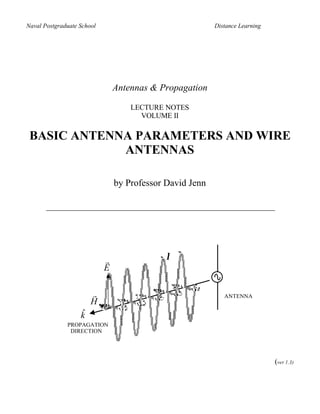
  • 1. Naval Postgraduate School Distance Learning Antennas & Propagation LECTURE NOTES VOLUME II BASIC ANTENNA PARAMETERS AND WIRE ANTENNAS by Professor David Jenn r λ E r ANTENNA H ˆ k PROPAGATION DIRECTION (ver 1.3)
  • 2. Naval Postgraduate School Antennas & Propagation Distance Learning Antennas: Introductory Comments Classification of antennas by size: Let l be the antenna dimension: 1. electrically small, l << λ : primarily used at low frequencies where the wavelength is long 2. resonant antennas, l ≈ λ / 2: most efficient; examples are slots, dipoles, patches 3. electrically large, l >> λ : can be composed of many individual resonant antennas; good for radar applications (high gain, narrow beam, low sidelobes) Classification of antennas by type: 1. reflectors 2. lenses 3. arrays Other designations: wire antennas, aperture antennas, broadband antennas 1
  • 3. Naval Postgraduate School Antennas & Propagation Distance Learning Radiation Integrals (1) Consider a perfect electric conductor (PEC) with an electric surface current flowing on S. In the case where the conductor is part of an antenna (a dipole), the current may be caused by an applied voltage, or by an incident field from another source (a reflector). The observation point is denoted by P and is given in terms of unprimed coordinate variables. Quantities associated with source points are designated by primes. We can use any coordinate system that is convenient for the particular problem at hand. OBSERVATION z POINT P ( x , y , z ) or P ( r ,θ ,φ ) r r r r r R = r − r′ r O R= R = ( x − x ′)2 + ( y − y ′)2 + ( z − z ′)2 r r′ y r x S J s ( x′, y ′, z ′) PEC WITH SURFACE CURRENT The medium is almost always free space ( µo , ε o ), but we continue to use ( µ, ε ) to cover more general problems. If the currents are known, then the field due to the currents can be determined by integration over the surface. 2
  • 4. Naval Postgraduate School Antennas & Propagation Distance Learning Radiation Integrals (2) The vector wave equation for the electric field can be obtained by taking the curl of Maxwell’s first equation: r r r ∇ × ∇ × E = k 2 E − jωµJ s r r r A solution for E in terms of the magnetic vector potential A(r ) is given by r r r r r r ∇ (∇ • A( r ) ) E ( r ) = − jωA( r ) + (1) jωµε r r r r µ J s − jkR where (r ) is a shorthand notation for (x,y,z) and A( r ) = 4π S∫∫ R e ds′ We are particularly interested in the z OBSERVATION case were the observation point is in the POINT far zone of the antenna ( P → ∞ ). As P r r r r recedes to infinity, the vectors r and R r r r r become parallel. r′ • r ˆ R ≈ r − r (r ′ • r ) ˆ ˆ r y r′ x 3
  • 5. Naval Postgraduate School Antennas & Propagation Distance Learning Radiation Integrals (3) r r In the expression for A(r ) we use the approximation 1 / R ≈ 1 / r in the denominator and r r r r • R ≈ r • [r − r(r ′ • r )] in the exponent. Equation (2) becomes ˆ ˆ ˆ ˆ r r µ r − jk r •[r − r ( r ′• r )] r r µ − jkr r jk (r ′• r ) r A( r ) ≈ ∫∫ J s e ds′ = ∫∫ J s e ds′ ˆ ˆ ˆ ˆ e 4πr S 4πr S When this is inserted into equation (1), the del operations on the second term lead to 1 / r 2 r and 1 / r 3 terms, which can be neglected in comparison to the − jωA term, which depends only on 1 / r . Therefore, in the far field, r r − jωµ − jkr r jk ( r ′• r ) E (r ) ≈ ∫∫ J s e ds′ r ˆ e (discard the E r component) (3) 4πr S Explicitly removing the r component gives, r r − jkη − jkr r r r ∫∫ [J s − r(J s • rˆ ) ]e jk ( r ′• r ) E (r ) ≈ e ˆ ˆ ds′ 4π r S The radial component of current does not contribute to the field in the far zone. 4
  • 6. Naval Postgraduate School Antennas & Propagation Distance Learning Radiation Integrals (4) r e − jkr Notice that the fields have a spherical wave behavior in the far zone: E ~ . The r r spherical components of the field can be found by the appropriate dot products with E . r More general forms of the radiation integrals that include magnetic surface currents ( J ms ) are: r − jkη − jkr  r ˆ J ms • φ  j k r ′⋅ r ˆ r Eθ ( r, θ , φ ) = ∫∫  J s •θ + ds′ ˆ 4π r e η   e S  r − jkη − jkr  r ˆ J ms • θˆ  j k r′⋅r r Eφ ( r, θ , φ ) = ∫∫  J s •φ − ds ′ ˆ 4π r e η   e S  The radiation integrals apply to an unbounded medium. For antenna problems the following process is used: 1. find the current on the antenna surface, S, 2. remove the antenna materials and assume that the currents are suspended in the unbounded medium, and 3. apply the radiation integrals. 5
  • 7. Naval Postgraduate School Antennas & Propagation Distance Learning Hertzian Dipole (1) Perhaps the simplest application of the radiation integral is the calculation of the fields of an infinitesimally short dipole (also called a Hertzian dipole). Note that the criterion for short means much less than a wavelength, which is not necessarily physically short. z • For a thin dipole (radius, a << λ ) the surface current distribution is independent of φ ′ . The current crossing a ring around 2a r the antenna is I = J s 2π a { A/m l • For a thin short dipole ( l << λ ) we assume that the current is constant and flows along z′ r the center of the wire; it is a filament of J s ( ρ ′, φ ′, z ′) = J o z ˆ zero diameter. The two-dimensional φ′ y integral over S becomes a one-dimensional ρ′ = a integral over the length, x r r ∫∫ J s ds ′ → 2πa ∫ I d l′ S L 6
  • 8. Naval Postgraduate School Antennas & Propagation Distance Learning Hertzian Dipole (2) r r Using r ′ = zz ′ and r = x sin θ cosφ + y sin θ sin φ + z cosθ gives r ′ • r = z ′ cos θ . The ˆ ˆ ˆ ˆ ˆ ˆ radiation integral for the electric field becomes r − jkη − jkr l jk (r ′• r ) − jkηI z − jkr l ˆ ′ E ( r, θ , φ ) ≈ e ∫ Ie r ˆ zdrz′ = { ˆ e ∫ e jkz cosθ dz ′ 4πr 0 dl ′ 4πr 0 However, because l is very short, kz ′ → 0 and e jkz ′ cosθ ≈ 1. Therefore, r − jkηI z − jkr l E ( r, θ , φ ) ≈ ˆ e ∫ (1) dz ′ = − jkηIl z e − jkr ˆ 4πr 0 4πr leading to the spherical field components z r ˆ • E ≈ − jkηIlθ • z e − jkr ˆ ˆ Eθ = θ 4πr l jkηIl sin θ − jkr z′ = e 4πr r x y Eφ = φˆ•E = 0 SHORT CURRENT FILAMENT 7
  • 9. Naval Postgraduate School Antennas & Propagation Distance Learning Hertzian Dipole (3) Note that the electric field has only a 1/r dependence. The absence of higher order terms is due to the fact that the dipole is infinitesimal, and therefore r ff → 0 . The field is a spherical wave and hence the TEM relationship can be used to find the magnetic field intensity r k × E r × Eθ θˆ ˆ jkIl sin θ e − jkr ˆ ˆ ˆ H= = =φ η η 4πr The time-averaged Poynting vector is r 1 ˆ r* 1 { } { Wav = ℜ E × H = ℜ Eθ Hφ r = * ˆ } ηk 2 I 2 l2 sin 2 θ r ˆ 2 2 32π r2 2 The power flow is outward from the source, as expected for a spherical wave. The average power flowing through the surface of a sphere of radius r surrounding the source is 2π π r ηk 2 I 2 l2 2π π 2 ηk 2 I 2 l2 Prad = ∫ ∫ Wav • n ds = ˆ ∫ ∫ sin θ r • rˆ r sin θ dθ dφ = 12π W ˆ 2 32π 2r 2 0 0 0 0 14444 244444 4 3 = 8π / 3 8
  • 10. Naval Postgraduate School Antennas & Propagation Distance Learning Solid Angles and Steradians Plane angles: s = Rθ , if s = R then θ = 1 radian ARC LENGTH R s θ Solid angles: Ω = A / R2 , if A = R 2 , then Ω = 1 steradian Ω = A / R2 SURFACE AREA R A 9
  • 11. Naval Postgraduate School Antennas & Propagation Distance Learning Directivity and Gain (1) The radiation intensity is defined as dPrad r 2 r U (θ , φ ) = = r r • Wav = r Wav 2 ˆ dΩ and has units of Watts/steradian (W/sr). The directivity function or directive gain is defined as r power radiated per unit solid angle dP / dΩ r 2 Wav D(θ , φ ) = = rad = 4π average power radiated per unit solid angle Prad /( 4π ) Prad For the Hertzian dipole, 2 ηk I l sin θ 2 2 2 2 r r 2 r Wav 32π 2 r 2 3 D(θ , φ ) = 4π = 4π = sin 2 θ ηk 2 I l 2 Prad 2 2 12π The directivity is the maximum value of the directive gain 3 Do = Dmax (θ ,φ ) = D (θ max ,φ max ) = 2 10
  • 12. Naval Postgraduate School Antennas & Propagation Distance Learning Dipole Polar Radiation Plots Half of the radiation pattern of the dipole is plotted below for a fixed value of φ . The half- power beamwidth (HPBW) is the angular width between the half power points (1/ 2 below the maximum on the voltage plot, or –3dB below the maximum on the decibel plot). FIELD (VOLTAGE) PLOT DECIBEL PLOT 90 1.5 90 10 120 60 120 60 0 1 150 30 150 -10 30 0.5 -20 180 θ 0 180 θ 0 210 330 210 330 240 300 240 300 270 270 The half power beamwidth of the Hertzian dipole, θ B : Enorm ~ sin θ ⇒ sin (θ HP ) = 0.707 ⇒ θ HP = 45o ⇒ θ B = 2θ HP = 90o 11
  • 13. Naval Postgraduate School Antennas & Propagation Distance Learning Dipole Radiation Pattern Radiation pattern of a Hertzian dipole aligned with the z axis. Dn is the normalized directivity. The directivity value is proportional to the distance from the center. 12
  • 14. Naval Postgraduate School Antennas & Propagation Distance Learning Directivity and Gain (2) Another formula for directive gain is 4π r 2 D(θ ,φ ) = Enorm (θ , φ ) ΩA where Ω A is the beam solid angle 2π π r 2 ΩA = ∫∫ E norm (θ , φ ) sin θ dθ dφ 0 0 r and E norm (θ ,φ ) is the normalized magnitude of the electric field pattern (i.e., the normalized radiation pattern) r r E ( r ,θ , φ ) E norm (θ , φ ) = r Emax ( r, θ , φ ) Note that both the numerator and denominator have the same 1/r dependence, and hence the ratio is independent of r. This approach is often more convenient because most of our calculations will be conducted directly with the electric field. Normalization removes all of the cumbersome constants. 13
  • 15. Naval Postgraduate School Antennas & Propagation Distance Learning Directivity and Gain (3) As an illustration, we re-compute the directivity of a Hertzian dipole. Noting that the maximum magnitude of the electric field is occurs when θ = π / 2 , the normalized electric field intensity is simply r E norm (θ ,φ ) = sin θ The beam solid angle is 2π π r 2 ΩA = ∫∫ E norm (θ , φ ) sin θ dθ dφ 0 0 π 8π = 2π ∫ sin 3 θ dθ = 3 14 4 0 2 3 =4 / 3 and from the definition of directivity, 4π r 2 4π 2 3 D(θ ,φ ) = Enorm (θ , φ ) = sin θ = sin 2 θ ΩA 8π / 3 2 which agrees with the previous result. 14
  • 16. Naval Postgraduate School Antennas & Propagation Distance Learning Example Find the directivity of an antenna whose far-electric field is given by 90 10 120 60 8 6 10e − jkr cos θ , 0o ≤ θ ≤ 90o 150 30  4  r 2 180 0 Eθ ( r, θ , φ ) =  − jkr e cos θ , 90o ≤ θ ≤ 180 o  r  210 330 240 300 r 270 The maximum electric field occurs when cosθ = 1 → Emax = 10 / r . The normalized electric field intensity is  cos θ ,  0o ≤ θ ≤ 90o Eθ norm (θ , φ ) =  0.1 cosθ , 90o ≤ θ ≤ 180o  which gives a beam solid angle of 2π π / 2 2π π 2π ΩA = ∫ ∫ cos θ sin θ dθ dφ + 0.01 ∫ ∫ cos2 θ sin θ dθ dφ = 2 (1.1) 0 0 0 π /2 3 and a directivity of Do = 5.45 = 7.37 dB. 15
  • 17. Naval Postgraduate School Antennas & Propagation Distance Learning Beam Solid Angle and Radiated Power In the far field the radiated power is 1 2π π r r  E × H *  • r ds 1 2π π r2 2 Prad = 2 ∫∫ ℜ 1 4 44 4 2 3  ˆ = 2η ∫∫ E r sin θ dθ dφ ⇒ Frad = 2ηPrad 0 0 r2 E /η 144424443 0 0 4 4 ≡ Frad From the definition of beam solid angle 2π π r 2 ΩA = ∫∫ E norm (θ , φ ) sin θ dθ dφ 0 0 1 2π π r2 2 r 2 2 2 ∫ ∫ = r E r sin θ dθ dφ = ⇒ Frad = Ω A E max r 2 E max r 1444 24444 0 0 4 3 ≡ Frad Equate the expressions for Frad r 2 Ω A E max r 2 Prad = 2η 16
  • 18. Naval Postgraduate School Antennas & Propagation Distance Learning Gain vs. Directivity (1) Directivity is defined with respect to the radiated power, Prad . This could be less than the power into the antenna if the antenna has losses. The gain is referenced to the power into the antenna, Pin . ANTENNA I Pinc Rl Pref Pin Ra Define the following: Pinc = power incident on the antenna terminals Pref = power reflected at the antenna input Pin = power into the antenna 1 2 Ploss = power loss in the antenna (dissipated in resistor Rl , Ploss = I Rl ) 2 1 2 Prad = power radiated (delivered to resistor Ra , Prad = I Ra , Ra is the radiation 2 resistance) The antenna efficiency, e, is Prad = ePin where 0 ≤ e ≤ 1 . 17
  • 19. Naval Postgraduate School Antennas & Propagation Distance Learning Gain vs. Directivity (2) Gain is defined as dPrad / dΩ dP / dΩ G (θ , φ ) = = 4π rad = eD(θ , φ ) Pin /(4π ) Prad / e Most often the use of the term gain refers to the maximum value of G(θ , φ ) . Example: The antenna input resistance is 50 ohms, of which 40 ohms is radiation resistance and 10 ohms is ohmic loss. The input current is 0.1 A and the directivity of the antenna is 2. 1 2 1 2 The input power is Pin = I Rin = 0.1 ( 50) = 0.25 W 2 2 1 2 1 2 The power dissipated in the antenna is Ploss = I Rl = 0.1 (10) = 0.05 W 2 2 1 2 1 2 The power radiated into space is Prad = I Ra = 0.1 (40 ) = 0.2 W 2 2 If the directivity is Do = 2 then the gain is G = eD =  rad  D =  P 0 .2     ( 2) = 1.6  Pin   0.25  18
  • 20. Naval Postgraduate School Antennas & Propagation Distance Learning Azimuth/Elevation Coordinate System Radars frequently use the azimuth/elevation coordinate system: (Az,El) or (α ,γ ) or (θ e , φ a ). The antenna is located at the origin of the coordinate system; the earth's surface lies in the x-y plane. Azimuth is generally measured clockwise from a reference (like a compass) but the spherical system azimuth angle φ is measured counterclockwise from the x axis. Therefore α = 360 − φ and γ = 90 − θ degrees. ZENITH z CONSTANT ELEVATION P θ r γ y φ α x HORIZON 19
  • 21. Naval Postgraduate School Antennas & Propagation Distance Learning Approximate Directivity Formula (1) Assume the antenna radiation pattern is a “pencil beam” on the horizon. The pattern is constant inside of the elevation and azimuth half power beamwidths (θ e , φa ) respectively: z θ =0 y θe x φa φ =0 θ =π /2 20
  • 22. Naval Postgraduate School Antennas & Propagation Distance Learning Approximate Directivity Formula (2) Approximate antenna pattern r  Eoe − jkr  E (θ , φ ) =  r θˆ, (π / 2 − θ e / 2 ) ≤ θ ≤ (π / 2 + θ e / 2 ) and − φa / 2 ≤ φ ≤ φa / 2 0,  else The beam solid angle is π θe φa + 2 2 2 ΩA = ∫ ∫ sin θ dθ dφ { π θe − φ − a ≈1 2 2 2 = φa [sin (θ e / 2 ) − sin (− θ e / 2 )] ≈ φa [θ e / 2 − ( −θ e / 2 )] = φaθ e 4π 4π This leads to an approximation for the directivity of Do = = . Note that the Ω A θ eφa angles are in radians. This formula is often used to estimate the directivity of an omni- directional antenna with negligible sidelobes. 21
  • 23. Naval Postgraduate School Antennas & Propagation Distance Learning Thin Wire Antennas (1) Thin wire antennas satisfy the condition a << λ . If the length of the wire (l ) is an integer multiple of a half wavelength, we can make an “educated guess” at the current based on an open circuited two-wire transmission line FEED POINTS λ /4 λ/2 z OPEN I(z) CIRCUIT For other multiples of a half wavelength the current distribution has the following features FEED POINT LOCATED AT MAXIMUM l = λ /2 l=λ CURRENT GOES TO ZERO AT END l = 3λ / 2 22
  • 24. Naval Postgraduate School Antennas & Propagation Distance Learning Thin Wire Antennas (2) On a half-wave dipole the current can be approximated by I ( z ) = I o cos( kz) for − λ / 4 < z < λ / 4 Using this current in the radiation integral r − jkη − jkr λ / 4 E ( r ,θ , φ ) = e z ∫ I o cos( kz′) e jkz ′ cosθ dz ′ ˆ 4πr −λ / 4 − jkηI o − jkr λ / 4 = e z ∫ cos( kz′) e jkz ′ cosθ dz ′ ˆ 4πr −λ / 4 From a table of integrals we find that Az ′ 6 74 4= 0 8 6= ±4 4 187 e [ A cos( Bz′) + B sin ( Bz′)] ∫ cos( Bz ′) e Az ′dz ′ = A2 + B 2 where A = jk cos θ and B = k , so that A2 + B 2 = − k 2 cos 2 θ + k 2 = k 2 sin 2 θ . The θ component requires the dot product z • θˆ = − sin θ . ˆ 23
  • 25. Naval Postgraduate School Antennas & Propagation Distance Learning Thin Wire Antennas (3) Evaluating the limits gives π 2 cos cosθ    64444 4 74444 8  4 π  2 cos cos θ  jkηI o − jkr k[e jπ cosθ / 2 − ( −1)e − jπ cosθ / 2 ] jηI o − jkr 2  Eθ = e sin θ = e 4π r k sin θ 2 2 2π r sin θ The magnetic field intensity in the far field is r π  cos cos θ  r k×E ˆ 2 φ H= ˆE jI = φ θ = o e − jkr ˆ η H φ 2πr sin θ The directivity is computed from the beam solid angle, which requires the normalized electric field intensity r 2 E norm = Eθ 2 = (π cos cos θ 2 ) 2 Eθ max 2 sin θ 24
  • 26. Naval Postgraduate School Antennas & Propagation Distance Learning Thin Wire Antennas (4) π π cos (π cos θ / 2 ) 2 cos 2 (π cos θ / 2 ) Ω A = 2π ∫ sin θ 2 sin θ dθ = 2π ∫ sin θ 2 dθ = ( 2π )(1.218) 0 1444 2444 3 0 4 4 Integrate numericall y The directive gain is D= 4π r 2 Enorm (θ , φ ) = 4π cos 2 cos θ 2 = 1.64 (π cos 2 cos θ 2 ) (π ) ΩA ( 2π )(1.218) sin 2 θ sin 2 θ The radiated power is 2 2 Ω A Eθ max r 2 2π (1.218)η 2 I o r 2 2 1 2 Prad = = = 36.57 I o ≡ I o Ra 2η 2η ( 2π r) 2 2 where Ra is the radiation resistance of the dipole. The radiated power can be viewed as the power delivered to resistor that represents “free space.” For the half-wave dipole the radiation resistance is 2P Ra = rad = ( 2 )(36.57 ) = 73.13 ohms 2 Io 25
  • 27. Naval Postgraduate School Antennas & Propagation Distance Learning Numerical Integration (1) The rectangular rule is a simple way of evaluating an integral numerically. The area under the curve of f ( x) is approximated by a sum of rectangular areas of width ∆ and height ∆ f ( xn ) , where xn = + ( n − 1) + a is the center of the interval nth interval. Therefore, if 2 all of the rectangles are of equal width b b ∫ f ( x ) dx ≈ ∆ ∑ f ( xn ) a a Clearly the approximation can be made as close to the exact value as desired by reducing the width of the triangles as necessary. However, to keep computation time to a minimum, only the smallest number of rectangles that provides a converged solution should be used. 2 3 1 4 f ( x) N ∆ L • • • x a b x1 x2 xN 26
  • 28. Naval Postgraduate School Antennas & Propagation Distance Learning Numerical Integration (2) π cos 2 (π cosθ / 2 ) Example: Matlab programs to integrate ∫ 0 sin θ dθ Sample Matlab code for the rectangular rule % integrate dipole pattern using the rectangular rule clear rad=pi/180; % avoid 0 by changing the limits slightly a=.001; b=pi-.001; N=5 delta=(b-a)/N; sum=0; for n=1:N theta=delta/2+(n-1)*delta; sum=sum+cos(pi*cos(theta)/2)^2/sin(theta); end I=sum*delta Convergence: N=5, 1.2175; N=10, 1.2187; N=50, 1.2188. Sample Matlab code using the quad8 function % integrate to find half wave dipole solid angle clear I=quad8('cint',0.0001,pi-.0001,.00001); disp(['cint integral, I: ',num2str(I)]) function P=cint(T) % function to be integrated P=(cos(pi*cos(T)/2).^2)./sin(T); 27
  • 29. Naval Postgraduate School Antennas & Propagation Distance Learning Thin Wires of Arbitrary Length For a thin-wire antenna of length l along the z axis, the electric field intensity is   kl   kl   cos cosθ  − cos   jηI − jkr   2  2 Eθ = e   2πr  sin θ      Example: l = 1.5λ (left: voltage plot; right: decibel plot) 90 2 9010 120 60 120 60 0 150 1 30 150 -10 30 -20 180 0 180 0 210 330 210 330 240 300 240 300 270 270 28
  • 30. Naval Postgraduate School Antennas & Propagation Distance Learning Feeding and Tuning Wire Antennas (1) When an antenna terminates a transmission line, as shown below, the antenna impedance ( Z a ) should be matched to the transmission line impedance ( Zo ) to maximize the power delivered to the antenna Za − Zo 1+ Γ Zo Za Γ= and VSWR = Za + Zo 1− Γ The antenna’s input impedance is generally a complex quantity, Z a = ( Ra + Rl ) + jX a . The approach for matching the antenna and increasing its efficiency is 1. minimize the ohmic loss, Rl → 0 2. “tune out” the reactance by adjusting the antenna geometry or adding lumped elements, X a → 0 (resonance occurs when Z a is real) 3. match the radiation resistance to the characteristic impedance of the line by adjusting the antenna parameters or using a transformer section, Ra → Zo 29
  • 31. Naval Postgraduate School Antennas & Propagation Distance Learning Feeding and Tuning Wire Antennas (2) Example: A half-wave dipole is fed by a 50 ohm line Z a − Z o 73 − 50 Γ= = = 0.1870 Z a + Z o 73 + 50 1+ Γ VSWR = = 1.46 1− Γ The loss due to reflection at the antenna terminals is 2 2 τ = 1 − Γ = 0.965 10 log τ ( ) = −0.155 dB 2 which is stated as “0.155 dB of reflection loss” (the negative sign is implied by using the word “loss”). 30
  • 32. Naval Postgraduate School Antennas & Propagation Distance Learning Feeding and Tuning Wire Antennas (3) The antenna impedance is affected by 1. length 2. thickness 3. shape 4. feed point (location and method of feeding) 5. end loading Although all of these parameters affect both the real and imaginary parts of Z a , they are generally used to remove the reactive part. The remaining real part can be matched using a transformer section. Another problem is encountered when matching a balanced radiating structure like a dipole to an unbalanced transmission line structure like a coax. UNBALANCED FEED BALANCED FEED COAX TWO-WIRE LINE + + λ /2 Vg λ /2 Vg − − DIPOLE DIPOLE 31
  • 33. Naval Postgraduate School Antennas & Propagation Distance Learning Feeding and Tuning Wire Antennas (4) If the two structures are not balanced, a return current can flow on the outside of the coaxial cable. These currents will radiate and modify the pattern of the antenna. The unbalanced currents can be eliminated using a balun (balanced-to-unbalanced transformer) UNBALANCED FEED BALANCED FEED I (z ) a b a b .. .. Va ≠ Vb Va = Vb Baluns frequently incorporate chokes, which are circuits designed to “choke off” current by presenting an open circuit to current waves. 32
  • 34. Naval Postgraduate School Antennas & Propagation Distance Learning Feeding and Tuning Wire Antennas (5) An example of a balun employing a choke is the sleeve or bazooka balun I2 I1 HIGH IMPEDANCE (OPEN CIRCUIT) PREVENTS CURRENT FROM FLOWING λ /4 ′ Zo ON OUTSIDE I2 I1 SHORT CIRCUIT Zo The choke prevents current from flowing on the exterior of the coax. All current is confined to the inside of surfaces of the coax, and therefore the current flow in the two directions is equal (balanced) and does not radiate. The integrity of a short circuit is easier to control than that of an open circuit, thus short circuits are used whenever possible. Originally balun referred exclusively to these types of wire feeding circuits, but the term has evolved to refer to any feed point matching circuit. 33
  • 35. Naval Postgraduate School Antennas & Propagation Distance Learning Calculation of Antenna Impedance (1) The antenna impedance must be matched to that of the feed line. The impedance of an antenna can be measured or computed. Usually measurements are more time consuming (and therefore expensive) relative to computer simulations. However, for a simulation to accurately include the effect of all of the antenna’s geometrical and electrical parameters on Z a , a fairly complicated analytical model must be used. The resulting equations must be solved numerically in most cases. One popular technique is the method of moments (MM) solution of an integral equation (IE) for the current. z 1. I (z ′) is the unknown current distribution on the l/ 2 wire 2. Find the z component of the electric field in 2a terms of I (z ′) from the radiation integral + b/ 2 3. Apply the boundary condition Vg Eg − −b / 2 0, b /2 ≤ z ≤ l / 2 Ez (ρ = a) = E , b /2 ≥ z  g −l /2 in order to obtain an integral equation for I (z ′) 34
  • 36. Naval Postgraduate School Antennas & Propagation Distance Learning Calculation of Antenna Impedance (2) One special form of the integral equation for thin wires is Pocklington’s equation  2 ∂2  l / 2 e − jkR 0, b / 2 ≤ z ≤ l / 2  k + 2  ∫ I( z ′ ) dz′ = − jωεE , b / 2 ≥ z  ∂z  −l / 2 4πR  g where R = a 2 + ( z − z ′) 2 . This is called an integral equation because the unknown quantity I (z ′) appears in the integrand. 4. Solve the integral equation using the method of moments (MM). First approximate the current by a series with unknown expansion coefficients {I n } N I( z ′ ) = ∑ InΦ n ( z ′ ) n=1 The basis functions or expansion functions {Φ n } are known and selected to suit the particular problem. We would like to use as few basis functions as possible for computational efficiency, yet enough must be used to insure convergence. 35
  • 37. Naval Postgraduate School Antennas & Propagation Distance Learning Calculation of Antenna Impedance (3) Example: a step approximation to the current using a series of pulses. Each segment is called a subdomain. Problem: there will be discontinuities between steps. I( z ′) CURRENT STEP APPROXIMATION I 2 Φ2 I1Φ1 IN Φ N ∆ L L • • • • z′ −l z1 z2 0 zN l 2 2 A better basis function is the overlapping piecewise sinusoid I( z′) CURRENT PIECEWISE SINUSOID I2 Φ2 I1Φ1 L ∆ L I NΦN • • • z′ −l z z2 0 zN l 1 2 2 36
  • 38. Naval Postgraduate School Antennas & Propagation Distance Learning Calculation of Antenna Impedance (4) A piecewise sinusoid extends over two segments (each of length ∆ ) and has a maximum at the point between the two segment  z′ − zn−1 , z ′ ≤ z ′ ≤ z ′ ′ n−1 n Φ n(z′)  z′ − zn−1 n ′   zn+1 − z ′ ′ Φ n (z ′) =  , zn ≤ z ′ ≤ zn+1 ′ ′ z′ − zn ′ z′  n+1 zn − ∆ zn z n + ∆ 0, elsewhere ( = z n −1 ) ( = zn +1 )   Φn( z′ ) Entire domain functions are also Φ1 possible. Each entire domain basis function extends over the z′ entire wire. Examples are −l Φ2 l Φ3 sinusoids. 2 2 37
  • 39. Naval Postgraduate School Antennas & Propagation Distance Learning Calculation of Antenna Impedance (5) Solving the integral equation: (1) insert the series back into the integral equation  2 ∂2  l / 2  N  e − jkR 0, b / 2 ≤ z ≤ l / 2  k + 2  ∫  ∑ InΦ n (z ′ ) dz′ = − jωεE , b / 2 ≥ z   ∂z  −l / 2  n=1  4πR  g Note that the derivative is with respect to z (not z ′ ) and therefore the differential operates only on R . For convenience we define new functions f and g: N  l / 2  2 ∂2   e − jkR ( z, z′)  0,  b/ 2 ≤ z ≤ l/ 2 ∑ I n  ∫  k + 2  Φ n ( z ′)   dz′ =  − jωεE g , b / 2 ≥ z n =1 − l / 2   4πR ( ′)   4444∂z 4 24444z, z44  4444 244444 1 4 4 4 3 1 4 3 ≡ f ( Φ n )→ f n ( z ) ≡g Once Φ n is defined, the integral can be evaluated numerically. The result will still be a function of z, hence the notation f n (z ) . (2) Choose a set of N testing (or weighting) functions {Χ m }. Multiply both sides of the equation by each testing function and integrate over the domain of each function ∆ m to obtain N equations of the form ∫ Χ m ( z )n∑1I n f n (z ) dz = ∫ Χ m (z ) g (z )dz , N m = 1,2,..., N = ∆m ∆m 38
  • 40. Naval Postgraduate School Antennas & Propagation Distance Learning Calculation of Antenna Impedance (6) Interchange the summation and integration operations and define new impedance and voltage quantities N     ∑ ∫ ∫ I n  Χ m ( z) f mn ( z) dz  = Χ m ( z) g ( z)dz n =1 ∆ m  444 444  ∆ m44 44  1 2 3 1 2 3 Z mn Vm This can be cast into the form of a matrix equation and solved using standard matrix methods N ∑ In Zmn = Vm → [ Z][I ] = [V ] → [ I ] = [Z ]−1[V ] n=1 [Z ] is a square impedance matrix that depends only on the geometry and material characteristics of the dipole. Physically, it is a measure of the interaction between the currents on segments m and n. [V ] is the excitation vector. It depends on the field in the gap and the chosen basis functions. [I ] is the unknown current coefficient vector. After [I ] has been determined, the resulting current series can be inserted in the radiation integral, and the far fields computed by integration of the current. 39
  • 41. Naval Postgraduate School Antennas & Propagation Distance Learning Self-Impedance of a Wire Antenna The method of moments current allows calculation of the self impedance of the antenna by taking the ratio Zself = Vg / Io RESISTANCE REACTANCE 40
  • 42. Naval Postgraduate School Antennas & Propagation Distance Learning The Fourier Series Analog to MM The method of moments is a general solution method that is widely used in all of engineering. A Fourier series approximation to a periodic time function has the same solution process as the MM solution for current. Let f (t ) be the time waveform ao 2 ∞ f (t) = + ∑ [an cos(ω nt ) + bn sin (ω nt )] T T n =1 For simplicity, assume that there is no DC component and that only cosines are necessary to represent f (t ) (true if the waveform has the right symmetry characteristics) 2 ∞ f ( t ) = ∑ an cos(ωn t ) T n =1 The constants are obtained by multiplying each side by the testing function cos(ω m t) and integrating over a period 0, m ≠ n 2 T /2  ∞ (ω nt ) cos(ω mt ) dt =  T /2 ∫ f ( t ) cos(ω mt )dt = ∫  ∑ a cos   −T / 2 T −T / 2  n =1 n  an , m = n This is analogous to MM when f ( t ) → I ( z ′) , a n → I n , Φ n → cos(ωn t ) , and Χ m → cos(ωm t ) . (Since f (t ) is not in an integral equation, a second variable t ′ is not required.) The selection of the testing functions to be the complex conjugates of the expansion functions is referred to as Galerkin’s method. 41
  • 43. Naval Postgraduate School Antennas & Propagation Distance Learning Reciprocity (1) When two antennas are in close proximity to each other, there is a strong interaction between them. The radiation from one affects the current distribution of the other, which in turn modifies the current distribution of the first one. ANTENNA 1 ANTENNA 2 (SOURCE) (RECEIVER) I1 I2 + V1 Eg V21 − Z1 Z2 Consider two situations (depicted on the following page) where the geometrical relationship between two antennas does not change. 1. A voltage is applied to antenna 1 and the current induced at the terminals of antenna 2 is measured. 2. The situation is reversed: a voltage is applied to antenna 2 and the current induced at the terminals of antenna 1 is measured. 42
  • 44. Naval Postgraduate School Antennas & Propagation Distance Learning Reciprocity (2) Case 1: ANTENNA 1 I2 CURRENT METER + V1 ENERGY FLOW − ANTENNA 2 Case 2: ANTENNA 1 + V2 − I1 ENERGY FLOW ANTENNA 2 CURRENT METER 43
  • 45. Naval Postgraduate School Antennas & Propagation Distance Learning Mutual Impedance (1) Define the mutual impedance or transfer impedance as V2 V Z12 = and Z21 = 1 I1 I2 The first index on Z refers to the receiving antenna (observer) and the second index to the source antenna. Reciprocity Theorem: If the antennas and medium are linear, passive and isotropic, then the response of a system to a source is unchanged if the source and observer (measurer) are interchanged. With regard to mutual impedance: • This implies that Z21 = Z12 • The receiving and transmitting patterns of an antenna are the same if it is constructed of linear, passive, and isotropic materials and devices. In general, the input impedance of antenna number n in the presence of other antennas is obtained by integrating the total field in the gap (gap width bn ) Vn 1 r r Zn = = ∫ En • dl In In bn 44
  • 46. Naval Postgraduate School Antennas & Propagation Distance Learning Mutual Impedance (2) r En is the total field in the gap of antenna n (due to its own voltage plus the incident fields from all other antennas). Vn En In 45
  • 47. Naval Postgraduate School Antennas & Propagation Distance Learning Mutual Impedance (3) If there are a total of N antennas r r r r En = En1 + En2 + L + EnN Therefore, 1 N r r In ∫ m=1 nm Zn = ∑ E • dln bn Define r r Vnm = ∫ E nm• d ln bn The impedance becomes 1 N N V N Zn = ∑ Vnm = ∑ nm = ∑ Z nm I n m =23 m =1 I n m =1 11 { ≡Vn ≡ Z nm For example, the impedance of dipole n=1 is written explicitly as Z1 = Z11 + Z12 + L+ Z1N When m = n the impedance is the self impedance. This is approximately the impedance that we have already computed for an isolated dipole using the method of moments. 46
  • 48. Naval Postgraduate School Antennas & Propagation Distance Learning Mutual Impedance (4) The method of moments can also be used to compute the mutual coupling between antennas. The mutual impedance is obtained from the definition Vm mutual impedance at port m due to a Zmn = = In current in port n, with port m open ciruited I m =0 Vn By reciprocity this is the same as Zmn = Znm = . Say that we have two dipoles, one Im In =0 distant (n) and one near (m). To determine Zmn a voltage can be applied to the distant dipole and the open-circuited current computed on the near dipole using the method of moments. The ratio of the distant dipole’s voltage to the current induced on the near one gives the mutual impedance between the two dipoles. Plots of mutual impedance are shown on the following pages: 1. high mutual impedance implies strong coupling between the antennas 2. mutual impedance decreases with increasing separation between antennas 3. mutual impedance for wire antennas placed end to end is not as strong as when they are placed parallel 47
  • 49. Naval Postgraduate School Antennas & Propagation Distance Learning Mutual Impedance of Parallel Dipoles 80 60 λ /2 d 40 R12 R or X (ohms) 20 0 X 12 -20 -40 0 0.5 1 1.5 2 Separation, d (wavelengths) 48
  • 50. Naval Postgraduate School Antennas & Propagation Distance Learning Mutual Impedance of Colinear Dipoles 25 λ /2 20 s 15 R or X (ohms) 10 R21 5 0 X 21 -5 -10 0 0.5 1 1.5 2 Separation, s (wavelengths) 49
  • 51. Naval Postgraduate School Antennas & Propagation Distance Learning Mutual-Impedance Example Example: Assume that a half wave dipole has been tuned so that it is resonant ( Xa = 0). We found that a resonant half wave dipole fed by a 50 ohm transmission line has a VSWR of 1.46 (a reflection coefficient of 0.1870). If a second half wave dipole is placed parallel to the first one and 0.65 wavelength away, what is the input impedance of the first dipole? From the plots, the mutual impedance between two dipoles spaced 0.65 wavelength is Z21 = R21 + jX21 = −24.98 − j7.7Ω Noting that Z 21 = Z12 the total input impedance is Zin = Z11 + Z21 = 73 + (−24.98 − j7.7) = 48.02 − j7.7 Ω The reflection coefficient is Zin − Zo (48.02 − j7.7) − 50 − j99.93 o Γ= = = −0.0139 − j0.0797 = 0.081e Zin + Zo (48.02 − j7.7) + 50 which corresponds to a VSWR of 1.176. In this case the presence of the second dipole has improved the match at the input terminals of the first antenna. 50
  • 52. Naval Postgraduate School Antennas & Propagation Distance Learning Broadband Antennas (1) The required frequency bandwidth increases with the rate of information transfer (i.e., high data rates require wide frequency bandwidths). Designing an efficient wideband antenna is difficult. The most efficient antennas are designed to operate at a resonant frequency, which is inherently narrow band. Two approaches to operating over wide frequency bands: 1. Split the entire band into sub-bands and use a separate resonant antenna in each band Advantage: The individual antennas are easy to design (potentially inexpensive) Disadvantage: Many antennas are required (may take a lot of space, weight, etc.) TOTAL SYSTEM BANDWIDTH OF AN BANDWIDTH 1 ∆f1 INDIVIDUAL ANTENNA MULTIPLEXER FREQUENCY BROADBAND INPUT SIGNAL 2 ∆f2 τ L M f N ∆f N ∆f1 ∆f2 ∆f N 51
  • 53. Naval Postgraduate School Antennas & Propagation Distance Learning Broadband Antennas (2) 2. Use a single antenna that operates over the entire frequency band Advantage: Less aperture area required by a single antenna Disadvantage: A wideband antenna is more difficult to design than a narrowband antenna Broadbanding of antennas can be accomplished by: 1. interlacing narrowband elements having non-overlapping sub-bands (stepped band approach) Example: multi-feed point dipole TANK CIRCUIT USING LUMPED ELEMENTS d min OPEN CIRCUIT AT HIGH FREQUENCIES d max SHORT CIRCUIT AT LOW FREQUENCIES 52
  • 54. Naval Postgraduate School Antennas & Propagation Distance Learning Broadband Antennas (3) 2. design elements that have smooth geometrical transitions and avoid abrupt discontinuities Example: biconical antenna d min d max spiral antenna dmax FEED POINT d min WIRES 53
  • 55. Naval Postgraduate School Antennas & Propagation Distance Learning Circular Spiral in Low Observable Fixture 54
  • 56. Naval Postgraduate School Antennas & Propagation Distance Learning Broadband Antennas (4) Another example of a broadband antenna is the log-periodic array. It can be classified as a single element with a gradual geometric transitions or as discrete elements that are resonant in sub-bands. All of the elements of the log periodic antenna are fed. DIRECTION d min d max OF MAXIMUM RADIATION The range of frequencies over which ana antenna operates is determined approximately by the maximum and minimum antenna dimensions λH λ dmin ≈ and dmax ≈ L 2 2 55
  • 57. Naval Postgraduate School Antennas & Propagation Distance Learning Yagi-Uda Antenna A Yagi-Uda (or simply Yagi) is used at high frequencies (HF) to obtain a directional azimuth pattern. They are frequently employed as TV/FM antennas. A Yagi consists of a fed element and at least two parasitic (non-excited) elements. The shorter elements in the front are directors. The longer element in the back is a reflector. The conventional design has only one reflector, but may have up to 10 directors. POLAR PLOT OF RADIATION PATTERN REFLECTOR DIRECTORS BACK LOBE MAIN LOBE FED MAXIMUM MAXIMUM ELEMENT DIRECTIVITY DIRECTIVITY The front-to-back ratio is the ratio of the maximum directivity in the forward direction to that in the back direction: Dmax / Dback 56
  • 58. Naval Postgraduate School Antennas & Propagation Distance Learning Ground Planes and Images (1) In some cases the method of images allows construction of an equivalent problem that is easier to solve than the original problem. When a source is located over a PEC ground plane, the ground plane can be removed and the effects of the ground plane on the fields outside of the medium accounted for by an image located below the surface. ORIGINAL PROBLEM EQUIVALENT PROBLEM ORIGINAL → → SOURCES → → h I dl I dl I dl h I dl REGION 1 GROUND PLANE PEC REMOVED REGION 2 h IMAGE SOURCES → → I dl I dl The equivalent problem holds only for computing the fields in region 1. It is exact for an infinite PEC ground plane, but is often used for finite, imperfectly conducting ground planes (such as the Earth’s surface). 57
  • 59. Naval Postgraduate School Antennas & Propagation Distance Learning Ground Planes and Images (2) The equivalent problem satisfies Maxwell’s equations and the same boundary conditions as the original problem. The uniqueness theorem of electromagnetics assures us that the solution to the equivalent problem is the same as that for the original problem. Boundary conditions at the surface of a PEC: the tangential component of the electric field is zero. ORIGINAL PROBLEM EQUIVALENT PROBLEM → → Idz TANGENTIAL Idz θ1 COMPONENTS CANCEL h h E|| =0 PEC Eθ E⊥ h θ2 Eθ1 Eθ 2 → Idz A similar result can be shown if the current element is oriented horizontal to the ground plane and the image is reversed from the source. (A reversal of the image current direction implies a negative sign in the image’s field relative to the source field.) 58
  • 60. Naval Postgraduate School Antennas & Propagation Distance Learning Ground Planes and Images (3) Half of a symmetric conducting structure can be removed if an infinite PEC is placed on the symmetry plane. This is the basis of a quarter-wave monopole antenna. I λ /4 I λ/4 + + Vg b Vg 2b z=0 − PEC − ORIGINAL MONOPOLE DIPOLE • The radiation pattern is the same for the monopole as it is for the half wave dipole above the plane z = 0 • The field in the monopole gap is twice the field in the gap of the dipole • Since the voltage is the same but the gap is half of the dipole’s gap 1 73.12 Ra monopole = Ra dipole = = 36.56 ohms 2 2 59