Error detection and correction

1. Error Detection and Correction
Environmental interference and physical defects in the communication medium can cause
random bit errors during data transmission. Error coding is a method of detecting and correcting
these errors to ensure information is transferred intact from its source to its destination.
Error coding is used for fault tolerant computing in computer memory, magnetic and optical data
storage media, satellite and deep space communications, network communications, cellular
telephone networks, and almost any other form of digital data communication. Error coding uses
mathematical formulas to encode data bits at the source into longer bit words for transmission.
The "code word" can then be decoded at the destination to retrieve the information. The extra
bits in the code word provide redundancy that, according to the coding scheme used, will allow
the destination to use the decoding process to determine if the communication medium
introduced errors and in some cases correct them so that the data need not be retransmitted.
1.1 Types of errors
These interferences can change the timing and shape of the signal. If the signal is carrying binary
encoded data, such changes can alter the meaning of the data. These errors can be divided into
two types: Single-bit error and Burst error.
Single-bit Error
The term single-bit error means that only one bit of given data unit (such as a byte, character, or
data unit) is changed from 1 to 0 or from 0 to 1 as shown in Fig. 1.1.1
Fig.1.1.1 Single bit error
Example:
Single bit errors are least likely type of errors in serial data transmission. To see why, imagine a
sender sends data at 10 Mbps. This means that each bit lasts only for 0.1 μs (micro-second). For
a single bit error to occur noise must have duration of only 0.1 μs (micro-second), which is very
rare. However, a single-bit error can happen if we are having a parallel data transmission. For
example, if 16 wires are used to send all 16 bits of a word at the same time and one of the wires
is noisy, one bit is corrupted in each word.
Burst Error
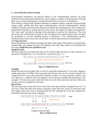
The term burst error means that two or more bits in the data unit have changed from 0 to 1 or
vice-versa. Note that burst error doesn’t necessary means that error occurs in consecutive bits.
The length of the burst error is measured from the first corrupted bit to the last corrupted bit.
Some bits in between may not be corrupted.
Fig.1.1.2 Burst Error

Example:
Burst errors are mostly likely to happen in serial transmission. The duration of the noise is
normally longer than the duration of a single bit, which means that the noise affects data; it
affects a set of bits as shown in Fig. 1.1.2. The number of bits affected depends on the data rate
and duration of noise.
Error-Correcting Codes
One way is to include enough redundant information (extra bits are introduced into the data
stream at the transmitter on a regular and logical basis) along with each block of data sent to
enable the receiver to deduce what the transmitted character must have been. This method
sometimes called forward error correction.
Error-detecting Codes.
The other way is to include only enough redundancy to allow the receiver to deduce that error
has occurred, but not which error has occurred and the receiver asks for a retransmission.
1.2 Error Detecting Codes
Basic approach used for error detection is the use of redundancy, where additional bits are added
to facilitate detection and correction of errors. Popular techniques are:
Simple Parity check
Two-dimensional Parity check
Checksum
Cyclic redundancy check
1.2.1 Simple Parity Checking or One-dimension Parity Check
The most common and least expensive mechanism for error- detection is the simple parity check.
In this technique, a redundant bit called parity bit, is appended to every data unit so that the
number of 1s in the unit (including the parity bit) becomes even.
Blocks of data from the source are subjected to a check bit or Parity bit generator form, where a
parity of 1 is added to the block if it contains an odd number of 1’s (ON bits) and 0 is added if it
contains an even number of 1’s. At the receiving end the parity bit is computed from the received
data bits and compared with the received parity bit, as shown in Fig. 1.2.1. This scheme makes
the total number of 1’s even, that is why it is called even parity checking.
Fig. 1.2.1 Even-parity checking scheme

Note that for the sake of simplicity, we are discussing here the even-parity checking, where the
number of 1’s should be an even number. It is also possible to use odd-parity checking, where the
number of 1’s should be odd.
Performance
Simple parity check scheme can detect single bit error. However, if two errors occur in the code
word, it becomes another valid member of the set and the decoder will see only another valid
code word and know nothing of the error. Thus errors in more than one bit cannot be detected. In
fact it can be shown that a single parity check code can detect only odd number of errors in a
code word.
1.2.2 Two-dimension Parity Check
Performance can be improved by using two-dimensional parity check, which organizes the block of
bits in the form of a table. Parity check bits are calculated for each row, which is equivalent to a
simple parity check bit. Parity check bits are also calculated for all columns then both are sent along
with the data. At the receiving end these are compared with the parity bits calculated on the received
data.
Fig. 1.2.2 Two-dimension Parity Checking
Performance
Two- Dimension Parity Checking increases the likelihood of detecting burst errors. A burst error of
more than n bits is also detected by 2-D Parity check with a high-probability. There is, however, one
pattern of error that remains elusive.
1.2.3 Checksum
In checksum error detection scheme, the data is divided into k segments each of m bits. In the
sender’s end the segments are added using 1’s complement arithmetic to get the sum. The sum is
complemented to get the checksum. The checksum segment is sent along with the data segments
as shown in Fig. 1.2.3 (a). At the receiver’s end, all received segments are added using 1’s
complement arithmetic to get the sum. The sum is complemented. If the result is zero, the
received data is accepted; otherwise discarded, as shown in Fig. 1.2.3 (b).
Performance
The checksum detects all errors involving an odd number of bits. It also detects most errors involving
even number of bits.

(a) (b)
Figure 1.2.3 (a) Sender’s end for the calculation of the checksum, (b) Receiving end for
checking the checksum
1.2.4 Cyclic Redundancy Checks (CRC)
This Cyclic Redundancy Check is the most powerful and easy to implement technique. Unlike
checksum scheme, which is based on addition, CRC is based on binary division. In CRC, a
sequence of redundant bits, called cyclic redundancy check bits, are appended to the end of
data unit so that the resulting data unit becomes exactly divisible by a second, predetermined
binary number. At the destination, the incoming data unit is divided by the same number. If at
this step there is no remainder, the data unit is assumed to be correct and is therefore accepted. A
remainder indicates that the data unit has been damaged in transit and therefore must be rejected.
The generalized technique can be explained as follows.
If a k bit message is to be transmitted, the transmitter generates an r-bit sequence, known as
Frame Check Sequence (FCS) so that the (k+r) bits are actually being transmitted. Now this r-bit
FCS is generated by dividing the original number, appended by r zeros, by a predetermined
number. This number, which is (r+1) bit in length, can also be considered as the coefficients of a
polynomial, called Generator Polynomial. The remainder of this division process generates the
r-bit FCS. On receiving the packet, the receiver divides the (k+r) bit frame by the same
predetermined number and if it produces no remainder, it can be assumed that no error has
occurred during the transmission. Operations at both the sender and receiver end are shown in
Fig. 1.2.4

.
Fig. 1.2.4 Basic scheme for Cyclic Redundancy Checking
This mathematical operation performed is illustrated in Fig. 1.2.4 by dividing a sample 4-bit number
by the coefficient of the generator polynomial x3+x+1, which is 1011, using the modulo-2 arithmetic.
Modulo-2 arithmetic is a binary addition process without any carry over, which is just the Exclusive-
OR operation. Consider the case where k=1101. Hence we have to divide 1101000 (i.e. k appended
by 3 zeros) by 1011, which produces the remainder r=001, so that the bit frame (k+r) =1101001 is
actually being transmitted through the communication channel. At the receiving end, if the received
number, i.e., 1101001 is divided by the same generator polynomial 1011 to get the remainder as 000,
it can be assumed that the data is free of errors.
Fig. 1.2.4 Cyclic Redundancy Checks
All the values can be expressed as polynomials of a dummy variable X. For example, for P = 11001
the corresponding polynomial is X4+X3+1. A polynomial is selected to have at least the following
properties:
It should not be divisible by X.
It should not be divisible by (X+1).
The first condition guarantees that all burst errors of a length equal to the degree of polynomial are
detected. The second condition guarantees that all burst errors affecting an odd number of bits are
detected.

In a cyclic code, where s(x) is the syndrome
If s(x) ≠ 0, one or more bits is corrupted.
If s(x) = 0, either
a. No bit is corrupted. or
b. Some bits are corrupted, but the decoder failed to detect them.
Performance
CRC is a very effective error detection technique. If the divisor is chosen according to the
previously mentioned rules, its performance can be summarized as follows:
CRC can detect all single-bit errors
CRC can detect all double-bit errors (three 1’s)
CRC can detect any odd number of errors (X+1)
CRC can detect all burst errors of less than the degree of the polynomial.
CRC detects most of the larger burst errors with a high probability.
2. Framing and synchronization
Normally, units of data transfer are larger than a single analog or digital encoding symbol. It is
necessary to recover clock information for both the signal and obtain synchronization for larger
units of data (such as data words and frames). It is necessary to recover the data in words or
blocks because this is the only way the receiver process will be able to interpret the data
received; for a given bit stream. So, it is necessary to add other bits to the block that convey
control information used in the data link control procedures. The data along with preamble,
postamble, and control information forms a frame. Frame synchronization or delineation (or
simply framing) is theprocess of defining and locating frame boundaries (start and end ofthe
frame) on a bit sequence. This framing is necessary for the purpose of synchronization and other
data control functions.
Framing Method
The problem of framing is solved in different ways depending on theframes having a fixed
(known) length or a variable length
For frames of fixed length (e.g., a physical layer SONET/SDH frame or an ATM cell), it is
only necessary to identify the start of the frame and add the frame size to locate the end of
the frame – framing methods can thus exploit the occurrence of either periodic patterns or
known correlations that occur periodically in bit sequences (the latter is exploited in ATM)
For frames of variable size, special synchronization characters or bit patterns are used to
identify the start of a frame, while different explicit or implicit methods can be used for
identifying the end of a frame (e.g., special characters or bit patterns, a length field or some
event that may be associated with the end of the frame)
2.1 Character oriented framing
Character-oriented protocols are also known as byte oriented protocols. They are used in variable
size framing by the Data link layer for data link control. Data are 8-bit characters encoded in
ASCII. Along with the header and the trailer, 2 flags are included in each frame (beginning and
end of frame) to separate it from other frames.
To separate one frame from the next an 8bit(1-byte) flag is added at the beginning and the end
of a frame. The flag is protocol dependent special characters, signals the start or end of a frame.

But same type of special character pattern may appear at the middle of the data and receiver thins
that it reached the end of the frame. To resolve this problem, a byte stuffing strategy was added
to character oriented framing. In byte stuffing (or character stuffing), a special byte is added to
the data section of the frame when there is a character with the same patter as the flag. The data
section is stuffed by an extra byte. This byte is usually called escape character (ESC) which has a
predefined bit pattern. Whenever the receiver encounters the ESC character, it removes it from
the data section and treats the next character as data, not a delaminating flag.
If there is also one or more ESC in the frame followed by flag. The receiver removes the ESC
and keeps the flag which is incorrectly interpreted as the end of the frame. To solve this problem
The ESC character which is part of the text must also be marked by another ESC as shown in fig.
2.1.1
Fig.2.1.1 Byte stuffing and unstuffing
Disadvantage:
Clearly, this procedure does not account for universal coding system, such as Unicode, have
16-bit or 32-bit characters that conflict with 8-bit character, so we rely on bit-stuffing
protocols (mostly).
More you do byte stuffing more bandwidth is required to represent the data.
2.2 Bit Oriented framing
If the flag pattern appears anywhere in the header or data of a frame, then the receiver may
prematurely detect the start or end of the received frame. To overcome this problem, the sender
makes sure that the frame body it sends has no flags in it at any position (note that since there is
no character synchronization, the flag pattern can start at any bit location within the stream). It
does this by bit stuffing, inserting an extra bit in any pattern that is beginning to look like a flag.
In HDLC, whenever 5 consecutive 1's are encountered in the data, a 0 is inserted after the 5th 1,
regardless of the next bit in the data as shown in Fig. 2.2.1. On the receiving end, the bit stream
is piped through a shift register as the receiver looks for the flag pattern. If 5 consecutive 1's
followed by a 0 is seen, then the 0 is dropped before sending the data on (the receiver destuffs
the stream). If 6 1's and a 0 are seen, it is a flag and either the current frame are ended or a new
frame is started, depending on the current state of the receiver. If more than 6 consecutive 1's are
seen, then the receiver has detected an invalid pattern, and usually the current frame, if any, is
discarded.
Bit stuffing is the process of adding one extra 0 whenever five consecutive 1s follow a 0 in the
data, so that the receiver does not mistakethe pattern 0111110 for a flag.

Fig.2.2.1 Bit stuffing and unstuffing
3. Flow Control and Error Control
The most important functions of Data Link layer to satisfy the above requirements are error
control and flow control. Collectively, these functions are known as data link control.
Flow Control is a technique so that transmitter and receiver with different speed characteristics can
communicate with each other. Flow control ensures that a transmitting station, such as a server with
higher processing capability, does not overwhelm a receiving station, such as a desktop system, with
lesser processing capability. This is where there is an orderly flow of transmitted data between the
source and the destination.
Error Control involves both error detection and error correction. It is necessary because errors
are inevitable in data communication, in spite of the use of better equipment and reliable
transmission media based on the current technology. When an error is detected, the receiver can
have the specified frame retransmitted by the sender. This process is commonly known as
Automatic Repeat Request (ARQ). For example, Internet's Unreliable Delivery Model allows
packets to be discarded if network resources are not available, and demands that ARQ protocols
make provisions for retransmission.
Modern data networks are designed to support a diverse range of hosts and communication
mediums. Consider a 933 MHz Pentium-based host transmitting data to a 90 MHz 80486/SX.
Obviously, the Pentium will be able to drown the slower processor with data. Likewise, consider
two hosts, each using an Ethernet LAN, but with the two Ethernets connected by a 56 Kbps
modem link. If one host begins transmitting to the other at Ethernet speeds, the modem link will
quickly become overwhelmed. In both cases, flow control is needed to pace the data transfer at
an acceptable speed.
3.1 Protocols for Flow Control
Flow control refers to the set of procedures used to restrict the amount of data the transmitter
can send before waiting for acknowledgment. The flow of data should not be allowed to
overwhelm the receiver. Receiver should also be able to inform the transmitter before its limits
are reached and the sender must send fewer frames.
There are two methods developed for flow control namely Stop-and-wait and Sliding-window.
Stop-and-wait is also known as Request/reply sometimes. Request/reply (Stop-and-wait) flow
control requires each data packet to be acknowledged by the remote host before the next packet
is sent.

Sliding window algorithms, used by TCP, permit multiple data packets to be in simultaneous
transmit, making more efficient use of network bandwidth.
3.1.1 Stop-and-Wait
This is the simplest form of flow control where a sender transmits a data frame. After receiving
the frame, the receiver indicates its willingness to accept another frame by sending back an ACK
frame acknowledging the frame just received. The sender must wait until it receives the ACK
frame before sending the next data frame. This is sometimes referred as request/reply, is simple
to understand and easy to implement, but not very efficient. In LAN environment with fast links,
this isn't much of a concern, but WAN links will spend most of their time idle, especially if
several hops are required.
Figure 3.1.1 illustrates the operation of the stop-and-wait protocol. The blue arrows show the
sequence of data frames being sent across the link from the sender (top to the receiver (bottom).
The protocol relies on two-way transmission (full duplex or half duplex) to allow the receiver at
the remote node to return frames acknowledging the successful transmission. The
acknowledgements are shown in green in the diagram, and flow back to the original sender. A
small processing delay may be introduced between reception of the last byte of a Data PDU and
generation of the corresponding ACK.
Fig. 3.1.1 Stop-and Wait protocol
Example:Internet's Remote Procedure Call (RPC) Protocol is used to implement subroutine calls
from a program on one machine to library routines on another machine.
Drawback
Major drawback of Stop-and-Wait Flow Control is that only one frame can be in transmission at a
time, this leads to inefficiency if propagation delay is much longer than the transmission delay.
Link Utilization in Stop-and-Wait
Let us assume the following:
Transmission time: The time it takes for a station to transmit a frame (normalized to a value of 1).
Propagation delay: The time it takes for a bit to travel from sender to receiver (expressed as a).
a< 1 :The frame is sufficiently long such that the first bits of the frame arrive at the
destination before the source has completed transmission of the frame.
a> 1: Sender completes transmission of the entire frame before the leading bits of the frame
arrive at the receiver.
The link utilization U = 1/(1+2a),
a = Propagation time / transmission time

It is evident from the above equation that the link utilization is strongly dependent on the ratio of the
propagation time to the transmission time. When the propagation time is small, as in case of LAN
environment, the link utilization is good. But, in case of long propagation delays, as in case of
satellite communication, the utilization can be very poor. To improve the link utilization, we can use
the following (sliding-window) protocol instead of using stop-and-wait protocol.
3.1.2 Sliding Window
With the use of multiple frames for a single message, the stop-and-wait protocol does not
perform well. Only one frame at a time can be in transit. In stop-and-wait flow control, if a > 1,
serious inefficiencies result. Efficiency can be greatly improved by allowing multiple frames to
be in transit at the same time. Efficiency can also be improved by making use of the full-duplex
line. To keep track of the frames, sender station sends sequentially numbered frames. Since the
sequence number to be used occupies a field in the frame, it should be of limited size. If the
header of the frame allows k bits, the sequence numbers range from 0 to 2k
– 1. Sender maintains
a list of sequence numbers that it is allowed to send (sender window). The size of the sender’s
window is at most 2k
– 1. The sender is provided with a buffer equal to the window size.
Receiver may also maintain a window of size at most 2k
– 1. The receiver acknowledges a frame
by sending an ACK frame that includes the sequence number of the next frame expected. This
also explicitly announces that it is prepared to receive the next N frames, beginning with the
number specified. This scheme can be used to acknowledge multiple frames. It could receive
frames 2, 3, 4 but withhold ACK until frame 4 has arrived. By returning an ACK with sequence
number 5, it acknowledges frames 2, 3, 4 in one go. The receiver needs a buffer of size 1.
Sliding window algorithm is a method of flow control for network data transfers. TCP, the Internet's
stream transfer protocol, uses a sliding window algorithm.
Sender sliding Window: with sequence
numbers in a certain range (the sending window) as shown in Fig. 3.1.2.
Fig. 3.1.2 Sender’s window
Receiver sliding Window: The receiver always maintains a window of size 1 as shown in Fig.
3.1.3. It looks for a specific frame (frame 4 as shown in the figure) to arrive in a specific order. If
it receives any other frame (out of order), it is discarded and it needs to be resent. However, the
receiver window also slides by one as the specific frame is received and accepted as shown in the
figure. The receiver acknowledges a frame by sending an ACK frame that includes the sequence

number of the next frame expected. This also explicitly announces that it is prepared to receive
the next N frames, beginning with the number specified. This scheme can be used to
acknowledge multiple frames. It could receive frames 2, 3, 4 but withhold ACK until frame 4 has
arrived. By returning an ACK with sequence number 5, it acknowledges frames 2, 3, 4 at one
time. The receiver needs a buffer of size 1.
Fig. 3.1.3 Receiver sliding window
Hence, Sliding Window Flow Control
Allows transmission of multiple frames
Assigns each frame a k-bit sequence number
Range of sequence number is [0…2k
-1], i.e., frames are counted modulo 2k
.
The link utilization in case of Sliding Window Protocol
U = 1, for N > 2a + 1
N/(1+2a), for N < 2a + 1
Where N = the window size, and a = Propagation time / transmission time
Data Link layer can combine framing, flow control and error control to achieve the delivery of
data from one node to another node. The most popular retransmission scheme is known as
Automatic-Repeat-Request (ARQ). Such schemes, where receiver asks transmitter to re-transmit
if it detects an error, are known as reverse error correction techniques.
4. Error Control Techniques
When an error is detected in a message, the receiver sends a request to the transmitter to retransmit
the ill-fated message or packet. The most popular retransmission scheme is known as Automatic-
Repeat-Request (ARQ). Such schemes, where receiver asks transmitter to re-transmit if it detects an
error, are known as reverse error correction techniques. There exist three popular ARQ techniques, as
shown in Fig. 4.1.1.
Fig. 4.1.1 Error control techniques
4.1.1 Stop-and-Wait ARQ
In Stop-and-Wait ARQ, which is simplest among all protocols, the sender (say station A) transmits a
frame and then waits till it receives positive acknowledgement (ACK) or negative acknowledgement
(NACK) from the receiver (say station B). Station B sends an ACK if the frame is received correctly,

otherwise it sends NACK. Station A sends a new frame after receiving ACK; otherwise it retransmits
the old frame, if it receives a NACK. This is illustrated in Fig 4.1.2.
Fig. 4.1.2Stop-And-Wait ARQ technique
To tackle the problem of a lost or damaged frame, the sender is equipped with a timer. In case of
a lost ACK, the sender transmits the old frame. In the Fig. 4.1.3, the second PDU of Data is lost
during transmission. The sender is unaware of this loss, but starts a timer after sending each
PDU. Normally an ACK PDU is received before the timer expires. In this case no ACK is
received, and the timer counts down to zero and triggers retransmission of the same PDU by the
sender. The sender always starts a timer following transmission, but in the second transmission
receives an ACK PDU before the timer expires, finally indicating that the data has now been
received by the remote node.The receiver now can identify that it has received a duplicate frame
from the label of the frame and it is discarded.
Figure 4.1.3 shows an example of Stop-and-Wait ARQ. Frame 0 is sent and acknowledged.
Frame 1 is lost and resent after the time-out. The resent frame 1 is acknowledged and the timer
stops. Frame 0 is sent and acknowledged, but the acknowledgment is lost. The sender has no idea
if the frame or the acknowledgment is lost, so after the time-out, it resends frame 0, which is
acknowledged.
Fig. 4.1.3 Flow diagram for an example of Stop-and-Wait ARQ

The main advantage of stop-and-wait ARQ is its simplicity. It also requires minimum buffer size.
However, it makes highly inefficient use of communication links, particularly when ‘a’ is large.
The stop-and wait ARQ is inefficient if the channel is thick and long, that means the channel has
large bandwidth and the round trip delay is long. The product of the two is called the bandwidth
product delay.
Example: Assume that, in a Stop-and-Wait ARQ system, the bandwidth of the line is 1 Mbps,
and 1 bit takes 20 ms to make a round trip. What is the bandwidth-delay product? If the system
data frames are 1000 bits in length, what is the utilization percentage of the link?
Solution
The bandwidth-delay product is
The system can send 20,000 bits during the time it takes for the data to go from the sender to the
receiver and then back again. However, the system sends only 1000 bits. We can say that the link
utilization is only 1000/20,000, or 5 percent. For this reason, for a link with a high bandwidth or
long delay, the use of Stop-and-Wait ARQ wastes the capacity of the link.
4.2 Go-back-N ARQ
The most popular ARQ protocol is the go-back-N ARQ, where the sender sends the frames
continuously without waiting for acknowledgement. That is why it is also called as continuous
ARQ. As the receiver receives the frames, it keeps on sending ACKs or a NAK, in case a frame
is incorrectly received. When the sender receives a NAK, it retransmits the frame in error plus all
the succeeding frames as shown in Fig.4.2.1. Hence, the name of the protocol is go-back-N
ARQ. If a frame is lost, the receiver sends NAK after receiving the next frame as shown in Fig.
4.2.2. In case there is long delay before sending the NAK, the sender will resend the lost frame
after its timer times out. If the ACK frame sent by the receiver is lost, the sender resends the
frames after its timer times out as shown in Fig. 4.2.3.
Fig. 4.2.1 Frames in error in go-Back-N ARQ

Fig. 4.2.2 Lost Frames in Go-Back-N ARQ
Fig. 4.2.3 Lost ACK in Go-Back-N ARQ
If no acknowledgement is received after sending N frames, the sender takes the help of a timer.
After the time-out, it resumes retransmission. The go-back-N protocol also takes care of
damaged frames and damaged ACKs. This scheme is little more complex than the previous one
but gives much higher throughput.
Stop-and-Wait ARQ is a special case of Go-Back-N ARQ in which the size of the send window
is 1.

4.3 Selective-Repeat ARQ
The selective-repetitive ARQ scheme retransmits only those for which NAKs are received or for
which timer has expired, this is shown in the Fig.4.3.1. This is the most efficient among the ARQ
schemes, but the sender must be more complex so that it can send out-of-order frames. The receiver
also must have storage space to store the post-NAK frames and processing power to reinsert frames
in proper sequence.
Fig.4.3.1 Selective-repeat Reject
Mention key advantages and disadvantages of stop-and-wait ARQ technique?
Ans: Advantages of stop-and-wait ARQ are:
a. Simple to implement
b. Frame numbering is modulo-2, i.e. only 1 bit is required.
The main disadvantage of stop-and-wait ARQ is that when the propagation delay is long, it is
extremely inefficient.
Consider the use of 10 K-bit size frames on a 10 Mbps satellite channel with 270 ms delay.
What is the link utilization for stop-and-wait ARQ technique assuming P = 10-3?
Ans: Link utilization = (1-P) / (1+2a) , P is the probability of single frame error.
Where a = (Propagation Time) / (Transmission Time)
Propagation time = 270 msec
Transmission time = (frame length) / (data rate)
= (10 K-bit) / (10 Mbps)
= 1 msec
Hence, a = 270/1 = 270
Link utilization = 0.999/(1+2*270) ≈0.0018 =0.18%
What is the channel utilization for the go-back-N protocol with window size of 7 for the
problem 3?
Ans: Channel utilization for go-back-N
= N(1 – P) / (1 + 2a)(1-P+NP)
P = probability of single frame error ≈ 10-3
Channel utilization ≈ 0.01285 = 1.285%

In what way selective-repeat is better than go-back-N ARQ technique?
Ans :In selective-repeat scheme only the frame in error is retransmitted rather than transmitting
all the subsequent frames. Hence it is more efficient than go-back-N ARQ technique.
What situation Stop-and-Wait protocol works efficiently?
Ans: In case of Stop-and-Wait protocol, the transmitter after sending a frame waits for the
acknowledgement from the receiver before sending the next frame. This protocol works
efficiently for long frames, where propagation time is small compared to the transmission time of
the frame.
How the inefficiency of Stop-and-Wait protocol is overcome in sliding window protocol?
Ans: The Stop-and-Wait protocol is inefficient when large numbers of small packets are sent by
the transmitter since the transmitter has to wait for the acknowledgement of each individual
packet before sending the next one. This problem can be overcome by sliding window protocol.
In sliding window protocol multiple frames (up to a fixed number of frames) are sent before
receiving an acknowledgement from the receiver.
What is piggybacking? What is its advantage?
Ans: In practice, the link between receiver and transmitter is full duplex and usually both
transmitter and receiver stations send data to each over. So, instead of sending separate
acknowledgement packets, a portion (few bits) of the data frames can be used for
acknowledgement. This phenomenon is known as piggybacking.
The piggybacking helps in better channel utilization. Further, multi-frame acknowledgement can
be done.
10. For a k-bit numbering scheme, what is the range of sequence numbers used in sliding
window protocol?
Ans: For k-bit numbering scheme, the total number of frames, N, in the sliding window can be
given as follows (using modulo-k). N = 2k
– 1. Hence the range of sequence numbers is: 0, 1, 2,
and 3 … 2k – 1.
5. High-Level Data Link Control (HDLC)
HDLC is a bit-oriented protocolfor communication over point-to-point and multipoint links. It
implements the ARQ mechanisms. It was developed by the International Organization for
Standardization (ISO).HDLC supports several modes of operation, including a simple sliding-
window mode for reliable delivery. Since Internet provides retransmission at higher levels (i.e.,
TCP), most Internet applications use HDLC's unreliable delivery mode, Unnumbered
Information.
Other benefits of HDLC are that the control information is always in the same position, and
specific bit patterns used for control differ dramatically from those in representing data, which
reduces the chance of errors.
5.1 HDLC Stations
HDLC specifies the following three types of stations for data link control:
Primary Station
Secondary Station
Combined Station
Primary Station
Within a network using HDLC as its data link protocol, if a configuration is used in which there
is a primary station, it is used as the controlling station on the link. It has the responsibility of

controlling all other stations on the link (usually secondary stations). A primary issues commands
and secondary issues responses. Despite this important aspect of being on the link, the primary
station is also responsible for the organization of data flow on the link. It also takes care of error
recovery at the data link level (layer 2 of the OSI model).
Secondary Station
If the data link protocol being used is HDLC, and a primary station is present, a secondary
station must also be present on the data link. The secondary station is under the control of the
primary station. It has no ability, or direct responsibility for controlling the link. It is only
activated when requested by the primary station. It only responds to the primary station. The
secondary station's frames are called responses. It can only send response frames when requested
by the primary station. A primary station maintains a separate logical link with each secondary
station.
Combined Station
A combined station is a combination of a primary and secondary station. On the link, all
combined stations are able to send and receive commands and responses without any permission
from any other stations on the link. Each combined station is in full control of itself, and does not
rely on any other stations on the link.
5.2 HDLC Operational Modes
HDLC offers three different modes of operation. These three modes of operations are:
Normal Response Mode (NRM)
This is the mode in which the primary station initiates transfers to the secondary station. The
secondary station can only transmit a response when, and only when, it is instructed to do so by
the primary station.Normal Response Mode is only used within an unbalanced
configuration.Normal Response Mode is used most frequently in multi-point lines, where the
primary station controls the link.
Asynchronous Response Mode (ARM)
In this mode, the primary station doesn't initiate transfers to the secondary station. In fact, the
secondary station does not have to wait to receive explicit permission from the primary station to

transfer any frames. Due to the fact that this mode is asynchronous, the secondary station must
wait until it detects and idle channel before it can transfer any frames. This is when the ARM
link is operating at half-duplex. If the ARM link is operating at full duplex, the secondary station
can transmit at any time. In this mode, the primary station still retains responsibility for error
recovery, link setup, and link disconnection.Asynchronous Response Mode is better for point-to-
point links, as it reduces overhead.
Asynchronous Balanced Mode (ABM)
This mode is used in case of combined stations. There is no need for permission on the part of
any station in this mode. This is because combined stations do not require any sort of instructions
to perform any task on the link.
5.3 HDLC Frame Structure
Field Name Size(in bits)
Flag Field( F ) 8 bits
Address Field( A ) 8 bits
Control Field( C ) 8 or 16 bits
Information Field( I ) OR Data Variable; Not used in some frames
Frame Check Sequence( FCS ) 16 or 32 bits
Closing Flag Field( F ) 8 bits
The Flag field
Every frame on the link must begin and end with a flag sequence field (F). Stations attached to
the data link must continually listen for a flag sequence. The flag sequence is an octet looking
like 01111110. Flags are continuously transmitted on the link between frames to keep the link
active.The time between the transmissions of actual frames is called the interframe time fill.
The interframe time fill is accomplished by transmitting continuous flags between frames. The
flags may be in 8 bit multiples.
The Address field
The address field (A) identifies the primary or secondary stations involvement in the frame
transmission or reception. Each station on the link has a unique address. In an unbalanced
configuration, the A field in both commands and responses refer to the secondary station. In a
balanced configuration, the command frame contains the destination station address and the
response frame has the sending station's address.
The Control field
HDLC uses the control field (C) to determine how to control the communications process. This field
contains the commands, responses and sequences numbers used to maintain the data flow

accountability of the link, defines the functions of the frame and initiates the logic to control the
movement of traffic between sending and receiving stations. There three control field formats:
Information Transfer Format: The frame is used to transmit end-user data between two
devices.
Supervisory Format: The control field performs control functions such as acknowledgment of
frames, requests for re-transmission, and requests for temporary suspension of frames being
transmitted. Its use depends on the operational mode being used.
Unnumbered Format: This control field format is also used for control purposes. It is used to
perform link initialization, link disconnection and other link control functions.
The Poll/Final Bit (P/F)
The 5th bit position in the control field is called the poll/final bit, or P/F bit. It can only be
recognized when it is set to 1. If it is set to 0, it is ignored. The poll/final bit is used to provide
dialogue between the primary station and secondary station. The primary station uses P=1 to acquire
a status response from the secondary station. The P bit signifies a poll. The secondary station
responds to the P bit by transmitting a data or status frame to the primary station with the P/F bit set
to F=1. The F bit can also be used to signal the end of a transmission from the secondary station
under Normal Response Mode.
The Information field or Data field
This field is not always present in a HDLC frame. It is only present when the Information
Transfer Format is being used in the control field. The information field contains the actually
data the sender is transmitting to the receiver in an I-Frame and network management
information in U-Frame.
Control field for S-frame
Receive Ready (RR) is used by the primary or secondary station to indicate that it is ready to
receive an information frame and/or acknowledge previously received frames.
Receive Not Ready (RNR) is used to indicate that the primary or secondary station is not ready
to receive any information frames or acknowledgments.
Reject (REJ) is used to request the retransmission of frames.
Selective Reject (SREJ) is used by a station to request retransmission of specific frames. An
SREJ must be transmitted for each erroneous frame; each frame is treated as a separate error.
Only one SREJ can remain outstanding on the link at any one time.
Control field for U-frame
The unnumbered format frames have 5 modifier bits, which allow for up to 32 additional
commands and 32 additional response functions.

6. POINT-TO-POINT PROTOCOL
Although HDLC is a general protocol that can be used for both point-to-point and
multipointconfigurations, one of the most common protocols for point-to-point access is
thePoint-to-Point Protocol (PPP). Today, millions of Internet users who need to connecttheir
home computers to the server of an Internet service provider use PPP. The majorityof these users
have a traditional modem; they are connected to the Internet through a telephone line, which
provides the services of the physical layer. But to control and manage the transfer of data, there
is a need for a point-to-point protocol at the data link layer. PPP is by far the most common.
PPP provides several services:
PPP defines the format of the frame to be exchanged between devices.
PPP defines how two devices can negotiate the establishment of the link and the exchange of
data.
PPP defines how network layer data are encapsulated in the data link frame.
PPP defines how two devices can authenticate each other.
PPP provides multiple network layer services supporting a variety of network layer
protocols.
PPP provides connections over multiple links.
PPP provides network address configuration. This is particularly useful when a home user
needs a temporary network address to connect to the Internet.
On the other hand, to keep PPP simple, several services are missing:
PPP does not provide flow control. A sender can send several frames one after another with
no concern about overwhelming the receiver.
PPP has a very simple mechanism for error control.
PPP does not provide a sophisticated addressing mechanism to handle frames in a multipoint
configuration.
Framing
PPP is a byte-oriented protocol.

Flag: A PPP frame starts and ends with a I-byte flag with the bit pattern 01111110. Though the
flag is same as HDLC but PPP is a byte-oriented protocol; HDLC is a bit-oriented protocol.
Address: The address field in this protocol is a constant value and set to 11111111 (broadcast
address).
Control: This field is set to the constant value 11000000
Protocol: The protocol field defines what is being carried in the data field: either user data or
other information.
Payload field: This field carries either the user data or other information.The data field is a
sequence of bytes with the default of a maximum of 1500 bytes; but this can be changed during
negotiation. The data field is byte stuffedif the flag byte pattern appears in this field. Because
there is no field definingthe size of the data field, padding is needed if the size is less than the
maximumdefault value or the maximum negotiated value.
FCS: The frame check sequence (FCS) is simply a 2-byte or 4-byte standard CRC
Transition Phases
A PPP connection goes through phases which can be shown in a transition phase diagram fig.
6.1.1.
Fig. 6.1.1 Transition phases
Dead:In the dead phase the link is not being used. There is no active carrier (at the physical
layer) and the line is quiet.
Establish:When one of the nodes starts the communication, the connection goes into this phase.
In this phase, options are negotiated between the two parties. The link control protocol packets
are used for this purpose.
Authenticate:The authentication phase is optional; the two nodes may decide, during the
establishment phase, not to skip this phase.
Network:In the network phase, negotiation for the network layer protocols takes place. PPP
specifies that two nodes establish a network layer agreement before data at the network layer can
be exchanged.

Open: In the open phase, data transfer takes place. When a connection reaches this phase, the
exchange of data packets can be started. The connection remains in this phase until one of the
endpoints wants to terminate the connection.
Terminate: In the termination phase the connection is terminated. Several packets are exchanged
between the two ends for house cleaning and closing the link.
Multiplexing in PPP
PPP uses another set of other protocols to establish the link, authenticate the parties involved,
and carry the network layer data as shown in Fig. 6.1.2. Three sets of protocols are defined to
make PPP powerful: the Link Control Protocol (LCP), two Authentication Protocols (APs), and
several Network Control Protocols (NCPs).
Fig. 6.1.2 Multiplexing in PPP
There is one LCP, two APs, and several NCPs. Data may also come from several different
network layers.
The Link Control Protocol (LCP) is responsible for establishing, maintaining, configuring, and
terminating links. It also provides negotiation mechanisms to set options between the two
endpoints. Both endpoints of the link must reach an agreement about the options before the link
can be established.
All LCP packets are carried in the payload field of the PPP frame with the protocol field set to
C021 in hexadecimal. The code field defines the type of LCP packet. There are 11 types of
packets
LCP packet encapsulated in a frame
There are three categories of packets. The first category, comprising the first four packet types, is
used for link configuration during the establish phase. The second category, comprising packet types
5 and 6, is used for link termination. The last five packets are used for link monitoring and
debugging.

The ID field holds a value that matches a request with a reply.
The information field is divided into three fields: option type, option length, and option data.
Authentication Protocols
Authentication means validating the identity of a user who needs to access a set of resources. PPP
has created two protocols for authentication: Password Authentication Protocol and Challenge
Handshake Authentication Protocol.
PAP The Password Authentication Protocol (PAP) is a simple authentication procedure with a
two-step process:
The user who wants to access a system sends authentication identification (usually the user
name) and a password.
The system checks the validity of the identification and password and either accepts or denies
connection.
When a PPP frame is carrying any PAP packets, the value of the protocolfield is OxC023. The three
PAP packets are authenticate-request, authenticate-ack, andauthenticate-nak as shown in Fig. 6.1.3.
The first packet is used by the user to send the user name and password.The second is used by the
system to allow access. The third is used by the systemto deny access.
Fig. 6.1.3 PAP packets encapsulated in a PPP frame
CHAP The Challenge Handshake Authentication Protocol (CHAP) is a three-wayhand-
shaking authentication protocol that provides greater security than PAP. In this method, the
password is kept secret; it is never sent online.
The system sends the user a challenge packet containing a challenge value, usually a few bytes.
The user applies a predefined function that takes the challenge value and the user's own password
and creates a result. The user sends the result in the response packet to the system.

The system does the same. It applies the same function to the password of the user (known to the
system) and the challenge value to create a result. If the result created is the same as the result
sent in the response packet, access is granted; otherwise, it is denied. CHAP is more secure than
PAP, especially if the system continuously changes the challenge value. Even if the intruder
learns the challenge value and the result, the password is still secret. Figure 6.1.4 shows the
packets and how they are used.
Figure 6.1.4 CHAP packets encapsulated in a PPP frame
CHAP packets are encapsulated in the PPP frame with the protocol value C223 in hexadecimal.
There are four CHAP packets: challenge, response, success, and failure.
The first packet is used by the system to send the challenge value. The second is used by the user to
return the result of the calculation. The third is used by the system to allow access to the system. The
fourth is used by the system to deny access to the system.
Network Control Protocols
PPP is a multiple-network layer protocol. It can carry a network layer data packet from protocols
defined by the Internet, OSI, Xerox, DECnet, AppleTalk, Novel, and so on.
To do this, PPP has defined a specific Network Control Protocol for each network protocol.
For example, IPCP (Internet Protocol Control Protocol) configures the link for carrying IP data
packets.NCP packets carry network layer data; they just configure the link at the network layer
for the incoming data.One NCP protocol is the Internet Protocol Control Protocol (IPCP). This
protocol configures the link used to carry IP packets in the Internet. IPCP is especially of interest
to us. The format of an IPCP packet is shown in Figure 6.1.5

Figure 6.1.5IPCP packet encapsulated in PPP frame
IPCP defines seven packets, distinguished by their code values.
7. Multiple Access
A network of computers based on multi-access medium requires a protocol for effective sharing
of the media. As only one node can send or transmit signal at a time using the broadcast mode,
the main problem here is how different nodes get control of the medium to send data.
If, we have a dedicated link, as when we connectto the Internet using PPP as the data link control
protocol, we do not need to share the medium on the other hand if we use our cellular phone to
connect to another cellular phone, the channel (the band allocated to the vendor company) is not
dedicated. A person a few feet away from us may be using the same channel to talk to her friend.
The data link layer with two sub-layers, the upper sub-layer is responsible for data link control,
and the lower sub-layer is responsible for resolving access to the shared media. If the channel is
dedicated, we do not need the lower sub-layer.
The upper sub-layer that is responsible for flow and error control is called the logical link control
(LLC) layer; the lower sub-layer that is mostly responsible for multiple access resolution is
called the media access control (MAC) layer.
When nodes or stations are connected and use a common link, called a multipoint or broadcast
link, we need a multiple-access protocol to coordinate access to the link.
The MAC techniques can be broadly divided into three categories; Random access or
Contention-based, Reservation-based and Channelization-based. Under these three broad
categories there are specific techniques, as shown in Fig. 7.1.1
Fig. 7.1.1 multiple-access protocols
Medium Access Control techniques are designed with the following goals in mind:
Initialization: The technique enables network stations, upon power-up, to enter the state required for
operation.

Fairness: The technique should treat each station fairly in terms of the time it is made to wait until it
gains entry to the network, access time and the time it is allowed to spend for transmission.
Priority: In managing access and communications time, the technique should be able to give priority
to some stations over other stations to facilitate different type of services needed.
Limitations to one station: The techniques should allow transmission by one station at a time.
Receipt: The technique should ensure that message packets are actually received (no lost packets)
and delivered only once (no duplicate packets), and are received in the proper order.
Error Limitation: The method should be capable of encompassing an appropriate error detection
scheme.
Recovery: If two packets collide (are present on the network at the same time), or if notice of a
collision appears, the method should be able to recover, i.e. be able to halt all the transmissions and
select one station to retransmit.
7.1 RANDOM ACCESS
No station is superior to another station and none is assigned the control over another.Each
station can transmit when it desires on the condition that it follows the predefined procedure,
including the testing of the state of the medium.
There is no scheduled time for a station to transmit. Transmission is random among the stations.
That is why these methods are called random access. Second, no rules specify which station
should send next. Stations compete with one another to access the medium. That is why these
methods are also called contention methods.
In a random access method, each station has the right to the medium without being controlled by
any other station. However, if more than one station tries to send, there is an access conflict-
collision-and the frames will be either destroyed or modified.
The method was improved with the addition of a procedure that forces the station to sense the
medium before transmitting. This was called carrier sense multiple access. This method later
evolved into two parallel methods: carrier sense multiple access with collision detection
(CSMA/CD) and carrier sense multiple access with collision avoidance (CSMA/CA). CSMA/CD
tells the station what to do when a collision is detected. CSMA/CA tries to avoid the collision.
7.1.1 ALOHA
ALOHA, the earliest random access method, was developed at the University of Hawaii in early
1970. It was designed for a radio (wireless) LAN, but it can be used on any shared medium.
Pure ALOHA
The original ALOHA protocol is called pure ALOHA. This is a simple, but elegant protocol. The
idea is that each station sends a frame whenever it has a frame to send.
However, since there is only one channel to share, there is the possibility of collision between
frames from different stations. Figure 7.1.2 shows an example of frame collisions in pure
ALOHA. There are four stations (unrealistic assumption) that contend with one another for
access to the shared channel. There are a total of eight frames on the shared medium. Some of
these frames collide because multiple frames are in contention for the shared channel. It is
obvious that we need to resend the frames that have been destroyed during transmission. The
pure ALOHA protocol relies on acknowledgments from the receiver. If all these stations try to
resend their frames after the time-out, the frames will collide again. Pure ALOHA dictates
thatwhen the time-out period passes, each station waits a random amount of time before
resending its frame. The randomness will help avoid more collisions. We call this time the back-
off time TB.

Figure 7.1.2 Frames in a pure ALOHA network
Pure ALOHA has a second method to prevent congesting the channel with retransmitted frames.
After a maximum number of retransmission attempts Kmax,a station must give up and try later.
Figure 7.1.3 shows the procedure for pure ALOHA based on the above strategy.
Figure 7.1.3 Procedure for pure ALOHA protocol
The time-out period is equal to the maximum possible round-trip propagation delay, which is
twice the amount of time required to send a frame between the two most widely separated
stations (2 x Tp) The back-off time TB is a random value that normally depends on K (the number
of attempted unsuccessful transmissions). The formula for TB depends on the implementation.
One common formula is the binary exponential back-off. Multiplier in the range 0 to 2k
- 1 is
randomly chosen and multiplied by Tp(maximum propagation time) or Tfr(the average time required
to send out a frame) to find TB.

Vulnerable time
Let us find the length of time, the vulnerable time, in which there is a possibility of collision. We
assume that the stations send fixed-length frames with each frame taking Tfrto send.Station A sends a
frame at time t. Now imagine station B has already sent a frame between t– Tfrandt. This leads to a
collision between the frames from station A and station B. The end of B's frame collides with the
beginning of A's frame. On the other hand, suppose that station C sends a frame between t and t +
Tfr.Here, there is a collision between frames from station A and station C. The beginning of C's frame
collides with the end of A's frame.
Figure 7.1.4 Vulnerable time for pure ALOHA protocol
Looking at Figure 7.1.4 we see that the vulnerable time, during which a collision may occur in
pure ALOHA, is 2 times the frame transmission time.
Pure ALOHA vulnerable time = 2 x Tfr
The throughput for pure ALOHA is S = G × e −2G
.The maximum throughput Smax = 0.184 when
G= (1/2).
Example: A pure ALOHA network transmits 200-bit frames on a shared channel of 200 kbps.
What is the throughput if the system (all stations together) produces
a. 1000 frames per second b. 500 frames per second
c. 250 frames per second.
Solution
The frame transmission time is 200/200 kbps or 1 ms.
a. If the system creates 1000 frames per second, this is 1frame per millisecond. The load is 1. In
this case S = G× e−2 G
or S = 0.135 (13.5 percent). This meansthat the throughput is 1000 ×
0.135 = 135 frames. Only135 frames out of 1000 will probably survive.
b. If the system creates 500 frames per second, this is(1/2) frame per millisecond. The load is
(1/2). In this case S = G × e −2G
or S = 0.184 (18.4 percent). Thismeans that the throughput is
500 × 0.184 = 92 and thatonly 92 frames out of 500 will probably survive. Notethat this is the
maximum throughput case,percentagewise.
c. If the system creates 250 frames per second, this is (1/4)frame per millisecond. The load is
(1/4). In this case S = G × e −2G
or S = 0.152 (15.2 percent). This meansthat the throughput is
250 × 0.152 = 38. Only 38frames out of 250 will probably survive.

Slotted ALOHA
Slotted ALOHA was invented to improve the efficiency of pure ALOHA. In slotted ALOHA time is
divided into slots of Tfrand force the station to send only at the beginning of the time slot. Figure
7.1.5 shows an example of frame collisions in slotted ALOHA.
Figure 7.1.5 Frames in a slotted ALOHA network
Station which started at the beginning of this slot has already finished sending its frame. Of course,
there is still the possibility of collision if two stations try to send at the beginning of the same time
slot. However, the vulnerable time is now reduced to one-half, equal to Tfr .Figure 7.1.6 shows the
situation.
Figure 7.1.6 Vulnerable time for slotted ALOHA protocol
The throughput for slotted ALOHA is S = G × e−G
.The maximum throughput Smax = 0.368 when
G = 1.
Throughput versus offered load for ALOHA protocol

Carrier Sense Multiple Access (CSMA)
To minimize the chance of collision and, therefore, increase the performance, the CSMA method
was developed. The chance of collision can be reduced if a station senses the medium before
trying to use it. Carrier sense multiple access (CSMA) requires that each station first listen to the
medium (or check the state of the medium) before sending. CSMA is based on the principle
"sense before transmit" or "listen before talk." CSMA can reduce the possibility of collision, but
it cannot eliminate it. The possibility of collision still exists because of propagation delay; when
a station sends a frame, it still takes time (although very short) for the first bit to reach every
station and for every station to sense it. In Fig. 7.1.7, at time t1station B senses the medium and
finds it idle, so it sends a frame. At timet2 (t2> t1) station C senses the medium and finds it idle
because, at this time, the firstbits from station B have not reached station C. Station C also sends
a frame. The twosignals collide and both frames are destroyed.
Fig. 7.1.7 Space/time model of the collision in CSMA
Vulnerable Time
The vulnerable time for CSMA is the propagation time Tp .This is the time needed for a signal to
propagate from one end of the medium to the other. When a station sends a frame, and any other
station tries to send a frame during this time, a collision will result. But if the first bit of the
frame reaches the end of the medium, every station will already have heard the bit and will
refrain from sending. Figure 7.1.8 shows the worst case. The leftmost station A sends a frame at
time t1which reaches the rightmost station D at time t1+ Tp .The gray area shows the vulnerable
area in time and space.
Figure 7.1.8 Vulnerable time in CSMA

Persistence Methods
Three persistent methods have been devised to answer these questions: the I-persistent method,
the non-persistent method, and the p-persistent method. Figure 7.1.9 shows the behavior of three
persistence methods when a station finds a channel busy.
1-Persistent: The 1-persistent methodis simple and straightforward. In this method, after the
station finds the line idle, it sends its frame immediately (with probability I). This method has the
highest chance of collision because two or more stations may find the line idle and send their
frames immediately.
Non-persistent: In the non-persistent method, a station that has a frame to send senses the line.
If the line is idle, it sends immediately. If the line is not idle, it waits a random amount of time
and then senses the line again. The non-persistent approach reduces the chance of collision
because it is unlikely that two or more stations will wait the same amount of time and retry to
send simultaneously. This method reduces the efficiency of the network because the medium
remains idle when there may be stations with frames to send.
Fig. 7.1.9 Behavior of three persistence methods
P-Persistent: The p-persistent methodis used if the channel has time slots with slot duration
equal to or greater than the maximum propagation time.
It reduces the chance of collision and improves efficiency. In this method, after the station finds
the line idle it follows these steps:
1. With probability p, the station sends its frame.
2. With probability q = 1 - p, the station waits for the beginning of the next time slot and checks
the line again.
a. If the line is idle, it goes to step 1.
b. If the line is busy, it acts as though a collision has occurred and uses the back-offprocedure.

Carrier Sense Multiple Access with Collision Detection (CSMA/CD)
Carrier sense multiple access with collision detection (CSMA/CD) augments the algorithm to
handle the collision. a station monitors the medium after it sends a frame to see if the transmission
was successful. If so, the station is finished. If, however, there is a collision, the frame is sent again.
To better understand CSMA/CD, let us look at the first bits transmitted by the two stations involved
in the collision. Although each station continues to send bits in the frame until it detects the collision,
we show in Fig. 7.1.10, what happens as the first bits collide.
Fig. 7.1.10 Collision and abortion in CSMA/CD
At time t1, station A has executed its persistence procedure and starts sending the bits of its
frame. At time t2, station C has not yet sensed the first bit sent by A and station C executes its
persistence procedure and starts sending the bits in its frame, which propagate both to the left
and to the right.The collision occurs sometime after time t2Station C detects a collision at time
t3when it receives the first bit of A's frame. Station C immediately (or after a short time, but we
assume immediately) aborts transmission. Station A detects collision at time t4when it receives the
first bit of C's frame; it also immediately aborts transmission. Looking at the figure, we see that A
transmits for the duration t4– t1 ;C transmits for the duration t3– t2.
Minimum Frame Size
For CSMA/CD to work, we need a restriction on the frame size. Before sending the last bit of the
frame, the sending station must detect a collision, if any, and abort the transmission.
This is so because the station, once the entire frame is sent, does not keep a copy of the frame
and does not monitor the line for collision detection. Therefore, the frame transmission time Tfr
must be at least two times the maximum propagation time Tp.
Procedure
Now let us look at the flow diagram for CSMA/CD in Figure 7.1.11It is similar to the one for the
ALOHA protocol, but there are differences.
Addition of the persistence process in CSMA/CD which is not in ALOHA.
The second difference is the frame transmission. In ALOHA, we first transmit the entire
frame and then wait for an acknowledgment. In CSMA/CD, transmission and collision
detection is a continuous process.
Sending of a short jamming signal that enforces the collision in case other stations have not
yet sensed the collision.

Figure 7.1.11 Flow diagram for the CSMA/CD
Throughput
The throughput of CSMA/CD is greater than that of pure or slotted ALOHA. The maximum
throughput occurs at a different value of G and is based on the persistence method and the value
of p in the p-persistent approach. For I-persistent method the maximum throughput is around 50
percent when G=1. For non-persistent method, the maximum throughput can go up to 90 percent
when G is between 3 and 8.
Carrier Sense Multiple Access with Collision Avoidance (CSMA/CA)
We need to avoid collisions on wireless networks because they cannot be detected. Carrier sense
multiple access with collision avoidance (CSMA/CA) was invented for this network. Collisions
are avoided through the use of CSMAICA's three strategies: the interframe space, the contention
window, and acknowledgments, as shown in Figure 7.1.12.
Figure 7.1.12 Timing in CSMA/CA
Interframe Space (IFS)
First, collisions are avoided by deferring transmission even if the channel is found idle. When an
idle channel is found, the station does not send immediately. It waits for a period of time called
the interframe space or IFS. Even though the channel may appear idle when it is sensed, a distant
station may have already started transmitting. The IFS time allows the front of the transmitted

signal by the distant station to reach this station. If after the IFS time the channel is still idle, the
station can send, but it still needs to wait a time equal to the contention time. The IFS variable
can also be used to prioritize stations or frame types. For example, a station that is assigned
ashorter IFS has a higher priority.
Contention Window
The contention window is an amount of time divided into slots. A station that is ready to send
chooses a random number of slots as its wait time. The number of slots in the window changes
according to the binary exponential back-off strategy. This means that it is set to one slot the first
time and then doubles each time the station cannot detect an idle channel after the IFS time. In
CSMA/CA, if the station finds the channel busy, it does not restart the timer of the contention
window; it stops the timer and restarts it when the channel becomes idle.
Acknowledgment
With all these precautions, there still may be a collision resulting in destroyed data. In addition,
the data may be corrupted during the transmission. The positive acknowledgment and the time-
out timer can help guarantee that the receiver has received the frame.
Procedure
Figure 7.1.13. Shows the procedure.
Figure 7.1.13 Flow diagramfor CSMA/CA

A plot of the offered load versus throughput for the value of a = 0.01
7.2 CONTROLLED ACCESS
In controlled access, the stations consult one another to find which station has the right to send.
A station cannot send unless it has been authorized by other stations.
Reservation
Station needs to make a reservation before sending data. Time is divided into intervals. In each
interval, a reservation frame precedes the data frames sent in that interval. If there are N stations
in the system, there are exactly N reservation minislots in the reservation frame. Each minislot
belongs to a station. When a station needs to send a data frame, it makes a reservation in its own
minislot. The stations that have made reservations can send their data frames after the reservation
frame. Figure 7.2.1 shows a situation with five stations and a five-minislot reservation frame.
Fig. 7.2.1 Reservation access method
Polling
Polling works with topologies in which one device is designated as a primary stationand the
other devices are secondary stations. All data exchanges must be madethrough the primary
device even when the ultimate destination is a secondary device.
The primary device controls the link; the secondary devices follow its instructions. Itis up to the
primary device to determine which device is allowed to use the channel ata given time.
If the primary wants to receive data, it asks the secondaries if they have anything to send; this is
called poll function. If the primary wants to send data, it tells the secondary to get ready to
receive; this is called select function.
Select
The select function is used whenever the primary device has something to send. Primary controls
the link. If the primary is neither sending nor receiving data, it knows the link is available.
Before sending data, the primary creates and transmits a select (SEL) frame, one field of which
includes the address of the intended secondary.

Poll
The poll function is used by the primary device to solicit transmissions from the secondary
devices. When the primary is ready to receive data, it must ask (poll) each device in turn if it has
anything to send. When the first secondary is approached, it responds either with a NAK frame if
it has nothing to send or with data (in the form of a data frame) if it does. If the response is
negative (a NAK frame), then the primary polls the next secondary in the same manner until it
finds one with data to send. When the response is positive (a data frame), the primary reads the
frame and returns an acknowledgment (ACK frame), verifying its receipt. Fig 7.2.2 shows the
process.
Fig 7.2.2Select and poll functions in polling access method
Token Passing
In the token-passing method, the stations in a network are organized in a logical ring.The
predecessoris the station which is logically before the station in the ring; the successor is the
stationwhich is after the station in the ring. The current station is the one that is accessing the
channel now. The right to this access has been passed from the predecessor to the currentstation.
The right will be passed to the successor when the current station has nomore data to send. A
special packet called a token circulates through the ring. The possessionof the token gives the
station the right to access the channel and send its data.Token management is needed for this
access method. Stations must be limited inthe time they can have possession of the token. The
token must be monitored to ensureit has not been lost or destroyed.Another function of token
management isto assign priorities to the stations and to the types of data being transmitted. And
finally,token management is needed to make low-priority stations release the token to
highprioritystations.
The problem withthis topology is that if one of the links-the medium between two adjacent
stationsfails,the whole system fails.The dual ring topology uses a second (auxiliary) ring which
operates in the reversedirection compared with the main ring. The second ring is for emergencies
only (such asa spare tire for a car). If one of the links in the main ring fails, the system
automaticallycombines the two rings to form a temporary ring. After the failed link is restored,
theauxiliary ring becomes idle again. Note that for this topology to work, each station needsto
have two transmitter ports and two receiver ports. The high-speed Token Ring networkscalled
FDDI (Fiber Distributed Data Interface) and CDDI (Copper Distributed DataInterface) use this
topology.

Fig 7.2.3Logical ring and physical topology in token-passing access method
8. Traditional Ethernet and Fast Ethernet
A LAN consists of shared transmission medium and a set of hardware and software for
interfacing devices to the medium and regulating the ordering access to the medium.LAN
protocols function at the lowest two layers of the OSI reference model: the physical and data-link
layers. The IEEE 802 LAN is a shared medium peer-to-peer communications network that
broadcasts information for all stations to receive.
Key features of LANs are summarized below:
Limited geographical area – which is usually less than 10 Km and more than 1 m.
High Speed – 10 Mbps to 1000 Mbps (1 Gbps) and more
High Reliability – 1 bit error in 1011 bits.
Transmission Media – Guided and unguided media, mainly guided media is used; except in a
situation where infrared is used to make a wireless LAN in a room.
Topology – It refers to the ways in which the nodes are connected. There are various
topologies used.
Medium-Access Control Techniques(CSMA/CD) is needed to decide which station will use
the shared medium at a particular point in time.
To satisfy diverse requirements, the IEEE 802 LANs standard includes CSMA/CD, Token bus,
Token Ring medium access control techniques along with different topologies. All these
standards differ at the physical layer and MAC sublayer, but are compatible at the data link layer.
Standard Ethernet (10 Mbps), FastEthernet (100 Mbps), Gigabit Ethernet (l Gbps), and Ten-
Gigabit Ethernet (l0 Gbps),as shown in Figure 8.1.1.
Figure 8.1.1Ethernet evolution through four generations

Ethernet MAC Frame Format
The Ethernet frame contains seven fields: preamble, SFD, DA, SA, length or type ofprotocol
data unit (PDU), upper-layer data, and the CRC.
Fig. 8.1.2 802.3 MAC frame
Preamble: The first field of the 802.3 frame contains 7 bytes (56 bits) of alternating 0s and 1s
that alerts the receiving system to the coming frame and enables it tosynchronize its input timing.
Start frame delimiter (SFD): The second field (l byte: 10101011) signals thebeginning of the
frame. The SFD warns the station or stations that this is the lastchance for synchronization. The
last 2 bits is 11 and alerts the receiver that the nextfield is the destination address.
Destination address (DA): The DA field is 6 bytes and contains the physicaladdress of the
destination station or stations to receive the packet.
Source address (SA): The SA field is also 6 bytes and contains the physicaladdress of the
sender of the packet.
Length or type:This field is defined as a type field or length field. The originalEthernet used
this field as the type field to define the upper-layer protocol using theMAC frame. The IEEE
standard used it as the length field to define the number ofbytes in the data field.
Data: This field carries data encapsulated from the upper-layer protocols. It is aminimum of 46
and a maximum of 1500 bytes.
CRC: The last field contains error detection information, in this case a CRC-32.
Frame Length
Ethernet has imposed restrictions on both the minimum and maximum lengths of a frame, as
shown in Figure 8.1.3.
Figure 8.1.3Minimum and maximum lengths
The minimum length restriction is required for the correct operation of CSMA/CD.An Ethernet
frame needs to have a minimum length of 512 bitsor 64 bytes. Part of this length is the header
and the trailer. If we count 18 bytes ofheader and trailer (6 bytes of source address, 6 bytes of
destination address, 2 bytes oflength or type, and 4 bytes of CRC), then the minimum length of

data from the upperlayer is 64 - 18 = 46 bytes. If the upper-layer packet is less than 46 bytes,
padding isadded to make up the difference.
The standard defines the maximum length of a frame (without preamble and SFDfield) as 1518
bytes. If we subtract the 18 bytes of header and trailer, the maximumlength of the payload is
1500 bytes. The maximum length restriction has two historicalreasons. First, memory was very
expensive when Ethernet was designed: a maximumlength restriction helped to reduce the size of
the buffer. Second, the maximum lengthrestriction prevents one station from monopolizing the
shared medium, blocking otherstations that have data to send.
Access Method of Ethernet: CSMAICD
Standard Ethernet uses I-persistent CSMA/CD.
Slot Time: In an Ethernet network, the round-trip time required for a frame to travelfrom one end of
a maximum-length network to the other plus the time needed to send the jam sequence is called the
slot time.
Slot time = round-trip time + time required to send the jam sequence
The slot time in Ethernet is defined in bits. It is the time required for a station tosend 512 bits. This
means that the actual slot time depends on the data rate; for traditional10-Mbps Ethernet it is 51.2µs.
Slot Time and Collision: The choice of a 512-bit slot time was not accidental. It was chosen to
allow the proper functioning of CSMA/CD. To understand the situation, let us consider two cases.
In the first case, we assume that the sender sends a minimum-size packet of 512 bits. Before the
sender can send the entire packet out, the signal travels through the network and reaches the end of
the network. If there is another signal at the end of the network (worst case), a collision occurs.
The sender has the opportunity to abort the sending ofthe frame and to send a jam sequence to
inform other stations of the collision. The round-trip time plus the time required to send the jam
sequence should be less than the time needed for the sender to send the minimum frame, 512
bits. The sender needs to be aware of the collision before it is too late, that is, before it has sent
the entire frame.
In the second case, the sender sends a frame larger than the minimum size(between 512 and 1518
bits). In this case, if the station has sent out the first 512 bits and has not heard a collision, it is
guaranteed that collision will never occur during the transmission of this frame. The reason is
that the signal will reach the end of the network in less than one-half the slot time. If all stations
follow the CSMA/CD protocol, they have already sensed the existence of the signal (carrier) on
the line and have refrained from sending. If they sent a signal on the line before one-half of the
slot time expired, a collision has occurred and the sender has sensed the collision. In otherwords,
collision can only occur during the first half of the slot time, and if it does, it can be sensed by
the sender during the slot time. This means that after the sender sends the first 512 bits, it is
guaranteed that collision will not occur during the transmission of this frame. The medium
belongs to the sender, and no other station will use it. In otherwords, the sender needs to listen
for a collision only during the time the first 512 bitsare sent.
Slot Time and Maximum Network Length
There is a relationship between the slottime and the maximum length of the network (collision
domain). It is dependent on thepropagation speed of the signal in the particular medium. In most
transmission media,the signal propagates at 2 x 108
rn/s (two-thirds of the rate for propagation in
air). Fortraditional Ethernet, we calculate
MaxLength = PropagationSpeed x SlotTime/2
MaxLength = (2x 108
) X (51.2 X10-6
/ 2)= 5120m

Of course, we need to consider the delay times in repeaters and interfaces, and the time required
to send the jam sequence. These reduce the maximum-length of a traditional Ethernet network to
2500 m, just 48 percent of the theoretical calculation.
MAC Addressing
Each station on an Ethernet network (such as a PC, workstation, or printer) has its ownnetwork
interface card (NIC). The NIC fits inside the station and provides the stationwith a 6-byte
physical address. As shown in Figure 8.1.4, the Ethernet address is 6 bytes (48 bits), normally
written in hexadecimal notation, with a colon between the bytes.
Unicast, Multicast, and Broadcast Addresses: A source address is always a unicastaddress-the
frame comes from only one station. The destination address, however,can be unicast, multicast,
or broadcast. If the least significant bit of the first byte in a destinationaddress is 0, the address is
unicast; otherwise, it is multicast.
The broadcast address is a special case of the multicast address; the recipients areall the stations
on the LAN. A broadcast destination address is forty-eight 1s.
What are the different types of cabling supported by Ethernet standard?
Ans. Types of cabling are:
10 BASE 5 - Maximum cable length is 500 meters using 4” diameter coaxial cable.
10 BASE 2 - Maximum cable length is 185 meters using 0.25” diameter CATV cable.
10 BASE T - Maximum cable length is 100 meters using twisted-pair cable (CAT-3 UTP).
10 BASE FL - Maximum cable length is 2 Km using multimode fiber optic cable (125/62.5
micrometer).
FAST ETHERNET
Fast Ethernet was designed to compete with LAN protocols such as FDDI or FiberChannel.Fast
Ethernet is backward-compatible with Standard Ethernet, but itcan transmit data 10 times faster
at a rate of 100 Mbps.
Upgrade the data rate to 100 Mbps.
Make it compatible with Standard Ethernet.
Keep the same 48-bit address.
Keep the same frame format.
Keep the same minimum and maximum frame lengths.

GIGABIT ETHERNET
The need for an even higher data rate resulted in the design of the Gigabit Ethernetprotocol (1000
Mbps). The goals of theGigabit Ethernet design can be summarized as follows:
Upgrade the data rate to 1 Gbps.
Make it compatible with Standard or Fast Ethernet.
Use the same 48-bit address.
Use the same frame format.
Keep the same minimum and maximum frame lengths.
To support autonegotiation as defined in Fast Ethernet.
The half-duplex mode of Gigabit Ethernet uses CSMA/CD. But the maximum lengths of the
network depend upon the minimum frame size. Three methods has been defined
Traditional: Minimum length of the traditional Ethernet is 512 bit and for gigabit Ethernet
slot time is .512µs.The reduced slot times means the collision is detected 100 times earlier
and the maximum length reduced to 25m
Carrier extension: To allow longer network we allow the minimum frame size 8 times like
512 byte. The maximum length of the network will be 8 times to 200m.
Frame bursting: Instead of adding an extension to each frame multiple frame are sent. To
make these multiple frames look like one frame, padding is added between the frames. So
that the channel is not idle.
In the full-duplex mode of Gigabit Ethernet, there is no collision; the maximum length of the
cable is determined by the signal attenuation in the cable.

Error detection and correction

Recomendados

Recomendados

Más contenido relacionado

La actualidad más candente

La actualidad más candente (20)

Destacado

Destacado (20)

Similar a Error detection and correction

Similar a Error detection and correction (20)

Más de Sisir Ghosh

Más de Sisir Ghosh (20)

Último

Último (20)

Error detection and correction