stat

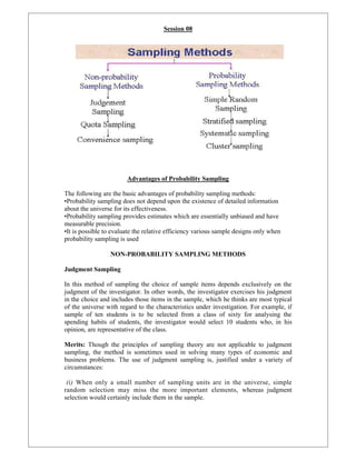
1. Session 08
Advantages of Probability Sampling
The following are the basic advantages of probability sampling methods:
•Probability sampling does not depend upon the existence of detailed information
about the universe for its effectiveness.
•Probability sampling provides estimates which are essentially unbiased and have
measurable precision.
•It is possible to evaluate the relative efficiency various sample designs only when
probability sampling is used
NON-PROBABILITY SAMPLING METHODS
Judgment Sampling
In this method of sampling the choice of sample items depends exclusively on the
judgment of the investigator. In other words, the investigator exercises his judgment
in the choice and includes those items in the sample, which he thinks are most typical
of the universe with regard to the characteristics under investigation. For example, if
sample of ten students is to be selected from a class of sixty for analysing the
spending habits of students, the investigator would select 10 students who, in his
opinion, are representative of the class.
Merits: Though the principles of sampling theory are not applicable to judgment
sampling, the method is sometimes used in solving many types of economic and
business problems. The use of judgment sampling is, justified under a variety of
circumstances:
(i) When only a small number of sampling units are in the universe, simple
random selection may miss the more important elements, whereas judgment
selection would certainly include them in the sample.

2. (ii) When we want to study some unknown traits of a population, some of whose
characteristics are known, we may then stratify the population according to these
known properties and select sampling units from each stratum on the basis of
judgment. This method is used to obtain a more representative sample.
(iii) In solving everyday business problems and making public policy decisions,
executives and public officials are often pressed for time and cannot wait for
probability sample designs. Judgment sampling is then the only practical method to
arrive at solutions to their urgent problems.
Limitations Judgment sampling method is however associated with the allowing
limitations:
(i) This method is not scientific because the population units to be sampled may be
affected by the personal prejudice or bias of the investigator. Thus, judgment
sampling involves the risk that the investigator may establish foregone conclusions by
including those items in the sample which conform to his preconceived notions. For
example, if an investigator holds the view that the wages of workers in a certain
establishment are very low, and if he adopts the judgment sampling method, he may
include only those workers in the sample whose wages are low and thereby establish
his point of view which may be far from the truth. Since an element of subjectiveness
is possible, this method cannot be recommended for general use.
(ii) There is no objective way of evaluating the reliability of sample results. The
success of this method depends upon the excellence in judgment. If the individual
making decisions is knowledgeable about the population and has good judgment, then
the resulting sample may be representative, otherwise the inferences based on the
sample may be erroneous. It may be noted that even if a judgment sample is
reasonably representative, there is no objective method for determining the size or
likelihood of sampling error. This is a big defect of the method.
Quota Sampling
Quota sampling is a type of judgment sampling and is perhaps the most commonly
used sampling technique in non-probability category. In a quota sample, quotas are set
up according to some specified characteristics such as so many in each of several
income groups, so, many in each age, so many with certain political or religious
affiliations, and so on. Each interviewer is then told to interview a certain number of
persons which constitute his quota. Within the quota, the selection of sample items
depends on personal judgment. For example, in a radio listening survey, the
interviewers may be told to interview 500 people living in a certain area and that out
of every 100 persons interviewed 60 are to be housewives, 25 farmers and 15 children
under the age of 15. Within these quotas the interviewer is free to select the people to
be interviewed. The cost per person interviewed may be relatively small for a quota
sample but there are numerous opportunities for bias which may invalidate
the results. For example, interviewers may miss farmers working in the fields or talk
with those housewives who are at home. If a person refuses to respond, the
interviewer simply selects someone else. Because of the risk of personal prejudice and
bias entering the process of selection, the quota sampling is not widely used in
practical work.
Quota sampling and stratified random sampling are similar in as much as in both
methods the universe is divided into parts and the total sample is allocated among the

3. parts. However, the two procedures diverge radically. In stratified random sampling
the sample with each stratum is chosen at random. In quota sampling, the sampling
within each cell is not done at random, the field representatives are given wide
latitude in the selection of respondents to meet their quotas.
Quota sampling is often used in public opinion studies. It occasionally provides
satisfactory results if the interviewers are carefully trained and if they follow their
instructions closely. It is often found that since the choice of respondents within a cell
is left to the field representatives, the more accessible and articulate people within a
cell will usually be the ones who are interviewed. Slight negligence on the part of
interviewers may lead to interviewing ineligible respondents. Even with alert and
conscientious field representatives it is often difficult to determine such control
category as age, income, educational qualifications, etc.
Convenience Sampling
A convenience sample is obtained by selecting 'convenient' population units. The
method of convenience sampling is also called the chunk A chunk refers to that
fraction of the population being investigated which is selected neither by probability
nor by judgment but by convenience. A sample obtained from readily available lists
such as automobile registrations; telephone directories, etc., is a convenience sample
and not a random sample even if the sample is drawn at random from the lists. If a
person is to submit a project report on labour-management relations in textile industry
and he takes a textile mill close to his office and interviews some people over there,
he is following the convenience sampling method. Convenience samples are prone to
bias by their very nature-selecting population elements which are convenient to
choose almost always make them special or different form the best of the elements in
the population in some way.
Hence the result obtained by following convenience sampling method can hardly be
representative of the population—they are generally biased and unsatisfactory.
However, convenience sampling is often used for making pilot studies. Questions
may be tested and preliminary information may be obtained by the chunk
before the final sampling design is decided upon.
PROBABILITY SAMPLING METHODS
Simple or Unrestricted Random Sampling
Simple random sampling refers to that sampling technique in which each and every
unit of the population has an equal opportunity of being selected in the sample. In
simple random sampling with items get selected in the sample is just a matter of
chance—personal bias of the investigator does not influence the selection. It should
be noted that the word 'random' does not mean "haphazard' or "hit-or-miss'—it rather
means that the selection process is such that chance only determines which items shall
be included in the sample. As pointed out by Chou, when a sample of size n is drawn
from a population with N elements, the sample is a 'simple random sample' if any of
the following is true. And, if any Of the following is true, so are the other two:
•All n items of the sample are selected independently of one another and all N items
in the population have the same chance of being included in the sample. By

4. independence of selection we mean that he selection of a particular item in one draw
has no influence on the probabilities of selection in any other draw.
•At each selection, all remaining items in the population have the same chance of
being drawn. If sampling is made with replacement, ie., when each unit drawn from
the population is returned prior to drawing the next unit, each item has a probability of
1/N of being drawn at each selection. If sampling is without replacement, i.e., when
each unit drawn from the population is not returned prior to drawing the next unit, the
probability of selection of each item remaining in the population at the first draw is
1/N, at the second draw is 1/(N-1), at the third draw is l/(N-2), and so on. It should be
noted that sampling with replacement has very limited and special use in statistics—
we are mostly concerned with sampling without replacement.
• All the possible samples of a given size n are equally likely to be selected. To
ensure randomness of selection one may adopt either the Lottery Method or consult
table of random numbers.
Lottery Method: This is a very popular method of taking a random sample. Under
this method, all items of the universe are numbered or named on separate slips of
paper of identical size and shape. These slips are then folded and mixed up in a
container or drum. A blindfold selection is then made of the number of slips required
to constitute the desired sample size. The selection of items thus depends entirely on
chance. The method would be quite clear with the help of an example. If we want to
take a sample of 10 persons out of a population of 100, the procedure is to write the
names of the 100 persons on separate slips of paper, fold these slips-mix them
thoroughly and then make a blindfold selection of 10 slips.
The above method is very popular in lottery draws where a decision about prizes is to
be made. However, while adopting lottery method it B absolutely essential to see that
the slips are of identical size, shape any colour, otherwise there is a lot of possibility
of personal prejudice an° bias affecting the results.
Table of Random Numbers: The lottery method discussed above become quite
cumbersome as the size of population increases. An alternative method of random
selection is that of using the table of random number
The random numbers are generally obtained by some mechanism which, when
repeated a large number of times, ensures approximately equal frequencies for the
numbers from 0 to 9 and also proper frequencies for various combinations
of number(such as 00,01,….999, etc) that could be expected in a random sequence of
the digits0 to 9.
Several standard tables of random numbers are available, among which the
following may be specially mentioned, as they have been tested extensively for
randomness:
* Tippett's (1927) random number tables consisting of 41,600 random digits grouped
into 10,400 sets of four-digit random numbers; .
* Fisher and Yates (1938) table of random numbers with 15,000 random
digits arranged into 1.500 sets of ten-digit random numbers;
* Kendall and Babington Smith (1939) table of random numbers
consisting of 1,00,000 random digits grouped into 25,000 sets of four-digit
random numbers; .
* Rand Corporation (1955) table of random numbers consisting of 1,00,000
random digits grouped into 20,000 sets of five-digit random numbers; and .
* C.R. Rao, Mitra and Mathai (1966) table of random numbers.

5. Tippett's table of random numbers is most popularly used in practice. We give below
the first forty sets from Tippett's table as an illustration of the general appearance of
random numbers:
2952 6641 3992 9792 7969 5911 3170 5624
4167 9524 1545 1396 7203 5356 1300 2693
2670 7483 3408 2762 3563 1089 6913 7991
0560 5246 1112 6107 6008 8125 4233 8776
2754 9143 1405 9025 7002 6111 8816 6446
It is important that the starting point in the table of random numbers be
selected in some random fashion so that every unit has an equal chance of
being selected.
One may question, and quite rightly, as to how it is ensured that these
digits are random. It may be pointed out that the digits in the table were chosen
haphazardly but the real guarantee of their randomness lies in practical tests.
Tippett's numbers have been subjected to numerous tests and used in many
investigations and their randomness has been well established for all practical
purposes. An example to illustrate how Tippett's table of random numbers
may be used is given below. Suppose we have to select 20 items out of 6,000.
The procedure is to number all the items from 1 to 6,000. A page from Tippett's
table may then be consulted and the first twenty numbers up to 6,000 noted
down. Items bearing those numbers will be included in the sample. Making use
of the Portion of the table given above the required numbers are:
2952 3992 5911 3170 5614 4167
1545 1396 5356 1300 26>3 2370
3408 2762 3563 1089 0550 5246
1112 4233
The items which bear the above numbers constitute the sample.
Universe size less than 1,000. If the size of universe is less than 1,000 the procedure
will be different, as Tippett's numbers are available only in four figures. Thus, for
example, if it is desired to take a sample of 10 items out of 400, all items from 1 to
400 should be numbered as 0001 to 0400. We may now select 10 numbers from the
table which are up to 0400.
Universe size less than 100. If the size of universe is less than 100, the table is used as
follows: Suppose ten numbers from out of 0 to 80 are required. We start anywhere in
the table and write down the numbers in pairs. The table can be read horizontally,
vertically, diagonally or in any methodical way. Starting with the first and reading
horizontally first (see table given above) we obtain 29, 52, 66, 41, 39, 92, 97, 92, 79,
69, 59, 11, 31, 70, 56, 24 70, 56, 24, 41, 67, and so on. Ignoring the numbers greater
than 80, we obtain for our purpose ten random numbers, namely, 29, 52, 66, .41, 39,
79, 69, 59, 11 and 31.
Fishers and Yate's tables consist of 15,000 numbers. These have been arranged in two
digits in 300 blocks, each block consisting of 5 rows and 5 columns. Kendall and
Smith also constructed random numbers (10,000 in all) by using a randomising

6. machine. However, this method of random selection cannot be followed in case of
articles like ghee, oil, petrol, wheat, etc.
Merits Simple random sampling method has the following advantages:
•Since the selection of items in the sample depends entirely on chance there is no
possibility of personal bias affecting the results.
•As compared to judgment sampling a random sample represents the universe in a
better way. As the size of the sample increases, it becomes increasingly
representative of the population.
•The analyst can easily assess the accuracy of this estimate because sampling errors
follow the principles of chance. The theory of random sampling is further developed
than that of any other type of sampling which enables the analyst to provide the most
reliable information at the least cost.
Limitations This method is however associated with following limitations:
•The use of simple random sampling necessitates a completely
catalogued universe from which to draw the sample. But it is often difficult for the
investigator to have up-to-date lists of all the items of the population to be sampled.
This restricts the use of this method in economic and business data where very often
we have to employ restricted random sampling designs.
•The size of the sample required to ensure statistical reliability is usually
larger under random sampling than stratified sampling.
•From the point of view of field survey it has been claimed that cases selected by
random sampling tend to be too widely dispersed Geographically and
that the time and cost of collecting data become.
• Random sampling may produce the most non-random looking results. For example,
thirteen cards from a well-shuffled pack of playing cards may consist of one suit. But
the probability of this type of occurrence is very, very low.
Restricted Random Sampling
1. Stratified Sampling Stratified random sampling or simply stratified sampling is one
of the random methods which, by using the available information concerning the
population, attempts to design a more efficient sample than obtained by the simple
random procedure.
While applying stratified random sampling technique, the procedure followed is given
below:
(a) The universe to be sampled is sub-divided (or stratified) into groups which are
mutually exclusive and include all items in the universe.
(b) A simple random sample is then chosen independently from each group.
This sampling procedure differs from simple random sampling in that in the latter the
sample items are chosen at random from the entire universe. In stratified random
sampling the sampling is designed so that a designated number of items is chosen
from each stratum. In simple random sampling the distribution of the sample among
strata is left entirely to chance.
How to Select Stratified Random Sample?
Some of the issues involved in setting up a stratified random sample are :

7. (i) Base of Stratification What characteristic should be used to sub divide the universe
into different strata? As a general rule, strata are created on the basis of a variable
known to be correlated with the variable of interest and for which information on each
universe element is known. Strata should be constructed in a way which will
minimize differences among sampling units within strata, and maximize difference
among strata.
For example, if we are interested in studying the consumption pattern °f the people of
Delhi, the city of Delhi may be divided into various parts (such as zones or wards)
and from each part a sample may be taken at random. Before deciding on
stratification we must have knowledge of the traits of the population. Such knowledge
may be based upon expert Judgment, past data, preliminary observations from pilot
studies, etc.
The purpose of stratification is to increase the efficiency of sampling by dividing a
heterogeneous universe in such a way that Q there is as great a homogeneity as
possible within each stratum, and (ii) a marked difference is possible between the
strata.
(ii) Number of Strata. How many strata should be constructed? The Practical
considerations limit the number of strata that is feasible, costs of adding more strata
may soon outrun benefits. As a generalization more than six strata may be
undesirable.
(iii) Sample size within Strata How many observations should be taken from each
stratum? When deciding this question we can use either a proportional or a
disproportional allocation. In proportional allocation, one samples each stratum in
proportion to its relative weight. In disproportional allocation this is not the case. It
may be pointed out that proportional allocation approach is simple and if all one
knows about each stratum is the number of items in that stratum, it is generally also
the preferred procedure. In disproportional sampling, the different strata are sampled
at different rates. As a general rule when variability among observations within a
stratum is high, one samples that stratum at a higher rate than for strata with less
internal variation.
Proportional and Disproportional Stratified Sample
In a proportional stratified sampling plan, the number of items drawn from each strata
is proportional to the size of the strata. For example, if the population is divided into
five groups, their respective sizes being 10, 15, 20, 30 and 25 per cent of the
population and a sample of 5,000 is drawn, the desired proportional sample may be
obtained in the following manner:
From stratum one 5,000 (0.10) = 500 items
From stratum two 5,000(0.15) = 750 items
From stratum three 5,000 (0.20) = 1,000 items
From stratum four 5,000 (0.30) = 1,500 items
From stratum five 5,000(0.25) = 1,250 items
Total = 5,000 items
Proportional stratification yields a sample that represents the universe with respect to
the proportion in each stratum in the population. This procedure is satisfactory if there
is no great difference in dispersion from stratum to stratum. But it is certainly not the
most efficient procedure, especially when there is considerable variation in different
strata. This indicates that in order to obtain maximum efficiency in stratification,, we

8. should assign greater representation to a stratum with a large dispersion and smaller
representation to one with small variation.
In disproportional stratified sampling an equal number of cases is taken from each
stratum regardless of how the stratum is represented in the universe. Thus, in the
above example, an equal number of items (1,000) from each stratum may be drawn.
In practice disproportional sampling is common when sampling forms a highly
variable universe,, wherein the variation of the measurements differs greatly from
stratum to stratum.
Merits Stratified sampling methods have the following advantages:
• More representative. Since the population is first divided into various strata
and then a sample is drawn from each stratum there is a little possibility of any
essential group of the population being completely excluded. A more
representative sample is thus secured. C.J. Grohmann has rightly pointed
out that this type of sampling balances the uncertainty of random
sampling against the bias of deliberate selection.
• Greater accuracy. Stratified sampling ensures greater accuracy. The accuracy is
maximum if each stratum is so formed that it consists of uniform or homogeneous
items.
• Greater geographical concentration. As compared with random sample, stratified
samples can be more concentrated geographically, i.e., the units from the different
strata may be selected in such a way that all of them are localised in one
geographical area. This would greatly reduce the time and expenses of interviewing.
Limitations The limitations of this method are:
• Utmost care must be exercised in dividing the population into various strata. Each
stratum must contain, as far as possible, homogeneous items as otherwise the
results may not be reliable. If proper stratification of the population is not done, the
sample may have the effect of bias.
• The items from each stratum should be selected at random. But this may be
difficult to achieve in the absence of skilled sampling supervisors and a random
selection within each stratum may not be ensured.
• Because of the likelihood that a stratified sample will be more widely distributed
geographically than a simple random sample cost per observation may be
quite high.
2. Systematic Sampling: A systematic sample is formed by selecting one unit at
random and then selecting additional units at evenly spaced intervals until the sample
has been formed. This method is popularly used in those cases where a complete list
of the population from which sample is to be drawn is available. The list may be
prepared in alphabetical, geographical, numerical or some other order. The items are
serially numbered. The first item is selected at random generally by following the
Lottery method. Subsequent items are selected by taking every kth item from the list
where 'k refers to the sampling interval or sampling ratio, i.e., the ratio of population
size to the size of the sample. Symbolically:
N
n
k 
where k = Sampling interval, N = Universe size, and n = Sample size.

9. While calculating k, it is possible that we get a fractional value. In such a case we
should use approximation procedure, le., if the fraction is less than 0.5 it should be
omitted and if it is more than 0.5 it should be taken as 1. If it is exactly 0.5 it should
be omitted, if the number is even and should be taken as 1, if the number is odd. This
is based on the principle that the number after approximation should preferably be
even. For example, if the number of students is respectively 1,020, 1,150 and 1,100
and we want to take a sample of 200, k shall be:
1020
(i) 5.1 5
k   or
200
1150
k   or
(ii) 5.75 6
200
1100
k   or
(iii) 5.5 6
200
Merits : The systematic sampling design is simple and convenient to adopt.
The time and work involved in sampling by this method are "relatively
less. The results obtained are also found to be generally satisfactory
provided care is taken to see that there are no periodic features
associated with the sampling interval. If populations are sufficiently
large, systematic sampling can often be expected to yield -suits similar to
those obtained by proportional stratified sampling.
Limitations: The main limitation of the method is that it become less representative if
we are dealing with populations having “hidden periodicities”. Also if the population
is order in a systematic way with respect to the characteristics the investigator is
interested in , then it is possible that only certain types of item will be included in the
population, or at least more of certain types than others. For instance, in a study of
worker’ wages the list may be such that every tenth worker on the list gets wages
above Rs. 750per month.
3. Multi-stage Sampling or Cluster Sampling: Under this method the random selection
is made of primary, intermediate and final ( or the ultimate) units from a given
population or stratum. There are several stages in which the sampling process is
carried out. At first, he first stage units are sampled by some suitable method, such as
sample random sampling. Then, a sample of second stage units is selected from each
of the selected first stage units, again by some suitable method which may be the
same as or different from the method employed for the first stage units. Further stages
may be added as required.
Merits Multi-stage sampling introduces flexibility in the sampling method which is
lacking in the other methods. It enables existing divisions and sub-divisions of the
population to be used as units at and permits the field work to be concentrated and
yet large area to be covered. Another advantage of the method is that subdivision into
second stage units (i.e., the construction of the second stage frame) need be
carried out for only those first stage units which are included in the sample. It is,
therefore, particularly valuable in surveys of underdeveloped areas where no
frame is generally sufficiently detailed and accurate for subdivision of the
material into reasonably small sampling units.

10. Limitations: However, a multi-stage sample is in general less than a sample
containing the same number of final stage units which have been selected by some
single stage process.
We have discussed above the various random procedures in independent
designs. In practice we often combine two or more of these methods into a single
design.
SAMPLING DISTRIBUTION AND STANDARD ERROR
Suppose a sample of size n is drawn from a population and the sample mean x is
calculated. From the population, many such sample of the same size can be drawn.
For each of these samples, x can be calculated. And so, there can be many values of
x Suppose these different values of x are tabulated in the form of a frequency
distribution, the resulting distribution is called Sampling distribution of x The
standard deviation of this sampling distribution is called Standard Error (S.E)
The distribution of values of a statistic for different samples of the same size is
called sampling distribution of the statistic.
Standard Error (S.E.) of a statistic is the standard deviation of the sampling
distribution of the statistic.
Sampling distributions of other statistics such as sample variance, sample median,
etc., can also be written down. In each of these case, the corresponding standard
deviation would be the standard error (SE).
Consider a population whose means is μ and standard deviation σ. Let a random
sample of size n be drawn from this population. Then, the sampling distribution of x
has mean μ and standard error
 . That is, E( x ) = μ and S.E.( x ) =
n
n

Let a random sample of size n1 be drawn from population whose mean is μ1 and
σ1 standard deviation. And also, let a random sample of size n2 be drawn from another
population whose mean is μ2 and standard deviation is σ2 . Let x 1 be the mean of the
first sample and x 2 be the mean of the second sample . Then,
2
2
2
2
1
1
( 1 2 ) ( 1 2 ) . .(( 1 2 ))
n n
E x x andS E x x
 
       
STATISTICAL HYPOTHESIS
A statistical hypothesis is an assertion regarding the statistical distribution of the
population. It is a statement regarding the parameters of the population
Statistical hypothesis is denoted by H
Examples:
1. H: The population has mean μ = 25
2. H: The population is normally distributed with mean μ=25 and standard deviation
In a test procedure, to start with, a hypothesis is made. The validity of this hypothesis
is tested. If the hypothesis is found to be true, it is accepted. On the other hand, if it is
found to be untrue, it is rejected

11. The hypothesis which is being tested for possible rejection is called null
hypothesis. The null hypothesis is denoted by H0. Hypothesis which is accepted when
the null hypothesis is rejected is called alternative hypothesis The alternative
hypothesis is denoted by H1.
CRITICAL REGION
From a population many samples of the same size n can be drawn. Let S be the set of
all such sample of size n that can be drawn from the population. Then, S is called
sample space. While testing a null hypothesis, among the samples which belong to S,
some samples lead to the acceptance of the null hypothesis, whereas, some others lead
to the rejection of the null hypothesis. The set of all those samples belonging to the
sample space which lead to the rejection of the null hypothesis is called critical
region. The critical region ids denoted by ω. The critical region is also rejection
region. The set of samples which lead to the acceptance of the null hypothesis is the
acceptance region. It is (S- ω).
In fact, to decide whether the sample in hand belongs to ω, the criterian |Z| > k is
adopted. And so, in effect, the critical region is defined by |Z| >ks.
ERRORS OF THE FIRST AND THE SECOND KIND
Type I and type II errors)
While testing a null hypothesis against an alternative hypothesis, one f the following
four situations arise
Actual fact Decision based on the
sample
Error
1 H0 is true accept H0 correct decision -
2 H0 is true reject H0 wrong decision Type I
3 H0 is not true accept H0 wrong decision Type II
4 H0 is not true reject H0 correct decision -
Here, in situations (2) and (3), wrong decisions are arrived at. These wrong decisions
are Error of the first kind (Type I error) and Error of the second kind (Type II error)
respectively. Thus,
(i) Error of the first kind (Type I error) is taking a wrong decision to reject the
null hypothesis when it is actually true.
(ii) Error of the second kind (Type II error) is taking a wrong decision to
accept the null hypothesis when it is actually not true.

12. The probability of occurrence of the first kind of error is denoted by α. It is called
level of significance. Thus, the level of significance is the probability of Type I
error. It is the probability of rejection of the null hypothesis when it is actually
true. Usually the level of significance is fixed at 0.05 or 0.01. In other words, the
level is fixed at 5% or 1%.
The probability of occurrence of the second kind of error is denoted by β.
The value (1- β) is called power of the test. Power of a test is the probability of
rejecting H0when it is not true.
While testing, the level of significance α is decided in advance. Then, the critical
value k is determined in such a way that the power (1- β) is maximum.
Thus, the critical value k is based on the level of significance. For tests which are
based on normal distribution, if α=0.05, the critical value is k = 1.96. If α=0.01, the
critical value is k = 2.58.
Note: In fact, a decision to accepts H0, is based only on the given data. And so,
rather than making an assertive statement ‘H0 is accepted’, we would make a
statement ‘H0 is not rejected’. However, at the level of this book, we will not
bother about the subtle difference between these statements
TWO-TAILED AND ONE-TAILED TESTS (Two-sided and one-sided testes)
While testing H0, if the critical region is considered at one tail of the sampling
distribution of the test statistic, the test is one-tailed test
One the other hand, if the critical region is considered at both
the tails of the sampling distribution of the test statistic,
the test is two-tailed test.