1. Tools for applied trade-policy analysis :
An introduction
Soamiely Andriamananjara
Olivier Cadot
Jean-Marie Grether
Revised version
July 2010
Abstract
This paper provides a non-technical introduction to some of the issues faced by a
beginner trade-policy analyst: where to find data, how to calculate descriptive indices,
what are the practical difficulties involved in measurement and calculation, how to
perform simple statistical analyses of the effect of trade policies on domestic incomes,
and how to approach ex-ante simulation analysis. Throughout the paper, we keep the
level of exposition at a level that is accessible to a reader trained in economics but with
limited proficiency in formal theory and econometrics. The last part of the paper, which
describes Computable General Equilibrium (CGE) analysis, is not meant to enable the
reader to perform such analysis but rather to read existing simulation results and
understand what to look for.
1

2. 1. Introduction
Not so long ago, the analysis of trade policy required not just a sound knowledge
of theory and analytical tools, but also familiarity with cranky software and a
willingness to replace missing data with heroic assumptions. The picture has
changed drastically over the last quarter-century. The availability and quality of
trade statistics has improved under the combined effort of researchers and
statisticians at UNCTAD, the World Bank, and others institutions. Software has
also become more user-friendly, making the calculation of complex indices easy
even with minimal computing skills.
Thus, there is no excuse anymore for staying away from formal analysis, whether
it be calculating descriptive indices or estimating statistical relationships. This
paper presents a palette of tools which, taken together, enable the analyst to
produce a rigorous yet “readable” picture of the policy-relevant features of a
country’s trade and of the consequences of trade-policy choices. All these tools
have been proposed and explained in the literature. For instance, Michaely
(1996), Yeats (1997), Brulhart (2002), Hummels and Klenow (2005), Hausmann,
Hwang, and Rodrik (2005), Shihotori, Tumurchudur and Cadot (2010), or Cadot,
Carrère and Strauss-Kahn (forthcoming) discussed the indices presented in
Section 2 of this paper. Kee et al. (2004, 2006) discuss in detail the construction of
trade restrictiveness indices discussed in section 3. The gravity equation has been
discussed in too many papers and contexts to be counted here. The collection of
essays in Francois and Reinert (1997) give a thorough analytical discussion of the
ex-ante simulation tools presented in Section 4, and Jammes and Olarreaga (2006)
discuss the World Bank’s SMART model. But most of these readings remain
difficult and leave a gap between the needs of a theoretical or classroom
discussion and those of the practitioner.
This paper intends to fill some of this gap by discussing practical data and
implementation issues for the most widely used among those tools. Starting with
the simplest descriptive methods, we will move progressively to more analytical
ones, but always keeping the exposition at a level comprehensible to the non-
academic practitioner. The last part of the paper, devoted to ex-ante simulation
analysis (in partial and general equilibrium), however, remains difficult. The
construction of simulation models requires advanced mastery of both economic
theory and appropriate programming languages such as GAMS and remains
largely beyond the capability of the beginning analyst, although specialized
training programs are regularly given around the world. The models are
inherently complex and sensitive to assumptions, making mistakes and
misinterpretations easy. Thus, our aim in that part of the paper is limited:
essentially, to enable the reader to get a feel for how these models are
2

3. constructed, and to be in a better position to understand what can be asked from
those models and what cannot.
Given the space limitations of a survey paper, there is necessarily a trade-off
between depth and breadth. We have chosen to err on the “depth” side, not by
going into deep discussions of the underlying concepts −those can be found in
the original papers and in standard trade textbooks− but rather by discussing
practical implementation issues of relevance to the novice practitioner. The price
to pay for this is that we had to limit the number of indices and approaches we
cover.
The paper is organized as follows. Section 2 discusses how to present a
panorama of a country’s trade performance, and how to present standard
measures of its trade-policy stance. Section 3 presents some of the econometric
techniques that can be used to assess, ex post, the effect of trade policies on trade
flows and the domestic economy. Section 4 presents some of the tools used in the
ex-ante assessment of trade policy, first in partial equilibrium settings, then in
general-equilibrium ones. Section 5 concludes.
2. Analyzing trade flows & policy: descriptive tools
2.1 Trade flows
2.1.1. Data
The first issue the analyst must deal with is the data. What database is
appropriate depends on whether the analysis is to be performed at the
aggregated (total) level or at the disaggregated one (by commodity). In the
former case, the IMF’s Direction of Trade Statistics (DOTS) is the right source. In
the latter case, it should be UNCTAD’s COMTRADE database. COMTRADE is
much more voluminous than the DOTS because it contains data on bilateral
trade between all countries in the UN system for over 5’000 commodities.1
Next, if dealing with disaggregated data, the analyst must choose between
several classification systems. First and foremost is the Harmonized System (HS)
in which all countries report their trade data to COMTRADE. Under revision in
2007, the HS system has four levels: 21 sections, 99 chapters (also called “HS2”
1
The DOTS are available on CD ROM by subscription for a moderate price.
COMTRADE is available only online, either through the World Bank’s WITS gateway or
directly, but in any case by subscription, for a price that is considerably higher than the
DOTS.
3

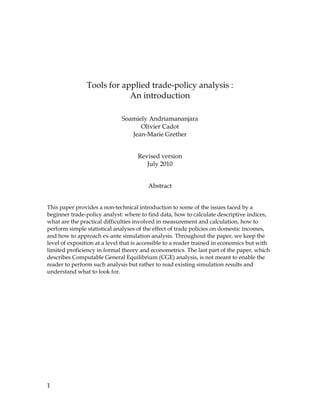
4. because chapters are coded in two-digit codes from 01 to 99), 1’243 headings
(HS4) and 5’052 sub-headings (HS6). More disaggregated levels (HS8 and HS10)
are not harmonized and need considerable cleaning up before use.2 As is well
known, at high levels of disaggregation (in particular HS6), the HS system has
the peculiarity that it is very detailed for some sectors like textile and clothing,
but much less so for others like machinery. As a result, the economic importance
of subheadings can very considerably and care should be exercised when using
simple averages (more below). However this oft-mentioned bias should not be
overstated: as Figure 1 shows, the share of each HS section in the total number of
HS6 lines is highly correlated with its share in world trade.
Figure 1
HS sections shares in HS6 lines and in world trade
16
.3
Share of export value in total export
.2
17
.1
6
15 11
5
718
100 4
2
1 2
14 9 13
12
8
19 3
0
0 .05 .1 .15 .2
Share of export number of lines in total export
Notes: 131 countries, average 1988-2004. Section 11 is textile & apparel, section 16 is
machinery, section 17 is transport equipment.
The main alternative classification system is the SITC Rev. 4 (adopted in 2006)
which has 5 levels of disaggregation, also by increasing number of digits.
Although SITC subgroups (4 digits) number about as many (1’023) as HS4
headings, they don’t match perfectly, so concordance tables must be used (see
Annex II.5 of United Nations 2006). Whether the HS or the SITC should be used
is largely governed by the type of data to which raw trade numbers are to be
matched in the analysis. If it is confined to pure trade analysis, the choice is
inconsequential. More importantly, a number of classifications exist in which
goods are classified under different logics. For instance, the UN has devised
“Broad Economic Categories” (BEC) by end use: capital goods (01), raw materials
2
For the EU, Eurostats provides HS 8 data on its COMEXT CD ROM, but frequent
reclassifications require considerable caution in use. HS 10 data is available only
internally. For the US, the NBER provides a clean HS 10 database compiled by Robert
Feenstra and updated by Feenstra, John Romalis and Jeffrey Schott.
4

5. (02), semi-finished goods (03), and final ones (04). This classification is useful for
instance to assess “tariff escalation” (higher tariffs on final goods than on other
categories, a practice that is used to protect domestic downstream transformation
activities and is frequent in developing countries). James Rauch devised a
alternative classification of goods according to their degree of differentiation,
from homogenous to reference-priced to fully differentiated.3 The former uses
HS codes, the latter SITC ones. Rauch’s classification is useful for many
purposes; for instance, competition is likely to take different forms on
homogenous vs. differentiated-good markets (price-based for the first, quality,
service or technology-based for the second).
2.1.2 Measurement
One might think that trade flows are about the easiest thing to measure since
merchandises must be cleared at customs. Unfortunately, the statistics that
measure them are surprisingly erratic. Country A’s measured imports from B
seldom match B’s measured exports to A, and the latter are typically reported
with large errors because customs do not monitor exports very closely. Thus,
whenever possible partner import data should be used in lieu of direct export
data, a technique called “mirroring”. Sometimes, however, and in particular for
poor countries, even import data are very erratic, in which case mirroring should
be used using export data from source countries. Figure 2, which shows
Zambia’s mirrored against direct import data at the HS6 level, illustrates the
problem. Although the two are clearly correlated, the dispersion around the
diagonal (along which they are equal, as they should be) is substantial.
Moreover, direct data is not systematically under-estimated compared to mirror
data: the bias seems to go either way.
Figure 2
Zambia’s mirrored imports against direct data
3
Details on the BEC classification can be found in UN (2003). Rauch’s classification can
be found on Jon Haveman and Raymond Robertson’s web page.
5

6. Zambia's stats (log scale) diagonal
18
16
14
12
10
8
6
4
2
0
0 2 4 6 8 10 12 14 16 18
mirrored stats (log scale)
Source : Cadot et al. 2006a
Note: truncation point along horizontal axis equal to US$403’000; no partner indications
for annual trade values below that threshold.
Discrepancies between importer and exporter data are reconciled in BACI, a
database put together by the CEPII in Paris. However BACI trails COMTRADE
with an approximate two-year lag.
In addition to trade values, COMTRADE reports trade volumes (in tons, units,
etc.) from which unit values can be recovered by dividing values by volumes.
Unit values can be useful e.g. to convert specific tariffs into ad-valorem ones.
They are however very erratic because volumes, which are measured less
precisely than values, are in the denominator. When they are under-reported by
mistake, unit values can become absurdly large. In addition, unit values vary
−and should vary− across countries because of composition problems. Schott
(2004) showed that they are correlated with the exporter’s GDP per capita, as
goods exported by richer countries are likely to embody higher quality or
technology even if classified under the same heading as those exported by poorer
countries. They should therefore be used very cautiously.
2.2 Trade composition
The sectoral composition of a country’s trade should be in the TS for two reasons.
First, it may matter for growth if some sectors are growth drivers, although
whether this is true or not is controversial.4 Second, constraints to growth may be
more easily identified at the sectoral level.5 The geographical composition
4
5
See Hausmann, Hwang and Rodrik 2005.
On this, see McKinsey Global Institute 2010.
6

7. highlights linkages to dynamic regions of the world (or the absence thereof) and
helps to think about export-promotion interventions. It is also a useful input in
the analysis of regional integration, an item of rising importance in national trade
policies.
The simplest way of portraying the sectoral orientation of a country’s exports is
in the form of a “radar screen”, as in Figure 1. When displaying a graph of that
type, sectoral aggregates have to be selected carefully (more detail in the
categories that matter for that country), and so has to be the scale. When one
sector/product hugely dominates the picture, it will be more readable on a log
scale. Log transformations are often useful to prevent outliers from obfuscating
the picture.
Figure 1
Sectoral orientation of Nepal’s exports
The geographical composition can be shown the same way, with the same
scaling issues, or in percentages, as in Figure 2. Notice the drastic re-orientation
of Nepal’s exports toward India. This calls for an explanation, which we
postpone to Section 3.
Figure 2
Geographical orientation of Nepal’s exports, 1998 and 2008
One can go a step further and assess, with a simple graph, to what extent outside
demand-pull factors affect domestic trade performance. Consider the
geographical version of the thing; the sectoral version goes the same way. Take
all destination countries for home exports; calculate their share in total home
exports, call it x, and put it in logs.6 Next, record the growth rate of total imports
6
Logs will be negative because shares are less than one. That is not a problem.
7

8. for each of those countries over the last ten years; call it y. Do a scatterplot of y
against log(x) and draw the regression line. If it slopes up, larger destinations
have faster import growth; the orientation is favorable. If it slopes down, as in
Figure 3, larger destinations (to the right of the picture) have slower import
growth; the orientation is unfavorable. In the latter case, the story may e.g. reflect
a mixture of the country’s location and policy choices; in Pakistan’s case,
proximity to slow-growing Gulf and Central Asian states combined with failure
to promote trade integration with fast-growing India to produce a negative
orientation.
Figure 3
Geographical orientation of Pakistan’s exports
Growth Orientation of Pakistan's Destinations, 2008
Log of Import Growth of Countries (2000-08)
6.5
6
5.5
5
4.5
4
-2 -1 0 1 2 3
Log of Destination's Share in Exports (%)
A similar scatterplot can be constructed using product shares in home export and
the rate of growth of world trade in those products, or, even better, product-
destination shares. A negative correlation, indicating positioning on slow-
growing products, may provide a useful factual basis for discussions about
whether Government resources should be used to foster growth at the extensive
margin (e.g. through sector-specific fiscal incentives).
When one is interested in the convergence of trade and production patterns
between a developing (“Southern”) country and “Northern” trade partners, a
useful indicator is Grubel and Lloyd’s intra-industry trade index,
X kij − M kij
GL = 1 −
ij
X kij + M kij
k
where, as usual X kij is i’s exports to j of good k and the bars denote absolute
values. The standard interpretation of the GL index, which runs between zero
(for inter-industry trade) to one (for intra-industry trade). High values of the GL
index are consistent with the type of trade analyzed in, say, Krugman’s
monopolistic-competition model. For a developing country’s trade with an
8

9. industrial country, rising values are therefore typically associated with
convergence in income levels and industrial structures.7
However GL indices should be interpreted cautiously. First, they rise with
aggregation (i.e. they are lower when calculated at more detailed levels), so
comparisons require calculations at similar levels of aggregation. More
problematic, unless calculated at extremely fine degrees of disaggregation, GL
indices can pick up “vertical trade”, a phenomenon that has little to do with
convergence and monopolistic competition. If, say, Germany export car parts
(powertrains, gearboxes, braking modules) to the Czech Republic which then
exports assembled cars to Germany, a GL index calculated at an aggregate level
will report lots of intra-industry trade in the automobile sector between the two
countries; but this is really “Heckscher-Ohlin trade” driven by lower labor costs
in the Czech Republic (assembly is more labor-intensive than component
manufacturing, so according to comparative advantage it should be located in
the Czech Republic rather than Germany).
2.3 Margins of expansion/diversification
Export Diversification, in terms of either products or destinations, can be at the
intensive margin (a more evenly spread portfolio) or at the extensive margin
(more export items). Diversification is measured (inversely) by indices like
Herfindahl’s concentration index (the sum of the squares of the shares) or Theil’s
(more complicated but pre-programmed in Stata). If the indices are calculated
over active export lines only, they measure concentration/diversification at the
intensive margin. Diversification at the extensive margin can be measured
simply by counting the number of active export lines. The first thing to observe is
that, in general, diversification at both the intensive and extensive margins goes
with economic development, although rich countries re-concentrate (see Figure
4).
Figure 4
Export concentration and stages of development
7
In this regard one may prefer to use marginal IIT indices, discussed in Brülhart (2002).
9

10. 5000
7
# active export lines
1000 2000 3000 4000
number of exported products
6
Theil index
5
Theil index
4
0
3
0 20000 40000 60000
GDP per capita PPP (constant 2005 international $)
Active lines - quadratic Active lines - non parametric
Theil index - non parametric Theil index - quadratic
Source: Cadot, Carrere and Strauss-Kahn (forthcoming).
Whether diversification is a policy objective in itself is another matter. Sometimes
big export breakthroughs can raise concentration, as semiconductors did for
Costa Rica. Diversification is also often justified to avoid the so-called “natural
resource curse” (a negative correlation between growth and the importance of
natural resources in exports), but whether the curse is real or a statistical illusion
has recently become a matter of controversy. 8 So one should be careful in taking
diversification as a policy objective per se. What is clear is that, in principle,
diversification reduces risk, although the concept of “export riskiness” has been
relatively unexplored.9 In addition, diversification at the extensive margin
reflects “export entrepreneurship” and, in that sense, is useful evidence on the
business climate.
One drawback of measuring diversification by just counting active export lines
(as in Figure 4) is that whether you diversify by starting to export crude
petroleum or mules, asses & hinnies is the same: you add one export line (at a
given level of product disaggregation). Hummels and Klenow (2005) have
proposed a variant where new export lines are weighted by their share in world
trade. Then, starting to export a million dollars worth of crude counts more than
starting to export a million dollar worth of asses, because the former is more
important in world trade (and therefore represents a stronger expansion
potential).
8
On export breakthroughs raising concentration, see Easterly, Resheff & Schwenkenberg
(2009). On the natural-resource curse, see e.g. Brunnschweiler and Bulte (2009) and the
contributions in Lederman and Maloney (2009).
9
The World Bank is working on a concept of “export riskiness” for foodstuffs, using
econometric analysis of counts of sanitary alerts at the E.U. and U.S. borders. Di
Giovanni and Levchenko (2010) propose a more general measure of riskiness based on
the variance-covariance matrix of sectoral value added.
10

11. Let Ki be the set of products exported by country i, the dollar value of i’s
exports of product k to the world, and the dollar value of world exports of
product k. The (static) intensive margin is defined by HK as
In words, the numerator is i’s exports and the denominator is world exports of
products that are in i’s export portfolio. That is, IMi is i’s market share in what it
exports. The extensive margin (also static) is
where Kw is the set of all traded goods. XMi measures the share of the products
belonging to i’s portfolio in world trade. Both measures are illustrated in Figure
5.
Figure 5
Evolution of intensive and extensive margins, Pakistan and Costa Rica
Your market
share in your
export portfolio
Intensive and Extensive Margin in Products, 1993-03
Big fish in a small
.2
pond Pakistan
.12 .14 .16 .18
Intensive Margin
Costa Rica
Pakistan
Costa Rica Small fish in
.1
a big pond
84 86 88 90 92 94
Extensive Margin Weight of your
1993 2003 export portfolio
in world trade
For Pakistan, the picture shows that its export portfolio was broadening during
the period, but that existing exporters failed to maintain market share.
As for Costa Rica, it managed to diversify at both the intensive and extensive
margins after Intel’s investment in 1996. This may seem surprising—one would
have expected the country to move from big fish in the (relatively) small pond of
banana exporters to small fish in the larger pond of semiconductor exporters. Yet
it became “bigger fish in a bigger pond”. The reason for this paradox is simple:
Costa Rica was already exporting semiconductors, albeit in very small quantities,
11

12. before Intel. This highlights another golden rule: Always look at the raw
numbers, not just indicators. It is very easy to get puzzled or misled by
indicators, and the more complicated the trickier.
Export expansion can also be defined at the intensive margin (growth in the
value of existing exports), at the extensive margin (new export items, new
destinations) or at the “sustainability margin” (longer survival of export spells).
A useful decomposition goes as follows. Using notation already introduced, let
base-year exports be
and terminal exports
The variation in total export value between those two years can be decomposed
into
where the first term is export variation at the intensive margin, the second is the
new-product margin, and the third is the “product death margin”. In words,
export growth can be boosted by exporting more of existing products, by more
new products, or by fewer failures. Note that the new-product margin, which is
conceptually equivalent to the extensive margin, is measured here by the dollar
value of new exports, not by their number.
More complicated decompositions can be constructed, along the same lines,
combining products and destinations. One useful fact to know is that the
contribution of the new-product margin to export growth is generally small
(Figure 6).
Figure 6
Decomposition of the export growth of 99 developing countries, 1995-2004
12

13. Expanding export relationships
New destinations, existing products
New products, existing destinations
New products to new destinations
Death of export relationships
Shrinking export relationships
-40 -20 0 20 40 60 80 100 120
Source: Brenton and Newfarmer (2009).
There are two reasons for that, one technical and one substantive. The technical
one is that a product appears in the extensive margin only the first year it is
exported; thereafter, it is in the intensive margin. So unless you start exporting
on a huge scale the first year (unlikely) the extensive margin’s contribution to
overall export growth can only be small. The substantive reason is that most new
exports fail shortly after they have been launched: median export spell length is
about two years for developing countries. There is a lot of export
entrepreneurship out there, but there is also a lot of churning in and out. Raising
the sustainability of exports (which requires an understanding of the reasons for
their low survival) is one under-explored margin of trade support.10
2.4 Export-expansion potential
Suppose that it is easier for a producer to expand into new markets with existing
products than to start exporting new products. Based on this idea, Brenton and
Newfarmer (2009) proposed an index of export market penetration defined, at
the product level, as the share of potential destination markets that the country
actually reaches (i.e. the ratio of the number of i’s destination countries for
product k relative to the number of countries importing product k from
anywhere). This type of information is useful background for trade-promotion
interventions.
When the issue is regional export-expansion potential (e.g. to be expected from a
preferential agreement) one useful index is Michaely’s bilateral trade-
complementarity index (Michaely 1996). Intuitively, it is best thought of as a
correlation between country A’s exports to the world with country B’s imports
10
The World Bank is currently exploring the causes of Africa’s low export survival.
Surveys highlight the unavailability of credit as a key binding constraint not just to
export entrepreneurship but to the survival of existing export relationships.
13

14. from the world. A is likely to have a comparative advantage in products it exports
a lot to the world (i.e. without the help of tariff preferences); if those products are
those in which B has a comparative dis-advantage (because it imports a lot of it),
well then A and B should marry.
Formally, the TCI is not a statistical correlation but an (algebraic) indicator. Let
be product k’s share in A’s imports from the world and its share in B’s
exports to the world; both should be at the HS6 level of disaggregation. The
formula is
and can easily be calculated in excel. The higher the index, the higher the scope
for non-diversion (efficient) trade expansion between A and B. Note that there
are two indices for each country pair, one taking A as exporter and one taking it
as importer. Sometimes the two indices are quite different. The country in a bloc
whose import pattern fits with its partners’ exports will act as a trade engine for
the bloc; the one whose export pattern fits with its partners’ imports will benefit
(in political-economy terms) from the agreement.
Table 1 shows two illustrative configurations with three goods. In panel (a), i’s
offer does not match j’s demand as revealed by their exports and imports
respectively. Note that these exports and imports are by commodity but to the
world, not to each other.
Table 1
Trade complementarity indices
Dollar amount of trade
country i country j
goods X ki i
Mk Xkj Mkj
1 0 55 108 93
2 0 0 0 0
3 23 221 35 0
Total 23 276 143 93
Shares in each country's trade Intermediate calculations
country i country j Cross differences Absolute values
goods i
xk
i
mk xkj mkj mkj − xk
i
mk − xkj
i
mk − xkj / 2
i
mkj − xk / 2
i
1 0.00 0.20 0.76 1.00 1.00 -0.56 0.50 0.28
2 0.00 0.00 0.00 0.00 0.00 0.00 0.00 0.00
3 1.00 0.80 0.24 0.00 -1.00 0.56 0.50 0.28
sum 1.00 1.00 1.00 1.00 0.00 0.00 1.00 0.56
Index value 0.00 44.40
14

15. 2.5 Comparative advantage
The current resurgence of interest for industrial policy sometimes confronts trade
economists with demands that they are loath to respond to—providing guidance
to pick winners. In general, there is little to rely on to predict the viability of an
infant industry, beyond comparative advantage. But even identifying
comparative advantage is tricky. The traditional measure is Balassa’s Revealed
Comparative Advantage (RCA) index, a ratio of product k’s share in country i’s
exports to its share in world trade. Formally,
X ki / X i
RCAki =
Xk / X
where X ki is country i's exports of good k, X i = ∑k X ki its total exports,
X k = ∑i X ki world exports of good k and X = ∑i ∑k X ki total world exports. An
RCA over one in good (or sector) k for country i means that i has a revealed
comparative advantage in that sector. RCA indices are very simple to calculate
from COMTRADE and can be calculated at any degree of disaggregation. But
Balassa’s index simply records country i’s current trade pattern; it cannot be used
to say whether or not it would make sense to support a particular sector.
An alternative approach draws on the PRODY index developed by Hausmann,
Hwang and Rodrik (2005). The PRODY approximates the “revealed” technology
content of a product by a weighted average of the GDP per capita of the
countries that export it, where the weights are the exporters’ RCA indices for that
product (adjusted to sum up to one). Intuitively, a product exported by high-
income countries is likely to be more technology intensive than one exported by
low-income countries. A recent database constructed by UNCTAD extends that
notion to revealed factor intensities. Let ki = Ki/Li be country i’s stock of capital
per worker, and let Hi be a proxy for its stock of human capital, say the average
level of education of its workforce, in years. These are national factor endowments.
Good j’s revealed intensity in capital is
15

16. Where Ij is the set of countries exporting good j and the weights ω are RCA
indices adjusted to sum up to one.11 For instance, if good j is exported essentially
by Germany and Japan, it is revealed to be capital-intensive. If it is exported
essentially by Vietnam and Lesotho, it is revealed to be labor-intensive. Similarly,
is product j’s revealed intensity in human capital. The database covers 5’000
products at HS6 and over 1’000 at SITC4-5 between 1970 and 2003; UNCTAD
plans to update it in Fall 2010. Because the weights sum up to one, revealed
factor intensities can be shown on the same graph as national factor
endowments. The distance between the two is an inverse measure of
comparative advantage. The resulting picture is shown in the two panels of
Figure 7 for Costa Rica, which are separated roughly by a decade and, most
importantly, by Intel’s arrival.
Figure 7
Evolution of Costa Rica’s export portfolio and endowment
Baseline export portfolio: 1991-3 12 Export portfolio 2003-5
12
Revealed Human Capital Intensity Index
Revealed Human Capital Intensity Index
10
10
8
8
6
6
4
4
Endowment point
2
2
0
0
0 50000 100000 150000
Revealed Physical Capital Intensity Index
200000 Physical 0 50000 100000 150000
Revealed Physical Capital Intensity Index
200000
capital
In each panel, the horizontal axis measures capital per worker (in constant PPP
dollars) and the vertical axis measures human capital (in average years of
educational attainment). The intersection of the two black lines is the country’s
endowment point. The ink stains are the country’s export items, with the size of
each stain proportional to export value in the period.
The LHS panel shows Costa Rica before Intel. A dust of small export items in the
NE quadrant indicates exports that are typical of countries with more capital and
11
Adjustments based on the World Bank’s agricultural distortions database (Anderson
et. All 2008) were also made to avoid agricultural products subsidized by rich countries
(say, milk or beacon) to appear artificially capital- and human-capital intensive.
16

17. human capital than CR has. The RHS panel shows the huge impact of Intel’s
arrival (the large stain in the NE quadrant, which corresponds to
semiconductors). Note that it is located not too far from Costa Rica’s comparative
advantage: the reason is that semiconductor assembly (which produces the final
product) is performed typically in middle-income countries. Yet, it remains that
semiconductors exports are typical of countries with two years of educational
attainment more than Costa Rica (and over twice more capital per worker).
Comparing the two panels shows that there was more change in Costa Rica’s
export portfolio than in its factor endowment. Is this sustainable? Figure 8 shows
a negative relationship, (across countries and products, between export survival
and “comparative disadvantage” (the distance between a product’s revealed
factor intensity and the exporting country’s endowment point). The relationship
is significant, although the magnitude of the effect is small. In plain English, it
may be a good idea for industrial policy to shoot for sectors that are “better” than
the country really is, but you don’t want this to go one bridge too far.
Figure 8
Comparative advantage and export survival
Length of trade relationship and distance to CA
7
6
5
4
3
2
2 2.2 2.4 2.6 2.8 3
(mean) std_dist_1
(mean) length Fitted values
What this all means is that a look at the adequacy of a country’s export portfolio
to its current capabilities can say something about the portfolio’s viability. It can
also help provide a factual basis for discussions on “picking winners” via fiscal
or other incentives, providing a graphical entry point for arguments about
building capabilities (policies on education, infrastructure, investment climate
and so on), and linking trade with other dimensions of the policy dialogue.
17

18. 2.2 Trade policy
2.2.1 Tariff and NTB data
Developed by UNCTAD, the TRAINS database (for TRade Analysis and
INformation System) provides data on tariff and non-tariff barriers to trade for
140 countries since 1991. Tariffs reported in TRAINS are of two sorts. First, Most-
Favored Nation (MFN) tariffs −i.e. non-discriminatory tariffs applied by any
WTO member to all of its partners− are reported under the MHS code. Second,
applied tariffs, which may vary across partner countries depending on
preferential trade agreements, are reported under the code AHS. In both cases,
tariffs are reported at the HS6 level.
Information on a wide range of Non-Tariff Barriers (NTBs) is also collected and
reported in TRAINS, but the only year with complete coverage is 2001. Data on
NTBs is organized and reported in TRAINS in the form of incidence rates
(“coverage ratios”) at the HS 6 level. That is, each NTB is coded in binary form at
the level at which measures are reported by national authorities (one if there is
one, zero if there is none) and the incidence rate is the proportion of items with
ones in each HS 6 category. UNCTAD’s original (1994) coding has become
obsolete, as it featured old-style measures—quantitative restrictions and the
like—that have largely been phased out, while grouping into catch-all categories
many measures important now, such as product standards.
In 2006, UNCTAD’s Group of Eminent Persons on Non-Tariff Barriers (GNTB)
started working on a new classification, more appropriate to record the new
forms taken by NTMs (and closer to the WTO’s). The new classification, adopted
in July 2009, is shown at the broadest level of aggregation (one letter) level in box
1. It provides better disaggregation of NTMS, at one letter and one digit (64
categories), one letter and two digits (121 categories), or even one letter and three
digits (special cases). It covers a wide range of measures, some of which are
clearly behind the border (like anti-competitive measures, which include arcane
measures like compulsory national insurance). It has not been widely used yet,
and some ambiguities will need to be dealt with; but it will provide the basis for
the new wave of NTM data collection to replace TRAINS (under way as of 2010).
18

19. Box 1
The 2009 multi-agency NTM list
A000 Sanitary and phytosanitary measures
B000 Technical barriers to trade
C000 Preshipment inspection and other formalities
D000 Price control measures
E000 Licences, quotas, prohibitions and other quantity control measures
F000 Charges, taxes and other paratariff measures
G000 Finance measures
H000 Anticompetitive measures
I000 Trade related investment measures
J000 Distribution restrictions
K000 Restriction on postsales services
L000 Subsidies (excluding certain export subsidies classified under P000, below)
M000 Government procurement restrictions
N000 Intellectual property
O000 Rules of origin
P000 Export related measures
One limitation in the reporting of NTBs is their binary form, which does not
distinguish between mild and stiff measures. For instance, a barely binding
quota is treated the same way as a very stiff one. We will return to this issue in
our discussion of QR coverage ratios later on in this theme; suffice it to note here
that there is no perfect fix for this problem and that the binary form is probably
the best compromise between the need to preserve as much information as is
possible and that of avoiding errors in reporting (the more detailed is the coding,
the larger the scope for errors).
The WTO’s Integrated Data Base (IDB) is a tariff database at the tariff-line level
covering 122 Member Countries’ MFN and bound tariffs since 2000. Information
on ad-valorem equivalents of specific tariffs12 as well as preferential tariffs is not
exhaustive. Access to the IDB is free for Government agencies of Member
Countries.
12
An ad-valorem tariff is expressed as a percent of the good’s CIF price. A specific tariff
is expressed as local currency units per physical unit of the good (say, 75 euros per ton).
Specific tariffs can be converted into Ad Valorem Equivalents (AVEs) using prices (trade
unit values), but the result will obviously fluctuate with those prices: when they go
down, the AVE goes up, when they go up, the AVE goes down (which incidentally
illustrates the fact that specific tariffs impose time-varying distortions on the domestic
economy).
19

20. The Agricultural Market Access Database (AMAD) results from a cooperative
effort of Agriculture Canada, the EU Commission, the US Department of
Agriculture, the FAO, the OECD and UNCTAD. It includes data on agricultural
production, consumption, trade, unit values, tariffs, and “tariff-quotas” (tariffs
applied only on limited quantities, after which they jump to typically higher
levels). Fifty countries are covered since 1995 in version 2.0 (released in October
2001). Some of the tariff-quotas are reported at the HS 4 level rather than HS 6.
The database is covered in the AMAD user’s guide, available upon free login at
www.amad.org (the database is also freely available online).
Based on TRAINS, the MACMAP database has been developed jointly by CEPII
and by the ITC in order to provide a comprehensive and consistent set of ad-
valorem equivalents (AVEs) of all tariffs, whether already in ad-valorem form or
in specific form (of the form, say, of “x dollars or euros per ton”−see the
discussion below). MACMAP also includes a treatment of tariff-rate quotas (the
original data being from AMAD). For instance, suppose that a tariff rate of 20% is
levied on imports within a quota of 10’000 tons a year, and a tariff of 300% on
any additional quantities, if applicable. The treatment is as follows. First, import
volume data is compared with the quota to determine if it is binding or not. If
binding (import volume above 10’000 tons) the out-of-quota tariff of 300% is
used as the tariff equivalent; if not, the in-quota tariff of 20% is used. The
methodology used in MACMAP is discussed in detail in Bouët et al. (2005).
In 2006, version 2.1 of the Global Anti-Dumping (AD) database was released by
Chad Bown at Brandeis University. This rich database, put together with funding
from the World Bank, provides detailed information on all AD measures notified
by the WTO. It includes determination and affected countries, product category
(at the HS 8 level), type of measure, initiation, final imposition of duties, and
revocation dates, and even information on the companies involved.13 It has been
regularly updated since.
Direct measures of trade costs are collected in the Logistics Performance Index
(LPI) and in the Doing Business. Both are survey-based indices, i.e. reflect
perceptions, and have been developed as tools to raise awareness rather than to
be used for statistical analysis, although they are used for that purpose. The LPI
includes assessments by international freight forwarders of the quality of the
logistics environment of a country (border processes, infrastructure, and logistic
services such as trucking, warehousing, brokerage and so on). The Doing
business covers a wide array of issues, but one of its dimensions, trading across
13
The database can be downloaded free of charge at
http://people.brandeis.edu/~cbown/global_ad/.
20

21. borders, specifically covers trade-related costs using assessments by local freight
forwarders, shipping lines, customs brokers, port officials and banks of the
documentation, cost, and time needed to complete procedures for importing or
exporting a 20-foot container. Both the LPI and the Doing Business’s “cost of
trade” aggregate information into rankings. They are illustrated in the case of
Pakistan in Table 1.
Table 1
LPI and Doing Business (Trading Across Borders): Pakistan 2010
(a) Doing Business: Trading Across Borders (b) LPI
Score Rank
Customs 2.05 134
Infrastructure 2.08 120
Documents to export (number) 9.0 8.5 4.3
International shipments 2.91 66
Time to export (days) 22.0 32.4 10.5
Logistics competence 2.28 120
Cost to export (US$ per container) 611.0 1,364.1 1,089.7
Tracking & tracing 2.64 93
Documents to import (number) 8.0 9.0 4.9
Timeliness 3.08 110
Time to import (days) 18.0 32.2 11.0
Overall LPI 2.53 110
Cost to import (US$ per container) 680.0 1,509.1 1,145.9
The information in the LPI and the Doing Business’ export cost (which excludes
maritime freight) should be somewhat related (negatively). Across countries, the
correlation is indeed negative and significant at 1%, but it is noisy, as shown in
Figure 9.
Figure 9
Doing Business’s Export cost vs. LPI across countries
6000
4000
Export cost
2000
0
1 2 3 4 5
LPI score
Given the imperfect correlation between the two, it is a matter of judgment
which one to use. A natural criterion is the number of respondents per country,
as one should treat carefully perception-based indices built from small samples.
On the Doing Business’s country/topic page, this number is shown in the “local
partners” tab. In Pakistan, for instance, the Trading Across Borders module had 13
respondents.
21

22. 2.2.2 Analyzing tariff and non-tariff barriers
Tariff schedules are typically defined at the HS6 or HS8 levels, meaning that
there are at least around 5’000 different tariffs and possibly more. Aggregating
them can be done in two ways: by simple averaging or by using import shares as
weights. The first method is straightforward to calculate. Under the second one,
the average tariff is given by
τ = ∑ k wkτ k
where k indexes imported goods and wk = M k / M is good k’s share in the
country’s overall imports (the Greek letter τ is used in place of t to avoid
confusion with time indices). The advantages and drawbacks of the two methods
are illustrated in Table 2, in which a country imports three goods: good one,
whose tariff varies between zero and 440% going down the table; good two, with
a tariff of 40%, and good three, with a tariff of 5%. Simple averaging gives equal
weight to all three tariffs. As imports of good 3 are very small, it gives excessive
weight to good 3. For instance, when the tariffs on goods 1 and 2 are both at 40%,
the simple average tariff is 28.3%: it is “pulled down” by good 3 even though the
reality is that there is a 40% tariff on pretty much all that is imported.
Table 2
Simple vs. trade-weighted average tariffs
Good 1 Good 2 Good 3 Total Simple Weighted
Tariff Imports Tariff Imports Tariff Imports imports average average
0 1'000 40 670 5 10 1'680 15.0 15.99
50 607 40 670 5 10 1'286 31.7 44.46
100 368 40 670 5 10 1'048 48.3 60.75
150 223 40 670 5 10 903 65.0 66.81
200 135 40 670 5 10 815 81.7 66.16
250 82 40 670 5 10 762 98.3 62.19
300 50 40 670 5 10 730 115.0 57.29
350 30 40 670 5 10 710 131.7 52.72
400 18 40 670 5 10 698 148.3 48.97
450 11 40 670 5 10 691 165.0 46.11
500 7 40 670 5 10 687 181.7 44.03
This suggests the use of a weighted average instead. Indeed, in the same line the
weighted-average tariff is a more reasonable 39.75%. But then look at what
happens when the tariff on good 1 increases: imports of good 1 decrease, and
then so does its weight. When the tariff on good 1 rises to prohibitive levels
(bottom of the table), the weighted average decreases and converges to the 40%
22

23. tariff on good 2. This effect, which is shown graphically in Figure 5, is a known
bias of weighted averages, which “under-represent” high tariffs.14
Figure 5
Bias of trade-weighted average tariffs
180.0
160.0
140.0
120.0
Simple average tariff
Av. tariff
100.0
Weighted average
80.0 tariff
60.0
40.0
20.0
-
0
40
80
120
160
200
240
280
320
360
400
440
Tariff on good 1
In order to avoid this problem, one would want to use unrestricted (free-trade)
import levels as weights; but those are unobservable. Leamer (1974) proposed to
use world trade, but this does not properly represent the unrestricted trade
structure of each country. The MACMAP database strikes a compromise
between “national” and “global” weights by defining reference country groups
on the basis of income levels. Alternatively, the best solution is probably to
report a battery of tariff measures: simple and weighted averages, minima,
maxima and standard deviations, by HS section and overall. Minima, maxima
and standard deviations can be calculated either by section or overall, but in any
case they should be calculated directly from HS6 data rather than from
aggregates, because otherwise they would tend to be underestimated. Again, the
choice of HS sections is a compromise between total aggregation (large
information loss) and excessive disaggregation (loss of synthetic value).
Because tariffs are typically imposed not just on final goods but also on
intermediates, the protection offered to local value added may not be correctly
represented by nominal rates of protection: the final tariff protects domestic
transformation, whereas the intermediate ones penalize it. Ideally one would
want to report Effective Rates of Protection (ERPs), by which is meant the
percentage increase in local value added when moving from world prices to
domestic prices (i.e. the increase in the “price” of domestic transformation
14
On this, see, inter alia, Anderson and Neary (1999) or Bureau and Salvatici (2004).
23

24. induced by the array of tariffs on the final good and all imported intermediates).
However the calculation of ERPs involves the use of input-output matrices
typically recorded in nomenclatures other than trade ones and at highly
aggregated levels. The resulting calculations therefore reflect many
approximations aggregation biases, while being fairly cumbersome to do.
As for Non-tariff Barriers (NTBs),15 their effect can be assessed in several ways
(see the survey in Deardorff and Stern 1997). The simplest is to code their
presence in binary form, as in TRAINS, and to calculate the percentage of
imports that are affected.16 An example of this approach is OECD (1995). This
calculation, known as an “NTB coverage ratio”, is vulnerable to the same bias as
that of trade-weighted average tariffs. Namely, when an NTB −say, a quota− on
one good is very stiff, imports of that good become very small, and,
mechanically, so does the good’s weight in the final calculation.
An alternative consists of calculating the Ad-Valorem Equivalents (AVEs) of
NTBs using price-based methods (see e.g. Andriamananjara et al. 2004).17 A
particularly simple approach is the “price gap” method spelled out in Annex V
of the WTO’s Agricultural Agreement. It compares the domestic price of the
NTB-affected good with either it landed price before import licenses are
purchased or its landed price in a comparable but otherwise unrestricted market.
In practice, this is typically where problems start. Consider for instance the EU
market for bananas prior to the elimination of the tariff-quota in 2006. One
possible comparator country was Norway, which is about the same distance
from producing countries but had no QR in place. However Norway being a
small market, prices were likely to be higher than in large-volume market like
the EU, biasing the price-gap calculation downward. Alternatively, the US could
be used as a comparator country, but distances to the US being typically shorter
and distribution networks not really comparable, it was not clear that US prices
really represented the counterfactual prices that would obtain in the EU in the
absence of the tariff-quota. The last problem is that price data is available for
15
Sometimes the acronym “NTM” (for Non-Tariff Measures) is preferred to “NTB” in
order to avoid a normative connotation.
16
UNCTAD’s classification of non-tariff measures can be found, inter alia, in François
and Reynert (1997).
17
These methods are based on a well-known equivalence theorem, namely that under
perfect competition, a quota of, say, a thousand units has the same price and welfare
effects as a tariff reducing imports to a thousand units. It should be kept in mind
however that the equivalence breaks down under domestic market power, on which the
researcher is unlikely to have reliable information.
24

25. only about 300 products, a small proportion of the 5’000 products at the HS6
level.
Kee, Nicita and Olarreaga (2006) proposed a more elaborate two-step approach.
Step 1 consists of estimating import-demand equations across countries, product
by product (at the HS6 level), giving around 5’000 equations to estimate on about
80 observations each. Step 2 consists of retrieving their AVEs algebraically using
import-demand elasticities themselves estimated econometrically in Kee, Nicita
and Olarreaga (2005). This is probably the most complete and reliable method
currently available. Kee et al. used it to construct an aggregate trade-
restrictiveness index which we will discuss in the next section. Their results show
that “core” NTB use and (unsurprisingly) agricultural support rise with income
levels, suggesting that as countries grow then tend to substitute non-tariff to
tariff barriers.
A final route to assessing the effect of NTBs on trade flows consists of using all
the information available in the variation of trade volumes across pairs of
countries to construct a statistical counterfactual based on the so-called “gravity
equation”, to which we will turn in Section 3 (for an example of this approach,
see e.g. Mayer and Zignano 2003).
2.2.3 Measuring overall openness
As is well known, Smith’s and Ricardo’s general prescription in favor of free
trade is based on essentially static efficiency arguments. Empirically, the static
welfare losses involved by trade protection vary considerably, from large in
small countries (see e.g. Conolly and de Melo eds.1994) to small in large
countries (see e.g. Messerlin 2001). Perhaps more importantly, trade openness is
statistically associated with higher growth (see e.g. Wacziarg and Welsh 2008).
Thus, assessing a country’s openness is crucial and, indeed, International
Financial Institutions use a variety of indices of trade openness or restrictiveness.
The problem is, of course, to control, as much as possible, for non-policy
influences on observed openness, and that is where difficulties start.
The most natural measure of a country’s integration in world trade is its degree
of openness. Let X i , M i and Y i be respectively country i’s total exports, total
imports and GDP. We will try to reserve superscripts for countries and
subscripts for commodities and time throughout. Country i’s openness ratio is
defined as
X ti + M ti
O =
i
t (0.1)
Yt i
25

26. and is calculated for a large sample of countries and years in the Penn World
Tables (PWT).18 The subscript t indexes time, if the index is traced over several
years.
Can we use O i as is for cross-country comparisons? The problem is that it is
correlated, inter alia, with levels of income, as shown in the scatter plot of Figure
5 where each point represents a country. The straight line is fitted by ordinary
least squares and therefore gives the best “straight-line” approximation to the
relationship between GDP per capita and the ratio of foreign trade to GDP.
Countries below the line can be considered as trading less than their level of
income would “normally” imply.
Figure 5
Trade and per capita GDP
200
0
4 6 8 10 12
log GDP per capita
Openness Fitted values
Source: authors’ calculations from COMTRADE and WDI
Note: Vertical axis is measured in percent of GDP. Curve is fitted by OLS using a
quadratic polynomial. Turning point is around exp(9) which is US$8’000 at PPP.
Thus, at the very least income levels should be taken into account when
assessing a country’s openness. Many further adjustments to the relationship in
Figure 4 can be made, leading to openness measures estimated as residuals from
cross-country regressions of O i on geographical determinants of trade. This
approach goes back to the work of Leamer (1988) and is illustrated in Figure 7.
Figure 10
Nepal’s openness in comparison
18
The data is on the PWT’s site at
http://pwt.econ.upenn.edu/php_site/pwt_index.php.
26

27. 57.5
1996-98
2006-08 26.8
22.7
14.2
6.9
2.9 2.5 0.6 4.5 4.4
Uganda
Zambia
Cambodia
Bolivia
Bhutan
India
Paraguay
Nepal
-9.0
-13.6 -11.3
-23.5 -21.9
-25.4
Beyond the relationship between openness and incomes, policymakers can be
interested in assessing the overall stance of a trade policy, which can affect, for
instance, the disbursement of structural-adjustment or other funds from
International Financial Institutions. This, however, involves a double aggregation
problem: across goods and across instruments. In order to overcome the
difficulties involved in this aggregation, economists have constructed indices
based on observation rules to determine how open a country’s trade policy is. In
a celebrated study, Sachs and Warner (1995) proposed a binary classification of
countries (one for “open” ones, zero for closed ones) according to five criteria:
average tariffs above 40%, NTB coverage ratios above 40%, trade monopolies,
black-market premium on foreign exchange above 20% for a decade, or a
centrally-planned system. However, Rodriguez and Rodrik (1999) showed that
the trade dimension of the Sachs-Warner (SW) index was hardly correlated with
growth, as most of its explanatory power came from the last three (non-trade)
criteria. The IMF has also devised an index based on the following observation
rules: Countries are given a score for each type of trade barrier: average tariff,
proportion of tariff lines covered by QRs, and so on, after which scores are
averaged for each country, giving a Trade Restrictiveness Index (TRI) going from
one (most open) to ten (least open). The TRI, on which details can be found in
IMF (2005), is used in IMF research papers but not indicated in staff reports.
An alternative approach, more directly grounded in theory, was recently
proposed by Kee, Nicita and Olarreaga (Kee et al. 2006b). They Draw from
Anderson and Neary (1994, 1996) who proposed a Trade Restrictiveness Index
(TRI) defined as the uniform ad-valorem tariff on imports that would be
equivalent to the set of existing tariff and non-tariff measures in terms of the
importing country’s welfare. Kee et al.’s Overall Trade Restrictiveness Index
(OTRI) is the uniform ad-valorem tariff on imports that would result in the same
27

28. import volume as the set of existing tariff and non-tariff measures. That is, country
i’s OTRI τ i* , which is a single number, solves
M i = ∑ k M k (τ ki ) = ∑ k M k (τ i* )
where k indexes goods at the HS6 level, τ ki stands for the ad-valorem equivalent
of country i’s barriers (tariff and non-tariff) on imports of good k, and M k (.) is an
import-demand function estimated econometrically across countries. They also
proposed a mirror image of the OTRI, the uniform ad-valorem tariff that would
be equivalent to the set of existing measures affecting a country on its export
market, and called it the MA-OTRI (MA for market access). They estimated all
three indices for a wide range of countries and the results, which are freely
available on the web, show that trade restrictiveness decreases with income
while market access improves (i.e., both the OTRI and the MA-OTRI decrease
with income levels, as shown in Figure 6).
Figure 6
OTRI and MA-OTRI by income levels
Source: Kee, Nicita and Olarreaga (2006a).
28

29. 3. Ex-post analysis
3.1 Revisiting trade flows with the gravity equation
It has been known since the seminal work of Jan Tinbergen (1962) that the size of
bilateral trade flows between any two countries follows a law, dubbed the
“gravity equation” by analogy with physics, whereby countries trade more,
ceteris paribus, the closer they are, the larger they are, and the more similar they
are, the latter two in terms of their GDPs.19 Whereas empirics predated theory in
this instance, the robustness of the gravity relationship is attributable to the fact
that it is a direct implication of a model of trade based on monopolistic
competition developed by Paul Krugman (1980) and which has established itself
as the workhorse of trade analysis between industrial countries.
Practically, the gravity equation relates the natural logarithm of the dollar value
of trade between two countries to the log of their respective GDPs, a composite
term measuring barriers and incentives to trade between them (typically the log
of the distance between their capitals, and terms measuring barriers to trade
between each of them and the rest of the world.
The rationale for including these last terms, dubbed “multilateral trade-
resistance” (MTR) terms by Anderson and van Wincoop (2003) who argued for
their inclusion, is as follows. Ceteris paribus, two countries surrounded by other
large trading economies, say Belgium and the Netherlands surrounded by France
and Germany, will trade less between themselves than if they were surrounded
by oceans (such as Australia and New Zealand) or by vast stretches of deserts
and mountains (such as Kyrgyzstan and Kazakhstan). Several alternative ways of
proxying MTR terms are possible. One is to use iterative methods to construct
estimates of the price-raising effects of barriers to multilateral trade (Anderson
and van Wincoop 2003). A simpler alternative is to control for each country’s
“remoteness” by using a formula that measures its average distance to trading
partners. An even simpler −and widely used− method consists of using country
fixed effects for importers and exporters (Rose and van Wincoop 2001).20
19
A clear and concise introduction to the gravity equation can be found in Head (2003).
A thorough treatment for the advanced reader is in Chapter 5 of Feenstra (2004).
20
“Fixed effects” are dummy (binary) variables that “mark” an individual in a panel in
which individuals are followed over several periods. In a gravity equation, one such
variable will be set to one whenever the exporting country is, say, Kazakhstan, and zero
otherwise. Another one will be set to one whenever the importing country is Kazakhstan
29

30. In sum, the gravity equation in its baseline form is as follows. Let Vtij denote
country j’s total imports from i at time t (we keep the convention of writing
country indices as superscripts and putting the source first and the destination
second), and ln Vtij its natural logarithm. Let D ij be the distance between the two.
Let also I i be a dummy variable equal to one when the country is i and zero
otherwise. The equation is:
ln Vtij = α 0 + α1 ln GDPt i + α 2 ln GDPt j + α 3 ln D ij
T . (1)
+α 4 I i + α 5 I j + ∑ α 5+τ Iτ + utij
τ =1
Note that, because all variables are in logs, the coefficients can be interpreted as
elasticities. That is, a coefficient estimate α 2 = 1 indicates an income elasticity of
ˆ
(aggregate) imports equal to unity.
To this baseline formulation can be added any controls and variables of interest.
Thus, estimation requires data on bilateral trade, GDPs, distances, and possibly
other determinants of bilateral trade including contiguity (common border),
common language, colonial ties, exchange rates, and so on. There is a wealth of
databases from which the researcher can draw for these variables.
Bilateral trade flows can be found in the IMF’s DOTs, in COMTRADE, or in the
CEPII’s BACI. They are typically expressed in current dollars. GDPs in current
dollars, converted at current exchange rates, can be found in the IMF’s IFS. GDPs
at Purchasing Power Parity (PPP)21 can be found in the World Bank’s World
Development Indicators (available online by subscription or on CD-ROM)
together with a wealth of other indicators, in the Penn World Tables (PWT).22
and zero otherwise, and so on for each country. In a cross section with n countries, if
one-way trade flows are not combined, there are 2n2 country pairs (the unit of
observation) but only 2n such fixed effects, so estimation is still possible.
21
An explanation of how PPP exchange rates are constructed is given in Annex I.
22
PWT Mark 6.1 is freely available on the web at
http://pwt.econ.upenn.edu/php_site/pwt_index.php. It can also be found with a
different data-extraction interface at the CHASS center of the University of Toronto at
http://datacentre2.chass.utoronto.ca/pwt/. Country codes are not identical across
databases but concordance tables can be found on Jon Haveman’s page at
http://www.macalester.edu/research/economics/PAGE/HAVEMAN/Trade.Resource
s/Concordances/OthMap/country.txt
30

31. The gravity equation can be used in various ways to estimate the effect of trade
policy on trade flows. At the aggregate level, gravity equations have been used
extensively to assess, ex post, the effect of Regional Trade Agreements (RTAs),
one of the seminal contributions in this area being Frankel, Stein and Wei (1995).
The crudest way to do so is to include in the set of gravity regressors a “dummy”
(zero/one) variable marking pairs of countries linked by RTAs. However, as
discussed in Carrère (2006), this methodology is fraught with problems,
including the fact that RTAs are likely to be endogenous to trade flows (countries
that are natural trading partners are more likely to form RTAs if governments
decide to form them on welfare grounds). In estimating a gravity equation,
several estimation issues should be kept in mind. First, results may differ
depending on whether or not zero trade flows (about half the country pairs every
year) are included in the dataset or not. If not, OLS can be used, but the results
may be biased. If they are, a ML estimator, Poisson or Tobit, is better. More
sophisticated approaches include Heckman’s selection model which corrects for
the fact that non-zero trade flows are not random, or Helpman, Melitz and
Rubinstein’s (2008), which “purges out” the effect of firm heterogeneity.
The gravity equation has been less frequently used at the disaggregated level but
it can also be put to work for sectoral studies. Suppose that we observe, around
the world, both tariffs and quotas on the market for a homogenous good, say
bananas. The estimates on those can be used to retrieve directly a tariff
equivalent of the quotas. Specifically, let τ tij and Qtij be respectively any tariff
and quota imposed by j on i in the good in question (here bananas), and other
variables be as before. Omitting a few additional explanatory variables like
exchange rate, a gravity equation estimated at the sectoral level looks like this:
ln Vtij = β 0 + β1 ln GDPti + β 2 ln GDPt j + β 3 ln D ij
(2)
+ β 4 ln (1 + τ tij ) + β 5Qtij + FE + TE + utij
where FE and TE stand respectively for the “fixed effects” I i and I j in (1) and
for its “time effects” Iτ . Note that one has been added to the tariff because, the
equation being in logs, zero tariffs would send the log to minus infinity whereas
ln (1) = 0 . Estimates from (2) can then be used to retrieve the tariff equivalent of
the quota. Let us use hats over variables for estimated coefficients and predicted
trade values. Letting Z stand for everything but β 5Qtij in (2), we have
ˆ
ln V ijt = Z + β 5Qtij .
ˆ ˆ (3)
31

32. Note that Qtij is equal to one if a quota applies and zero otherwise. Thus, the
predicted difference in trade between a country pair with a quota and the same
country pair without the quota would be
ln Vtij − ln Vt ij quota = Z + β 5 (1) −  Z + β 5 (0)  = β 5 .
ˆ
,quota
ˆ
,no
ˆ

ˆ

ˆ (4)
Using again Z as shorthand for everything except β 4 ln(1 + τ tij ) in (2), a similar
ˆ
calculation can be performed for the effect of a tariff at rate τ tij compared to no
tariff at all:
ln Vtij − ln Vt ij tariff = Z + β 4 ln(1 + τ tij ) −  Z + β 4 ln(1) 
ˆ
,tariff
ˆ
,no
ˆ

ˆ
 (5)
= β 4 ln(1 + τ tij ).
ˆ
A tariff equivalent of quota Qtij is a tariff that has the same effect on trade flows.
This is equivalent to equating the left-hand sides of (4) and (5). But if their left-
hand sides are equal, so are their right-hand sides; thus, the tariff equivalent τ% of
quota Qtij satisfies
β 4 ln(1 + τ% ) = β5
ˆ ˆ
or
( )
τ% = exp β 5 / β 4 − 1.
ˆ ˆ
This simple calculation can be easily programmed after the estimation of the
gravity equation, yielding an ad-valorem tariff equivalent to the quota.
3.2 Analyzing a policy’s distributional effects
If the textbook treatment of trade policy is usually cast in terms of its welfare
effects, policymakers are often as much if not more interested by its distributional
effects. From a conceptual point of view, the distributional effects of trade have
been extensively discussed as part of the so-called “trade and wages” debate,
where the issue was essentially whether Stolper-Samuelson effects were
responsible for the observed increase in the skill premium in Northern countries.
That debate settled with the observation that most of that increase was within
industries rather than across and was thus likely to be due to technical progress
more than trade.
32

33. More recently, a considerable literature has gone into exploring the effects of
trade on poverty and inequality, especially in developing countries (see
Koujiannou-Goldberg and Pavcnik 2004 for a survey). Tracing the effects of, say,
trade liberalization on poor rural households is typically difficult because, even if
prices were measured correctly at the border through trade unit values (which is
already unlikely, see supra), the pass-through of border-price changes to changes
in the domestic producer and consumer prices effectively faced by poor rural
households is difficult to assess. A very good treatment of this question can be
found in Nicita (2004). Here we will illustrate something less ambitious, namely
how to measure the regressivity or progressivity of a trade policy.
Whether a given trade policy has a regressive or “anti-poor” bias, i.e. whether it
penalizes poor households more than rich ones is an important policy question
in the context of trade reform. In general, various tools can be used to quantify
the effects of trade barriers on domestic residents’ incomes, some of which will
be discussed in the next section. Here we will limit ourselves to a tool that is
simple to use −although its data requirements can be nontrivial− but
nevertheless provides a crisp answer to the question of regressivity.
Consider for instance a farming household that consumes and produces n
products indexed by indexed by k, and let wk (Y i ) and Wki (Y i ) stand for their
i
respective shares in the household’s expenditure and income, with the argument
in parentheses meant to highlight that those shares are themselves likely to vary
with income levels (goods whose budget shares go down with income are
“necessities”, and crops grown at lower income levels may e.g. require lower
input use). Let µk be the income elasticity of good k, and observe that tariffs on
goods produced by households protect them whereas tariffs on consumption
goods tax them. If tariffs on production goods are positively correlated with
income elasticities, they are pro-rich because they protect disproportionately the
goods produced by rich households (think e.g. of crops grown predominantly by
large and high-income farmers); if tariffs on consumption or intermediate goods
are positively correlated with income elasticities, by contrast, they are pro-poor,
because they tax disproportionately goods consumed by the rich.
Formally, one can construct a production-weighted average tariff for each
household as
n
τ i ,prod = ∑Wkiτ k
k =1
where τ k is the tariff on good k, and a consumption-weighted average tariff as
33

34. n
τ i ,cons
= ∑ wkτ k .
i
k =1
Note that the sets of goods produced and consumed need not overlap; an urban,
salaried household would simply have zero production weights on all goods.
The net effect of the tariff structure on household i is then the difference between
the two :
τ i = ∑ (Wki − wk )τ k .
n
i
k =1
All three can be plotted against income levels in order to get a picture of the
regressive or progressive nature of tariffs. One way of doing this could be to
simply regress τ i on income levels. However nothing guarantees that the
relationship between the two will be linear or even monotone, as it may well
have one or several turning points. As an alternative to linear or polynomial
regression, one may fit what is known as a “smoother” regression, which
essentially runs a different regression for each observation, using a sub-sample
centered around that observation.23 The result is a “regression curve” on which
no particular shape is imposed and which can therefore have as many turning
points needed to fit the data. In addition, for readability, households are typically
grouped into centiles and the smoother regression is run on the average incomes
of the centiles rather than on individual household incomes. An example of the
result is shown in Figure 8.
Figure 8
Smoother regression of tariffs on income-distribution centiles
(a) Effect on consumption (b) Effect on production
Low ess smoother, bandw idth = .8
Low ess smoother, bandw idth = .8
30
18
16 25
Average Tariff
Average Tariff
14 20
12 15
1 100 1 100
Household Income (percentiles) Household Income (percentiles)
23
Although it sounds involved, this procedure is in practice very simple because it is
pre-programmed as the “ksm” command in Stata.
34

35. (c) Net effect
Lowess smoother, bandwidth = .8
10
8
Net Rate of Protection (%)
6
4
2
1 100
Household Income (percentiles)
Source: Olarreaga and Nicita (2002).
Note that if the smoother regression is very easy to run, the real difficulty in the
exercise is to get data on consumption and production shares. This requires the
use of household surveys, which are typically very large data sets requiring
substantial cleaning before use.
4. Ex-ante assessment of Trade Policy Changes
In addition to the descriptive statistics and ex-post type of analyses described
earlier, trade policy analysts also make use of ex-ante (or simulation) modelling
techniques to assess or preempt the likely (overall and sectoral) impact of trade
policy changes. These are tools that help analysts and policymakers evaluate
and quantify the potential economic effects of various trade policy alternatives.
Generally, they help answer “What if” types of questions (or counterfactual/anti-
monde): Using information on the observed state of the world, they ask how
things will be different if a variable (usually a policy instrument) is altered. Ex-
ante models are useful distillation of economic theory that can provide a handle
on the often complicated interactions between different economic variables in a
consistent and tractable way. When properly designed and constructed,
simulation models offer a coherent framework built upon rigorous economic
theory that can provide solid empirical support (or even justification) for a
chosen trade policy.
Simulation models can be structured either in a partial or in a general
equilibrium setting. A partial equilibrium model generally only focuses on one
part or one sector of an economy and assume that changes in that sector have no,
or minimal, impact on other sectors. It takes into account neither the linkages
between sectors, nor the link between income and expenditures. In contrast, a
general equilibrium analysis explicitly accounts for all the links between the
different elements of a considered economy. These elements may be household,
35

36. branches of activity, factors of production. Such analysis imposes a set of
conditions on these elements in such a way that basic economic identities and
resource constraints are always satisfied. For instance, an expansion in a given
sector would be associated with a contraction in another sector since the existing
factors of production will move to the expanding one and away from the
contracting one.
The choice of the appropriate model depends on the nature of the policy being
studied, the availability of resources and information, and the variables of
interest to policymakers. Whatever their exact nature however, number of key
elements are common across models and are necessary to make them useful for
conducting rigorous quantitative trade policy analysis: economic theory, data
(endogenous and exogenous variables), and behavioral parameters.
This section briefly introduces these elements and presents the basic steps
required in solving the model. It then presents the main features of the two
types of simulation models typically used in trade policy analysis (partial
equilibrium and computable general equilibrium models) with the modest goal
of familiarizing the reader with the different concepts.
Required elements for applied trade policy modeling
A crucial element in a simulation model is that it should be based on solid
economic theory. This is embodied in a series of mathematical representation of
the different economic linkages, constraints, and behaviour assumptions of the
model’s economic agents (market structure, profit maximization, utility
optimization, …) that the analyst wants to capture in the models. They will
reflect the key assumptions that are used to simplify the reality into the model.
Next, for the model to be a useful empirical tool, the analyst needs to use good
quality real world data. An ex-ante model starts with a series of observed
variables which are assumed to represent an initial equilibrium state of the
world. The system is then shocked by changing one (or a few) exogenous variable
and solved until it produces a new equilibrium and new values for the
endogenous variables of the model.24 As will be discussed in greater details later,
the choice of exogenous (vs. endogenous) variables determines the general or
partial equilibrium nature of the model, in parallel with the model’s economic
24
Stated differently, exogenous variables (also called shock or policy variables) are the
variables that are taken as given and assumed to be unaffected by economic shock
applied to the model while endogenous ones are those whose values respond to changes
in the model.
36

37. closure. The model closure is characterized by a set of assumption about some
basic identities or constraints that have to hold for the model to reach
equilibrium (such as market clearing conditions--demand equals supply, or
income equals expenditures).
The final key elements required in conducting ex-ante trade policy modeling are
the behavioral parameters. Those parameters reflect how economic agents respond
to changes in their environment (e.g., price or income). They can include various
price (and cross price) elasticities, income elasticities, substitution elasticities
(among different goods or varieties of goods or factors), and others. These
elasticities are generally taken from the existing literature or are estimated
independently by the researchers outside the framework of the model (e.g., Kee,
Nicita and Olarreaga (2004) and Donnelly, Johnson, Tsigas, and Ingersoll (2004)
provide a set of very useful import and substitution elasticities, respectively).
Required steps for applied trade policy simulations
Prior to the actual policy experiment or simulation, an ex-ante model is generally
benchmarked using the observed data and the behavioral parameters—that is,
the model is initially calibrated so that its equilibrium replicates observed data.
This process (also called parameterization, initialization or calibration) involves
using the observed data and model parameters to determine the values of a
number of unobserved variables (or the calibration parameters) in the model.25
These variables are assumed to incorporate information that are not readily
observable and are used as a fixed exogenous variable in the simulation steps.
Given the resulting calibration parameters, a policy experiment (or other
experiments) can be conducted by first assuming that the parameterized model is
in equilibrium. Then the value of an exogenous (policy) variable of interest is
shocked to capture the questions that the analyst would like to address. And
finally, the model is solved to reach a new equilibrium--by allowing prices to
adjust to satisfy some predefined equilibrium conditions. Most trade-related
simulation models rely on what is called the comparative statics methodology to
evaluate the impact of a policy experiment: the effect of the shock is then
computed by comparing the new equilibrium values to the observed data (the
25
For instance, if demand function is expressed as lnQ = A – b lnP, where lnQ is the
demanded quantity, b is the price elasticity, and lnP is the price, the value of the
intercept A is calibrated using the information on price, quantity, and elasticity, and is
computed as A = lnQ/b lnP. The parameter A is the calibration parameter in this case.
37