The document discusses statistical process control and variation. It defines statistical process control as using statistics to measure process performance, collect and analyze data, and identify assignable causes of variation. The goals are to control the process as products are made and inspect samples. Variation is natural and can be reduced but not eliminated. Control charts are used to monitor processes and distinguish common from special cause variation.

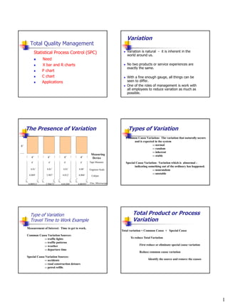
1. Variation
Total Quality Management
Statistical Process Control (SPC)  Variation is natural - it is inherent in the
world around us.
 Need
 X bar and R charts  No two products or service experiences are
exactly the same.
 P chart
 C chart  With a fine enough gauge, all things can be
 Applications seen to differ.
 One of the roles of management is work with
all employees to reduce variation as much as
possible.
The Presence of Variation Types of Variation
Common Cause Variation: The variation that naturally occurs
and is expected in the system
8’ -- normal
-- random
-- inherent
Measuring -- stable
4’ 4’ 4’ 4’ Device
4’ 4’ 4’ 4’ Tape Measure Special Cause Variation: Variation which is abnormal -
indicating something out of the ordinary has happened.
4.01’ 4.01’ 4.01’ 4.00’ Engineer Scale -- nonrandom
4.009’ 3.987’ 4.012’ 4.004’
-- unstable
Caliper
-- assignable cause variation
4.00913’ 3.98672’ 4.01204’ 4.00395’ Elec. Microscope
Type of Variation Total Product or Process
Travel Time to Work Example Variation
Measurement of Interest: Time to get to work.
Total variation = Common Cause + Special Cause
Common Cause Variation Sources:
-- traffic lights To reduce Total Variation
-- traffic patterns
-- weather First reduce or eliminate special cause variation
-- departure time
Reduce common cause variation
Special Cause Variation Sources:
-- accidents Identify the source and remove the causes
-- road construction detours
-- petrol refills
1

2. Statistical Quality Types of
Control Statistical Quality Control
 Measures performance of a process
 Uses mathematics (i.e., statistics) Statistical
Quality Control
 Involves collecting, organizing, &
interpreting data Process Acceptance
 Objective: provide statistical when Control Sampling
assignable causes of variation are
present Variables Attributes
Variables Attributes
Charts Charts
 Used to
– Control the process as products are produced
– Inspect samples of finished products
Quality Statistical Process
Characteristics Control (SPC)
Variables Attributes  Statistical technique used to ensure
 Measured values;  Has or Has not/Good process is making product to standard
e.g., weight, length, or Bad/Pass or  All process are subject to variability
volume,voltage, current etc. Fail/Accept or Reject – Natural causes: Random variations
 May be in whole or in  Characteristics for – Assignable causes: Correctable problems
fractional numbers which you focus on Machine wear, unskilled workers, poor
defects material
 Continuous random
variables  Categorical or
 Objective: Identify assignable causes
discrete random  Uses process control charts
variables
Comparing Distributions Production Output Distributions
Production Output Example What is the Difference?
Units Produced
Frequency
Plant A Plant B Plant A
99 90
100 90
100 100
90 91 92 93 94 95 96 97 98 99 100 101 102 103 104 105 106 107 108 109 110
100 110
101 110
Frequency
X
X 
500
 100 X
X 
500
 100
Plant B
n 5 n 5
No Differences!???
90 91 92 93 94 95 96 97 98 99 100 101 102 103 104 105 106 107 108 109 110
2

3. The Concept of Stability
Measure of Variation (Sigma)
99.7%
S = Standard Deviation 95%
S
(X  X ) 2
X - 3S X - 2S X - 1S
68%
X +1S X +2S X + 3S
Plant A n 1 Plant B
X (X  X ) ( X  X )2 X (X  X ) ( X  X )2
99 99-100 = -1 12 =1 90 90 -100= -10 -102 =100
100 100-100 = 0 02 = 0 90 90 -100= -10 -102 =100
100 100-100 = 0 0 2=0 100 100 -100 = 0 02 = 0
100 100-100 = 0 02 = 0 110 110 -100 = 10 102 =100
101 101-100 = 1 12 = 1 110 110 -100 = 10 102 =100
 0  2   0   400
2 400 X
S  .707 S  10
4 4 X
2 400
Plant A S  .707 Plant B S  10
4 4
X  2S  98.586 X  2S  80
X  1S  100.707 X  3S  102.121 X  1S  110 X  3S  130
X X
X  100 X  100
X  1S  99.293 X  1S  90
X  2S  101.414 X  2S  120
X  3S  97.879 X  3S  70
Under Normal Conditions: Under Normal Conditions:
68 percent of the time output will be between 99.293 and 68 percent of the time output will be between 90 and 110 units
100.707 units
95 percent of the time output will be between 80 and 120 units
95 percent of the time output will be between 98.586 and
99.7 percent of the time output will be between 70 units and
101.414 units
130 units
99.7 percent of the time output will be between 97.879 units
and 102.121 units
Control Limits Process Control Limits
Control Limits are the statistical boundaries of a process Special Cause Variation
which define the amount of variation that can be considered
as normal or inherent variation Upper Control Limit UCL=X +3
Common Cause
3 sigma control limits are most common Average
+ 3S from the mean LCL =X - 3
Lower Control Limit
If the process is in control, a value outside the control
limit will occur only 3 time in 1000 ( 1 - .997 = .003) Special Cause Variation
3

4. Relationship Between Sampling Distribution of
Population and Sampling Means, and Process
Distributions Distribution
Three population distributions Sampling
Distribution of sample means distribution of the
Beta
means
Mean of sample means  x
Normal Standard deviation of x Process
 x 
the sample means n distribution of
the sample
Uniform
 3 x  2 x 1 x xσ 1 x  2 x  3 x
(mean)
xm
95.5% of all x fall within  2  x
( mean )
99.7% of all x fall within  3 x
Theoretical Basis Theoretical Basis
of Control Charts of Control Charts
Central Limit Theorem
Central Limit Theorem Mean Standard deviation
As sample size sampling distribution
x
gets
large
becomes almost
normal regardless of X  x 
n
enough, population
distribution.
X
X 
X
X
Process Control Limit Concepts
Process Control Limit Concepts (continued)
 Control Limits Define the limits of stability  Measures inside control limits are assumed to come
 The ULC and LCL are calculated so that, if the from a stable process - Measures outside the control
process is stable, almost all of the process limits are unexpected and considered the result of a
output will be located within the control limits. special cause
 3 sigma control limits
 The most commonly used  The control limits are computed directly from the
 UCL is 3 standard deviations above the
sample data selected from the process -- The limits
average and the average are not the choice of management
or the operator - Formulas exist.
 LCL is 3 standard deviations below the
average
 If the process is stable, only about 3 out of
 The control limits define the range of inherent
1000 process outputs will fall outside the variation for the process as it currently exists, not
control limits. how we would like it to be
4

5. Control Chart Purposes Control Chart Types
Categorical or Discrete
 Show changes in data pattern Continuous Control
Numerical Data Numerical Data
– e.g., trends Charts
Make corrections before process is out of
control Variables Attributes
Charts Charts
 Show causes of changes in data
– Assignable causes
R X P C
Data outside control limits or trend in data Chart Chart Chart Chart
– Natural causes
Random variations around average
Statistical Process
Control Steps Commonly Used Control Charts
Produce Good No
Start
Provide Service  Variables data
Assign.  x-bar and R-charts
Take Sample Causes?
 x-bar and s-charts
Yes
Inspect Sample  Charts for individuals (x-charts)
Stop Process
 Attribute data
Create
Find Out Why
Control Chart  For “defectives” (p-chart, np-chart)
 For “defects” (c-chart, u-chart)
X Chart X Chart
Control Limits
UCL  x  A R From
 Type of variables control chart x 2 Table
 Shows sample means over time LCL  x  A R Sample
x 2 Range at
 Monitors process average Sample Time i
n Mean at
 Example: Weigh samples of coffee &
 xi Time i n
 Ri
compute means of samples; Plot
x  i  R  i 1
n n
# Samples
5

6. Factors for Computing
Control Chart Limits R Chart
Sample Mean Upper Lower  Type of variables control chart
Size, n Factor, A2 Range, D4 Range, D3
2 1.880 3.268 0 – Interval or ratio scaled numerical data
3 1.023 2.574 0
4 0.729 2.282 0  Shows sample ranges over time
5 0.577 2.115 0 – Difference between smallest & largest
6 0.483 2.004 0 values in inspection sample
7 0.419 1.924 0.076
8 0.373 1.864 0.136  Monitorsvariability in process
9 0.337 1.816 0.184
10 0.308 1.777 0.223  Example: Weigh samples of coffee
& compute ranges of samples; Plot
0.184
R Chart Out-of-control…when?
Control Limits
UCL R  D 4 R
From Table
LCL R  D 3R
n Sample Range at
 Ri Time i
R  i 1
n # Samples
Process is Out of Control Process is Out of Control
Trend: 8 or more points moving in the same direction - up or down
Process Control Chart
Process Control Chart
200
200
180
160
Shift in Process Average 180
140
160 Process Average Trend Up
140
UCL
Measure
120 UCL 120
Measure
100
Average 100
80 80 Average
60
LCL 60
40 40
LCL
20 20
0
0
200 201 202 203 204 205 206 207 208 209 200 201 202 203 204 205 206 207 208 209 210
Sam ple Num ber
Sample Number
6

7. Process is Out of Control Process is Out of Control
Nonrandom Patterns Present in the Data Nonrandom Patterns Present in the Data
Process Control Chart Process Control Chart
200 150
180
140
160
130
UCL
140 UCL
Measure
Measure
120
120
100
Average
110
80 100 Average
60
LCL 90
40
80
20
70
LCL
0
200 201 202 203 204 205 206 207 208 209 210 60
Sample Number 200 201 202 203 204 205 206 207 208 209 210
Sample Number
Using X and R Process Control
Signals of Control Problems Charts
 A point outside the control limits
Situation: Boise Cascade is interesting in monitoring the
 7 or more points in a row above or length of logs that arrive at a mill yard. In the long run, they
below the average (center-line) Shift want the average to be 18 feet and the variation should
continue to decline
 8 or more points in a row moving in the
same direction, up or down. Trend The process output measure is length of the logs.
 Nonrandom patterns in the data An X and R chart will be developed to monitor the
log lengths.
Use Common sense and Good Judgment
Log length Example: Data
Developing X and R Charts 30 days (subgroups) -- subgroup size
=4
 Define Process Measurement of Interest Day Log Length (feet)
 Determine Subgroup (sample) size (3-6) 1 2 3 4
 Determine data gathering methods 1 16 18 21 23
 where, how, who
2 26 20 19 19
3 20 22 18 18
 Determine number of subgroups (20-30) 4 24 16 22 20
5 17 19 24 17
 Collect Data 6 17 17 15 18
 Compute X and R for each subgroup 7 22 12 20 22
8 24 19 19 17
 Plot X and R on separate charts 9 18 18 20 14
10 17 23 19 15
 Compute Control Limits 11 20 20 17 21
 Draw Control Limits and Centerline on Charts 12 21 17 21 23
13 22 17 22 17
14 16 19 18 19
15 17 18 15 23
7

8. Log Length Data Compute X for Each
(continued) Subgroup
X
Where:
Day Log Length (feet) X = the values in
X = the subgroups
1 2 3 4
16 19 17 21 17
n = subgroup size
n
17 19 19 13 16
18 21 14 17 16
19 18 17 25 18
20 20 18 20 19
21 23 21 23 21 First Subgroup:
22 20 20 20 14
23 18 18 26 15
24 20 22 23 21
25 23 22 21 24 16 + 18 + 21 + 23
26 22 14 21 19 X1 = = 19.5
27
28
18
19
20
20
18
16
22
14 4
29 21 19 16 20
30 22 22 19 21
Compute R for Each Log Length Example: Data
Subgroup 30 days (subgroups) -- subgroup size = 4
Day Log Length (feet)
R = Subgroup High - Subgroup Low 1 2 3 4 Average = X Range = R
1 16 18 21 23 19.5 7
2 26 20 19 19 21 7
3 20 22 18 18 19.5 4
First Subgroup: 4 24 16 22 20 20.5 8
5 17 19 24 17 19.25 7
6 17 17 15 18 16.75 3
7 22 12 20 22 19 10
R1 = 23 - 16 8
9
24
18
19
18
19
20
17
14
19.75
17.5
7
6
10 17 23 19 15 18.5 8
11 20 20 17 21 19.5 4
12 21 17 21 23 20.5 6
= 7 13
14
22
16
17
19
22
18
17
19
19.5
18
5
3
15 17 18 15 23 18.25 8
Log Length Data Plot the X Values
(continued)
P lot of S ubgroup Ave ra ge s
Day Log length (feet) 50
45
1 2 3 4 Average = X Range = R
40
16 19 17 21 17 18.5 4
35
Su b g ro u p A verag e
17 19 19 13 16 16.75 6
18 21 14 17 16 17 7 30
19 18 17 25 18 19.5 8
25
20 20 18 20 19 19.25 2
21 23 21 23 21 22 2 20
22 20 20 20 14 18.5 6
15
23 18 18 26 15 19.25 11
24 20 22 23 21 21.5 3 10
25 23 22 21 24 22.5 3
5
26 22 14 21 19 19 8
27 18 20 18 22 19.5 4 0
11
13
15
17
19
21
23
25
27
29
1
3
5
7
9
28 19 20 16 14 17.25 6
29 21 19 16 20 19 5 Su b g r o u p
30 22 22 19 21 21 3
8

9. Compute Centerlines for
Plot of R Values (Ranges) Each Chart
Plot of R Values
18 X Chart:
16
14
12
X =
X i
=
577.5
= 19.25
k 30
Range (R)
10
8
6
4
R Chart:
2
R
0
171
1
3
5
7
9
11
13
15
17
19
21
23
25
27
29
i
Subgroup
R = = = 5.7
k 30
Plot the the Centerline on X Chart Plot of Centerline on R Chart
P lot of S ubgroup Ave ra ge s
Plot of R Values
50
45
18
40 16
35 14
Su b g ro u p A verag e
30 12
Range (R)
25 10
8
20
X = 19.25
6
15 R= 5.7
4
10
2
5
0
0
1
3
5
7
9
11
13
15
17
19
21
23
25
27
29
11
13
15
17
19
21
23
25
27
29
1
3
5
7
9
Su b g r o u p Subgroup
Compute the Control Limits on Compute X Control Limits
the X Chart
Table n A2 D3 D4
1 2.66
n A2 D3 D4 2 1.88 0.0 3.27
3 1.02 0.0 2.57
1 2.66 4 0.73 0.0 2.28
2 1.88 0.0 3.27 5
6
0.58
0.48
0.0
0.0
2.11
2.00
3 1.02 0.0 2.57
4 0.73 0.0 2.28 UCL = X + A 2
R = 19.25 + .73(5.7) = 23.41
5 0.58 0.0 2.11
6 0.48 0.0 2.00
LCL = X - A 2
R = 19.25 - .73(5.7) = 15.09
Now Plot the Control Limits on the X Chart
9

10. Compute Control Limits for R
Plot Control Limits on X Chart Chart
Plot of Subgroup Ave ra ge s
30
n A2 D3 D4
25 1 2.66
UCL 2 1.88 0.0 3.27
23.41
3 1.02 0.0 2.57
Subgroup Averag e
20
X = 19.25 4 0.73 0.0 2.28
5 0.58 0.0 2.11
15
15.09 6 0.48 0.0 2.00
LCL
10
5 UCL = D 4
R = 2.28(5.7) = 13.00
0
DR
11
13
15
17
19
21
23
25
27
29
1
3
5
7
9
Subgroup LCL = 3
= 0.00(5.7) = 0.00
Plot the Control Limits on R Chart
R Chart with Control Limits Utilizing the Control
Charts
Plot of R Values  Continue to Collect Subgroup data
18
 Plot Values to X and R charts
16  Examine the R Chart First - Then the X Chart
14
12
UCL 13.0  Look for Signals
 A point outside the control limits
Range (R)
10
 7 points in a row above or below the centerline
8
6
4
5.7  8 points in a row moving in the same direction
2  any nonrandom patterns
LCL
0
0.0  Take action when signal indicates
11
13
15
17
19
21
23
25
27
29
1
3
5
7
9
Subgroup
 Update Control limits when appropriate
Special control charts for variable
Special Variables Control Charts data
X bar and s-Chart
 x-bar and s charts S
(X  X ) 2
For the associated x-chart,
the control limits are derived from
n 1
 x-chart for individuals
the overall standard deviation are:
UCLS  B 4 S UCL  x  A s
x 3
From Table
LCL S  B3 S LCL  x  A s
x 3
n Sample S.D.
 Si at Time i
S  i 1
59 n # Samples
10

11. Set of observations measuring the percentage of cobalt in a chemical process
X chart for individuals
UCLx  x  3R / d
2
UCLx  x 3R / d
2
Samples of size 1, however, do not furnish enough information for process variability
measurement. Process variability can be determined by using a moving average of
ranges, or a moving range, of n successive observations. For example, a moving
range of n=2 is computed by finding the absolute difference between two successive
observations. The number of observations used in the moving range determines the
constant d2; hence, for n=2, from appendix b, d2=1.128.
UCL R  D 4 R
LCL R  D 3 R
Charts for Attributes
 Fraction nonconforming (p-chart)
 Fixed sample size
 Variable sample size
 np-chart for number nonconforming
 Charts for defects
 c-chart
 u-chart
11

12. P Charts
P Chart Example
Plywood Veneer is graded when it comes out of the
Used When the Variable of Interest is an Attribute and dryer. Sheets that graded incorrectly cause
We are Interested in Monitoring the Proportion of Items problems later in the process. Management is
in Sample that have this Attribute - interested in monitoring the rate of incorrectly
graded veneer.
Can accommodate unequal sample sizes.
Sample sizes are usually 50 or greater. The variable of interest is the proportion of
Examples:Need 20-30 samples to construct the P-chart. incorrectly graded veneer.
Each shift, n=100 sheets are selected and evaluated
Proportion of Invoices with errors
for grade. The number of mis-grades are
Proportion of Incorrectly Sorted Logs
recorded.
Proportion of Items Requiring Rework
P-Chart Data
P Charts
 Step 1:
 Collect appropriate data.
 Attribute data of the “yes/no” type
A Sheet is inspected. Is it incorrectly
graded - Yes or No?
Record the number of “Yes”
occurrences
Fraction Nonconformance
P Charts - p- Values
 Step 2:
 Calculate the fraction defective for each
subgroup.
 The fraction defective is known as the p value:
number of nonconform ances in the subgroup
p=
size of the subgroup
Key Point:
The fraction defective is always expressed as a decimal value.
Using the percentage value (i.e. 4.7% rather than .047) will
cause later computations to be inaccurate.
12

13. P Charts Plot of the p-Values
 Step 3:
 Plot the data on a graph.
 Plot each p value
P-Values and Centerline
p Charts
 Step 4:
 Compute the center line for the p chart CL = .215
and plot on the chart
 The center line of the p chart is p
total number of nonconform ances in all subgroups
p=
total number of items examined in all subgroups
429
p=  .215
2,000
p Charts P Control Chart
 Step 5
 If the sample sizes are equal, compute the 3 sigma control
limits using the following formulas - plot on control chart:
UCL = .338
Upper Control Limit
p (1 - p )
UCL = p + 3
n CL=.215
.215(1  .215)
UCL  .215  3  .338
100
Lower Control Limit LCL = .092
p (1 - p )
LCL = p - 3
n
.215(1  .215)
LCL  .215  3  .092
100
13

14. P Charts
P Charts
Step 5: Alternative - When sample sizes are
 Analyzing p Charts not equal
 p charts are analyzed using the standard tests  Compute the 3-sigma upper and lower control
for special cause variation: limits for the p chart.
 If the size of the subgroup size varies, the control limit
 A Point located outside the control limits calculations can be accomplished by two methods:
 7 or more points above or below the centerline  Compute multiple control limits based on the largest and
 8 or more points moving in the same direction smallest subgroup sizes
 Other evidence of nonrandom patterns  The two sets of control limits are plotted on the p chart. By calculating
control limits based on the largest and smallest subgroups, both the
narrowest limits (largest subgroup size) and the widest limits (smallest
subgroup size) are plotted.
 Compute separate control limits for each fraction
nonconformance.
p Charts
 Using Multiple Control Limits:
 In analyzing a control chart with multiple limits, it must be clear
that:
 Any value plotting outside the widest control limits is considered out of
control
 Any value plotting inside the narrowest control limits is considered in
control
 Only those values, if any, which plot between the two upper or two
lower control limits raise questions needing further evaluation (calculate
their individual limits)
np-Charts for number
Nonconforming
 The np-chart is a useful alternative to the
p-chart because it is often easier to
understand for production personnel-the
number of nonconforming items is more
meaningful than a fraction.
 To use the np-chart, the size of each
sample must be constant.
14

15. y1  y 2  .......  y n
np 
k
Estimate of the standard deviation
snp = np (1 - p )
wh ere p  ( n p ) / n
Upper Control Limit
UCL n p = np + 3 np (1 - p )
Lower Control Limit
LCL n p = np - 3 np (1 - p )
Chart for defects
 A defect is a single nonconforming characteristics of an
item, while a defective refers to an item that has one or
more defects.
 In some situation, quality assurance personnel mat be
interested not only in whether an item is defective but also
in how many defects it has. For example, in complex
assemblies such as electronics, the number of defects is
just as important as whether the product is defective.
 The c-chart is used to control the total number of defects
per unit when subgroup size is constant. If subgroup sizes
are variable, a u-chart is used to control the average
87 number of defects per unit.
c Charts c Charts
 Necessary Characteristics
 A c chart is a process control tool for  Subgroups must be the same size (in practical use, if
they vary less than + 15% from the average it is
charting and monitoring the number acceptable to use the average subgroup size to
compute the chart)
of attributes per unit. Each unit must  Subgroup size must be large enough to provide an
be like all other units with respect to average of at least 5 nonconformities per subgroup
size, volume, height, or other  The attribute of interest is the number of
nonconformities per unit
measurement.  Each unit may have one or more nonconformities
 The actual number of nonconformities is small
compared with the number of opportunities for
nonconformities
15

16. c Charts
C-Chart Example
 Step 1:
 Collect appropriate data.
Boise Cascade Plywood Plant has to re-patch sheets
 Attribute data of the “counting” type
when knot patches become loose or are missed during
Issue is Re-patch requirements. the initial patch line operation. The department is
Subgroup size is 3 sheets of plywood monitoring the number of re-patches.
Variable of interest is the combined number of re-patch
spots in the three sheets 3 Sheets are grouped to make sure that the average
number > 5
Re-Patch Data c Charts
 Step 2:
 Graph the data.
 The number of nonconformities is on the
vertical axis
 The sample number is on the horizontal axis
Plot The Nonconformatives
c Charts
 Step 3:
 Compute the average number and
standard deviation of defects per unit.
 Average:
total nonconformities in all samples
c =
number of samples
 Standard deviation:
s = c
16