2. 2
The Journal is a peer-reviewed publication of the R
Foundation for Statistical Computing. Communications regarding
this publication should be addressed to the editors. All articles are
copyrighted by the respective authors.
Prospective authors will find detailed and up-to-date submission
instructions on the Journal’s homepage.
Editor-in-Chief:
Peter Dalgaard
Center for Statistics
Copenhagen Business School
Solbjerg Plads 3
2000 Frederiksberg
Denmark
Editorial Board:
Vince Carey, Martyn Plummer, and Heather Turner.
Editor Programmer’s Niche:
Bill Venables
Editor Help Desk:
Uwe Ligges
Editor Book Reviews:
G. Jay Kerns
Department of Mathematics and Statistics
Youngstown State University
Youngstown, Ohio 44555-0002
USA
gkerns@ysu.edu
R Journal Homepage:
http://journal.r-project.org/
Email of editors and editorial board:
firstname.lastname@R-project.org
The R Journal Vol. 2/1, June 2010 ISSN 2073-4859
3. 3
Editorial
by Peter Dalgaard The transition from R News to The R Journal
was always about enhancing the journal’s scientific
Welcome to the 1st issue of the 2nd volume of The R credibility, with the strategic goal of allowing re-
Journal. searchers, especially young researchers, due credit
I am writing this after returning from the NORD- for their work within computational statistics. The R
STAT 2010 conference on mathematical statistics in Journal is now entering a consolidation phase, with
Voss, Norway, followed by co-teaching a course on a view to becoming a “listed journal”. To do so, we
Statistical Practice in Epidemiology in Tartu, Estonia. need to show that we have a solid scientific standing
In Voss, I had the honour of giving the opening with good editorial standards, giving submissions
lecture entitled “R: a success story with challenges”. fair treatment and being able to publish on time.
I shall spare you the challenges here, but as part of Among other things, this has taught us the concept
the talk, I described the amazing success of R, and of the “healthy backlog”: You should not publish so
a show of hands in the audience revealed that only quickly that there might be nothing to publish for the
about 10% of the audience was not familiar with R. I next issue!
also got to talk about the general role of free software We are still aiming at being a relatively fast-track
in science and I think my suggestion that closed- publication, but it may be too much to promise pub-
source software is “like a mathematician hiding his lication of even uncontentious papers within the next
proofs” was taken quite well. two issues. The fact that we now require two review-
R 2.11.1 came out recently. The 2.11.x series dis- ers on each submission is also bound to cause some
plays the usual large number of additions and cor- delay.
rections to R, but if a single major landmark is to
be pointed out, it must be the availability of a 64-bit Another obstacle to timely publication is that the
version for Windows. This has certainly been long entire work of the production of a new issue is in the
awaited, but it was held back by the lack of success hands of the editorial board, and they are generally
with a free software 64-bit toolchain (a port using four quite busy people. It is not good if a submis-
a commercial toolchain was released by REvolution sion turns out to require major copy editing of its
Computing in 2009), despite attempts since 2007. On L TEX markup and there is a new policy in place to
A
January 4th this year, however, Gong Yu sent a mes- require up-front submission of L TEX sources and fig-
A
sage to the R-devel mailing list that he had succeeded ures. For one thing, this allows reviewers to advise
in building R using a version of the MinGW-w64 on the L TEX if they can, but primarily it gives bet-
A
tools. On January 9th, Brian Ripley reported that he ter time for the editors to make sure that an accepted
was now able to build a version as well. During Win- paper is in a state where it requires minimal copy
ter and Spring this developed into almost full-blown editing before publication. We are now able to enlist
platform support in time for the release of R 2.11.0 student assistance to help with this. Longer-term, I
in April. Thanks go to Gong Yu and the “R Win- hope that it will be possible to establish a front-desk
dows Trojka”, Brian Ripley, Duncan Murdoch, and to handle submissions.
Uwe Ligges, but the groundwork by the MinGW- Finally, I would like to welcome our new Book
w64 team should also be emphasized. The MinGW- Review editor, Jay Kerns. The first book review ap-
w64 team leader, Kai Tietz, was also very helpful in pears in this issue and several more are waiting in
the porting process. the wings.
The R Journal Vol. 2/1, June 2010 ISSN 2073-4859
5. C ONTRIBUTED R ESEARCH A RTICLES 5
IsoGene: An R Package for Analyzing
Dose-response Studies in Microarray
Experiments
by Setia Pramana, Dan Lin, Philippe Haldermans, Ziv 2010), an R package called IsoGene has been devel-
Shkedy, Tobias Verbeke, Hinrich Göhlmann, An De Bondt, oped. The IsoGene package implements the testing
Willem Talloen and Luc Bijnens. procedures described by Lin et al. (2007) to identify
a subset of genes where a monotone relationship be-
Abstract IsoGene is an R package for the anal- tween gene expression and dose can be detected. In
ysis of dose-response microarray experiments to this package, the inference is based on resampling
identify gene or subsets of genes with a mono- methods, both permutations (Ge et al., 2003) and the
tone relationship between the gene expression Significance Analysis of Microarrays (SAM), Tusher
and the doses. Several testing procedures (i.e., et al., 2001. To control the False Discovery Rate (FDR)
the likelihood ratio test, Williams, Marcus, the the Benjamini Hochberg (BH) procedure (Benjamini
M, and Modified M), that take into account and Hochberg, 1995) is implemented.
the order restriction of the means with respect This paper introduces the IsoGene package with
to the increasing doses are implemented in the background information about the methodology
package. The inference is based on resampling used for analysis and its main functions. Illustrative
methods, both permutations and the Signifi- examples of analysis using this package are also pro-
cance Analysis of Microarrays (SAM). vided.
Introduction Testing for Trend in Dose Response
The exploration of dose-response relationship is im-
Microarray Experiments
portant in drug-discovery in the pharmaceutical in-
In a microarray experiment, for each gene, the fol-
dustry. The response in this type of studies can be
lowing ANOVA model is considered:
either the efficacy of a treatment or the risk associ-
ated with exposure to a treatment. Primary concerns Yij = µ(di ) + ε ij , i = 0, 1, . . . , K, j = 1, 2, . . . , ni , (1)
of such studies include establishing that a treatment
where Yij is the jth gene expression at the ith dose
has some effect and selecting a dose or doses that ap-
level, di (i = 0, 1, . . . , K) are the K+1 dose levels, µ(di )
pear efficacious and safe (Pinheiro et al., 2006). In
is the mean gene expression at each dose level, and
recent years, dose-response studies have been inte-
ε ij ∼ N (0, σ2 ). The dose levels d0 , ..., dK are strictly in-
grated with microarray technologies (Lin et al., 2010).
creasing.
Within the microarray setting, the response is gene
The null hypothesis of homogeneity of means (no
expression measured at a certain dose level. The
dose effect) is given by
aim of such a study is usually to identify a subset
of genes with expression levels that change with ex- H0 : µ(d0 ) = µ(d1 ) = · · · = µ(dK ). (2)
perimented dose levels. where µ(di ) is the mean response at dose di with
One of four main questions formulated in dose- i = 0, .., K, where i = 0 indicates the control. The al-
response studies by Ruberg (1995a, 1995b) and ternative hypotheses under the assumption of mono-
Chuang-Stein and Agresti (1997) is whether there is tone increasing and decreasing trend of means are re-
any evidence of the drug effect. To answer this ques- spectively specified by
tion, the null hypothesis of homogeneity of means
Up
(no dose effect) is tested against ordered alternatives. H1 : µ ( d0 ) ≤ µ ( d1 ) ≤ · · · ≤ µ ( d K ), (3)
Lin et al. (2007, 2010) discussed several testing pro-
cedures used in dose-response studies of microar- Down
H1 : µ ( d0 ) ≥ µ ( d1 ) ≥ · · · ≥ µ ( d K ). (4)
ray experiments. Testing procedures which take into
Down or Up
account the order restriction of means with respect For testing H0 against H1 H1 ,
estimation
to the increasing doses include Williams (Williams, of the means under both the null and alternative
1971 and 1972), Marcus (Marcus, 1976), the likeli- hypotheses is required. Under the null hypothesis,
hood ratio test (Barlow et al. 1972, and Robertson ˆ
the estimator for the mean response µ is the over-
et al. 1988), the M statistic (Hu et al., 2005) and the ˆ ˆ ˆ
all sample mean. Let µ0 , µ1 , . . . , µK be the maximum
modified M statistic (Lin et al., 2007). likelihood estimates for the means (at each dose
To carry out the analysis of dose-response mi- level) under the order restricted alternatives. Barlow
croarray experiments discussed by Lin et al. (2007, et al. (1972) and Robertson et al. (1988) showed that
The R Journal Vol. 2/1, June 2010 ISSN 2073-4859
6. 6 C ONTRIBUTED R ESEARCH A RTICLES
ˆ ˆ ˆ
µ0 , µ1 , . . . , µK are given by the isotonic regression of sum of squares under the unrestricted means. More-
the observed means. over, Hu et al. (2005) used n − K as the degrees of
In order to test H0 against H1 Down or H U p , freedom. However, the unique number of isotonic
1
Lin et al. (2007) discussed five testing procedures means is not fixed, but changes across genes. For
shown in Figure 1. The likelihood ratio test (E01 ) ¯2 that reason, Lin et al. (2007) proposed a modifica-
(Bartholomew 1961 , Barlow et al. 1972, and Robert- tion to the standard error estimator used in the M
son et al. 1988) uses the ratio between the variance statistic by replacing it with (n − I ) as the degrees of
ˆ2
under the null hypothesis (σH0 ) and the variance un- freedom, where I is the unique number of isotonic
der order restricted alternatives (σH1 ):ˆ2 means for a given gene. The five test statistics dis-
cussed above are based on the isotonic regression of
2 ˆ2
σH1 ∑ij (yij − µ j )2
ˆ the observed means. Estimation of isotonic regres-
Λ01 =
N
= . (5) sion requires the knowledge of the direction of the
ˆ2
σH0 ∑ij (yij − µ)2
ˆ trend (increasing/decreasing). In practice, the direc-
tion is not known in advance. Following Barlow et al.
Here, µ = ∑ij yij / ∑i ni is the overall mean and µi is
ˆ ˆ (1972), the IsoGene package calculates the likelihood
the isotonic mean of the ith dose level. The null hy- of the isotonic trend for both directions and chooses
2
pothesis is rejected for a "small" value of Λ01 . Hence,
N the direction for which the likelihood is maximized.
2 The Significance Analysis of Microarrays proce-
H0 is rejected for a large value of E01 = 1 − Λ01 .
¯2 N
dure (SAM, Tusher et al., 2001) can be also adapted
to the five test statistics described above. The generic
Test statistic Formula algorithm of SAM discussed by Chu et al. (2001) is
∑ij (yij −µ)2 −∑ij (yij −µi )2
ˆ ˆ implemented in this package. For the t-type test
Likelihood Ratio ¯2
E01 = ∑ij (yij −µ)2
ˆ statistics (i.e., Williams, Marcus, the M, and the M ),
Test (LRT) a fudge factor is added in the standard error of the
Williams t = (µK − y0 )/s
ˆ ¯ mean difference. For example, the SAM regularized
Marcus t = (µK − µ0 )/s
ˆ ˆ test statistic for the M is given by,
M M = ( µ K − µ0 ) / s
ˆ ˆ ˜
Modified M (M’) M = ( µ K − µ0 ) s
ˆ ˆ ˜ µ K − µ0
ˆ ˆ
M SAM = , (6)
˜
s + s0
Figure 1: Test statistics for trend test, where s =
K n where s0 is the fudge factor and is estimated from the
2 × ∑i=0 ∑ j=1 (yij − µi )2 /(ni (n − K )),
i
ˆ
n
percentiles of standard errors of all genes which min-
K
˜
s= ∑i=0 ∑ j=1 (yij − µi )2 /(n − K ),
i
ˆ imize the Coefficient of Variation (CV) of the Median
K n
s = ∑i=0 ∑ j=1 (yij − µi )2 /(n − I ), and I is the
˜ i
ˆ Absolute Deviation (MAD) of the SAM regularized
¯2
test statistics. For the F-type test statistic, such as E01 ,
unique number of isotonic means. the SAM regularized test statistic is defined by,
Williams (1971, 1972) proposed a step-down pro-
cedure to test for the dose effect. The tests are per- ˆ2 ˆ2
σH0 − σH1
¯ 2SAM =
E01 . (7)
formed sequentially from the comparison between ˆ2
σH0 + s0
the isotonic mean of the highest dose and the sam-
ple mean of the control, to the comparison between
the isotonic mean of the lowest dose and the sam- Multiplicity
ple mean of the control. The procedure stops at the
dose level where the null hypothesis (of no dose ef- In this study, a gene-by-gene analysis is carried out.
fect) is not rejected. The test statistic is shown in Fig- When many hypotheses are tested, the probability
¯
ure 1, where y0 is the sample mean at the first dose of making the type I error increases sharply with
ˆ
level (control), µi is the estimate for the mean at the the number of hypotheses tested. Hence, multiplic-
ith dose level under the ordered alternative, ni is the ity adjustments need to be performed. Dudoit et al.
number of replications at each dose level, and s2 is (2003) and Dudoit and van der Laan (2008) provided
an estimate of the variance. A few years later, Mar- extensive discussions on the multiple adjustment
cus (1976) proposed a modification to Williams’s pro- procedures in genomics. Lin et al. (2007) compared
cedure by replacing the sample mean of the control several approaches for multiplicity adjustments, and
¯
dose (y0 ) with the isotonic mean of the control dose showed the application in dose-response microarray
ˆ
(µ0 ). experiments. In the IsoGene package the inference is
Hu et al. (2005) proposed a test statistic (denoted based on resampling-based methods. The Benjamini
by M) that was similar to Marcus’ statistic, but with Hochberg (BH) procedure is used to control the FDR
the standard error estimator calculated under the or- . We use the definition of FDR from Benjamini and
dered alternatives. This is in contrast to Williams’ Hochberg (1995). The Significance Analysis of Mi-
and Marcus’ approaches that used the within group croarrays (SAM, Tusher et al., 2001) approach is also
The R Journal Vol. 2/1, June 2010 ISSN 2073-4859
7. C ONTRIBUTED R ESEARCH A RTICLES 7
considered, which estimates the FDR by using per- the testing procedures. The summary of the func-
mutations, where the FDR is computed as median tions and their descriptions are presented in Figure 2.
of the number of falsely called genes divided by the The IsoGene package can be obtained from
number of genes called significant. CRAN: http://cran.r-project.org/package=IsoGene.
The IsoGene package requires the ff and Iso pack-
ages.
Introduction to IsoGene Package
Example 1: Data Exploration
The IsoGene package provides the estimates and
p-values of five test statistics for testing for mono- To illustrate the analysis of dose-response in microar-
tone trends discussed in the previous section. The ray using IsoGene package, we use the dopamine
p-values are calculated based on a resampling proce- data. The data were obtained from a pre-clinical
dure in which the distribution of the statistic under evaluation study of an active compound (Göhlmann
the null hypothesis is approximated using permuta- and Talloen, 2009). In this study the potency of the
tions. compound was investigated. The compound had
6 dose levels (0, 0.01, 0.04, 0.16, 0.63, 2.5 mg/kg)
The main functions of the IsoGene package are
and each dose was given to four to five indepen-
IsoRawp() and IsoTestBH() which calculate the raw
dent rats. The experiment was performed using
p-values using permutations and adjust them using
Affymetrix whole-human genome chip. There are
the Benjamini-Hochberg (BH-FDR, Benjamini and
26 chips/arrays and each chip/array contains 11,562
Hochberg, 1995) and Benjamini-Yekutieli (BY-FDR,
probe sets (for simplicity, we refer to the probe sets
Benjamini and Yekutieli, 2001) procedures. The
as genes). The dopamine data set with 1000 genes is
IsoGene package also implements the Significance
provided inside the package as example data. The
Analysis of Microarrays (SAM) by using function
complete data set can be obtained on request upon
IsoTestSAM().
the first author. For this paper, the analysis is based
Function Description on the original data set (using all genes).
The example data is in an ExpressionSet object
IsoRawp() Calculates raw p-values for
each test statistic using
called dopamine. More detailed explanation of the
permutations ExpressionSet object is discussed by Falcon et al.
IsoTestBH() Adjusts raw p-values of the (2007). In order to load the object into R, the follow-
five test statistics using the ing code can be used:
BH- or BY-FDR procedure
IsoGene1() Calculates the values of the > library(affy)
five test statistics for a > library(IsoGene)
single gene > data(dopamine)
IsoGenem() Calculates the values of the > dopamine
five test statistics for all genes ExpressionSet(storageMode:lockedEnvironment)
IsoPlot() Plots the data points, sample assayData: 11562 features, 26 samples
means at each dose and element names: exprs
an isotonic regression line phenoData
(optional) sampleNames: X1, X2, ..., X26 (26 total)
IsopvaluePlot() Plots the pU p and p Down -values
varLabels and varMetadata description:
of a gene for a given test
dose: Dose Levels
IsoBHplot() Plots the raw p-values and
adjusted BH- and BY-FDR featureData
p-values featureNames: 201_at,202_at,...,11762_at
IsoGenemSAM() Calculates the values for the (11562 total)
five SAM regularized test fvarLabels and fvarMetadata
statistics description: none
IsoTestSAM() Obtains the list of significant experimentData: use 'experimentData(object)'
genes using the SAM
procedure
The IsoGene package requires the information of
Figure 2: The main IsoGene package functions. dose levels and gene expression as input. The infor-
mation of dose levels and the log2 transformed gene
The supporting functions are IsoGenem() and intensities can be extracted using the following code:
IsoGenemSAM(), which calculate the values for
> express <- data.frame(exprs(dopamine))
the five test statistics and for five SAM regular-
> dose <- pData(dopamine)$dose
ized test statistics, respectively. The functions
IsopvaluePlot(), IsoBHplot(), and IsoPlot() can For data exploration, the function IsoPlot() can
be used to display the data and show the results of be used to produce a scatterplot of the data. The
The R Journal Vol. 2/1, June 2010 ISSN 2073-4859
8. 8 C ONTRIBUTED R ESEARCH A RTICLES
function IsoPlot() has two options to specify the The output object rawpvalue is a list with four
dose levels, i.e., type ="ordinal" or "continuous". components containing the p-values for the five test
By default, the function produces the plot with statistics: two-sided p-values, one-sided p-values,
continuous dose levels and data points. To pU p -values and p Down -values. The codes to extract
add an isotonic regression line, one can specify the component containing two-sided p-values for the
add.curve=TRUE. first four genes are presented below. In a similar way,
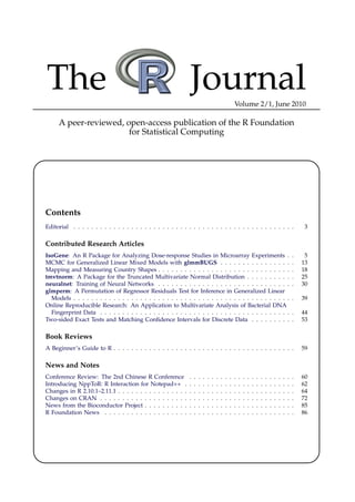
Plots of the data and an isotonic regression line one can obtain other components.
for one of the genes in the data set with dose on the > twosided.pval <- rawpvalue[[2]]
continuous and ordinal scale can be produced by us- > twosided.pval[1:4, ]
Probe.ID E2 Williams Marcus M ModM
ing the following code:
1 201_at 1.000 0.770 0.996 0.918 0.946
2 202_at 0.764 0.788 0.714 0.674 0.700
# Figure 3 3 203_at 0.154 0.094 0.122 0.120 0.134
> par(mfrow=c(1,2)) 4 204_at 0.218 0.484 0.378 0.324 0.348
> IsoPlot(dose,express[56,],type="continuous",
+ add.curve=TRUE) Once the raw p-values are obtained, one needs to
> IsoPlot(dose,express[56,],type="ordinal", adjust these p-values for multiple testing. The func-
+ add.curve=TRUE) tion IsoTestBH() is used to adjust the p-values while
controlling for the FDR. The raw p-values (e.g., rawp
), FDR level, type of multiplicity adjustment (BH-
Gene: 256_at Gene: 256_at
q q
FDR or BY-FDR) and the statistic need to be specified
q q
+
*
q
+
q
*
q
q
+
*
q
+
q
*
q
q
in following way:
q q
10
10
q q
q q
q q
+
q
* +
q
* IsoTestBH(rawp, FDR=c(0.05,0.1),
Gene Expression
Gene Expression
q q
type=c("BH","BY"), stat=c("E2",
9
9
q q
q
+
*
q
q
q
+
*
q
q
"Williams","Marcus","M","ModifM"))
8
8
q
q
q
q
IsoTestBH() produces a list of genes, which have a
q q
+
* +
* significant increasing/decreasing trend. The follow-
7
7
q q
q q
q q
+ +
ing code can be used to adjust the two-sided p-values
*
q *
q
¯2
of the E01 using the BH-FDR adjustment:
6
6
q
q q
q
q q
0.0 0.5 1.0 1.5 2.0 2.5 0 0.01 0.04 0.16 0.63 2.5
Doses Doses > E2.BH <- IsoTestBH(twosided.pval,
+ FDR = 0.05, type = "BH", stat ="E2")
> dim(E2.BH)
Figure 3: The plots produced by IsoPlot() with dose as
[1] 250 4
continuous variable (left panel) and dose as ordinal vari-
able (right panel and the real dose level is presented on The object E2.BH contains a list of significant
the x-axis). The data points are plotted as circles, while genes along with the probe ID, the corresponding
the sample means as red crosses and the fitted increasing row numbers of the gene in the original data set,
isotonic regression model as a blue solid line. the unadjusted (raw), and the BH-FDR adjusted p-
¯2
values of the E01 test statistic. In the dopamine data,
there are 250 genes tested with a significant mono-
Example 2: Resampling-based Multiple ¯2
tone trend using the likelihood ratio test (E01 ) at the
Testing 0.05 FDR level. The first four significant genes are
listed below:
In this section, we illustrate an analysis to test for
monotone trend using the five statistics presented in > E2.BH[1:4, ]
section 2 using the IsoGene package. The function Probe.ID row.num raw p-values BH adj.p-values
1 256_at 56 0 0
IsoRawp() is used to calculate raw p-values based 2 260_at 60 0 0
on permutations. The dose levels, the data frame 3 280_at 80 0 0
of the gene expression, and the number of permuta- 4 283_at 83 0 0
tions used to approximate the null distribution need
One can visualize the number of significant find-
to be specified in this function. Note that, since the
ings for the BH-FDR and BY-FDR procedures for a
permutations are generated randomly, one can use
given test statistic using the IsoBHPlot() function.
function set.seed to obtain the same random num-
ber. To calculate raw p-values for the dopamine data > # Figure 4
using 1000 permutations with seed=1234, we can use > IsoBHPlot(twosided.pval,FDR=0.05,stat="E2")
the following code:
Figure 4 shows the raw p-values (solid blue line),
> set.seed(1234) the BH-FDR adjusted p-values (dotted and dashed
> rawpvalue <- IsoRawp(dose, express, red line) and BY-FDR (dashed green line) adjusted p-
+ niter=1000) ¯2
values for the E01 .
The R Journal Vol. 2/1, June 2010 ISSN 2073-4859
9. C ONTRIBUTED R ESEARCH A RTICLES 9
2. qqstat gives the SAM regularized test statistics
E2: Adjusted p values by BH and BY obtained from permutations.
1.0
3. allfdr provides a delta table in the SAM pro-
cedure for the specified test statistic.
0.8
To extract the list of significant gene, one can do:
Adjusted P values
> SAM.ModifM.result <- SAM.ModifM[[1]]
0.6
> dim(SAM.ModifM.result)
[1] 151 6
0.4
The object SAM.ModifM.result, contains a matrix
Raw P with six columns: the Probe IDs, the correspond-
BH(FDR)
ing row numbers of the genes in the data set, the
0.2
BY(FDR)
observed SAM regularized M test statistics, the q-
values (obtained from the lowest False Discovery
0.0
Rate at which the gene is called significant), the raw
0 2000 4000 6000 8000 10000 12000 p-values obtained from the joint distribution of per-
Index mutation test statistics for all of the genes as de-
scribed by Storey and Tibshirani (2003), and the BH-
FDR adjusted p-values.
Figure 4: Plot of unadjusted, BH-FDR and BY-FDR ad-
¯2 For dopamine data, there are 151 genes found to
justed p-values for E01
have a significant monotone trend based on the SAM
regularized M test statistic with the FDR level of
Example 3: Significance Analysis of Dose- 0.05. The SAM regularized M test statistic values
response Microarray Data (SAM) along with q-values for the first four significant genes
are presented below.
The Significance Analysis of Microarrays (SAM) for
testing for the dose-response relationship under or- > SAM.ModifM.result[1:4,]
der restricted alternatives is implemented in the Iso-
Gene package as well. The function IsoTestSAM() Probe.ID row.num stat.val qvalue pvalue adj.pvalue
1 4199_at 3999 -4.142371 0.0000 3.4596e-06 0.0012903
provides a list of significant genes based on the SAM 2 4677_at 4477 -3.997728 0.0000 6.9192e-06 0.0022857
procedure. 3 7896_at 7696 -3.699228 0.0000 1.9027e-05 0.0052380
4 9287_at 9087 -3.324213 0.0108 4.4974e-05 0.0101960
> IsoTestSAM(x, y, fudge=c("none","pooled"),
+ niter=100, FDR=0.05, stat=c("E2", Note that genes are sorted increasingly based on
+ "Williams","Marcus","M","ModifM")) the SAM regularized M test statistic values (i.e.,
stat.val).
The input for this function is the dose levels
In the IsoGene package, the function
(x), gene expression (y), number of permutations
IsoSAMPlot() provides graphical outputs of the
(niter), the FDR level, the test statistic, and the
SAM procedure. This function requires the SAM
option of using fudge factor. The option fudge is
regularized test statistic values and the delta table in
used to specify the calculation the fudge factor in the
the SAM procedure, which can be obtained from the
SAM regularized test statistic. If the option fudge
resulting object of the IsoTestSAM() function, which
="pooled" is used, the fudge factor will be calculated
in this example data is called SAM.ModifM. To extract
using the method described in the SAM manual (Chu
the objects we can use the following code:
et al., 2001). If we specify fudge ="none" no fudge
factor is used. # Obtaining SAM regularized test statistic
The following code is used for analyzing the qqstat <- SAM.ModifM[[2]]
dopamine data using the SAM regularized M -test # Obtaining delta table
statistic: allfdr <- SAM.ModifM[[3]]
> set.seed(1235) We can also obtain the qqstat and allfdr from
> SAM.ModifM <- IsoTestSAM(dose, express, the functions Isoqqstat() and Isoallfdr(), respec-
+ fudge="pooled", niter=100, tively. The code for the two functions are:
+ FDR=0.05, stat="ModifM")
Isoqqstat(x, y, fudge=c("none","pooled"),niter)
The resulting object SAM.ModifM, contains three Isoallfdr(qqstat, ddelta, stat=c("E2",
components: "Williams","Marcus","M","ModifM"))
1. sign.genes1 contains a list of genes declared The examples of using the functions Isoqqstat()
significant using the SAM procedure. and Isoallfdr() are as follows:
The R Journal Vol. 2/1, June 2010 ISSN 2073-4859
10. 10 C ONTRIBUTED R ESEARCH A RTICLES
# Obtaining SAM regularized test statistic Comparison of the Results of
> qqstat <- Isoqqstat(dose, express,
+ fudge="pooled", niter=100)
Resampling-based Multiple Test-
# Obtaining delta table ing and the SAM
> allfdr <- Isoallfdr(qqstat, ,stat="ModifM")
In the previous sections we have illustrated analysis
Note that in Isoallfdr(), ddelta is left blank, with for testing a monotone trend for dose-response mi-
default values taken from the data, i.e., all the per- croarray data by using permutations and the SAM.
centiles of the standard errors of the M test statistic. The same approach can also be applied to obtain a
The two approaches above will give the same re- list of significant genes based on other statistics and
sult. Then to produces the SAM plot for the SAM other multiplicity adjustments. Figure 6 presents the
regularized M test statistic, we can use the function number of genes that are found to have a significant
IsoSAMPlot: monotone trend using five different statistics with
the FDR level of 0.05 using the two approaches.
# Figure 5 ¯2
It can be seen from Figure 6 that the E01 gives a
> IsoSAMPlot(qqstat, allfdr, FDR = 0.05, higher number of significant genes than other t-type
+ stat = "ModifM") statistics. Adding the fudge factor to the statistics
leads to a smaller number of significant genes using
the SAM procedure for the t-type test statistics as
a: plot of FDR vs. Delta b: plot of # of sign genes vs. Delta
compared to the BH-FDR procedure.
# of significant genes
10000
0.8
Number of significant genes
0.6
Test statistic BH-FDR SAM # common genes
FDR
FDR90%
6000
FDR50%
0.4
¯2
E01 250 279 200
0.2
0 2000
Williams 186 104 95
Marcus 195 117 105
0.0
0 1 2 3 4 0 1 2 3 4 M 209 158 142
delta delta M 203 151 134
c: plot of # of FP vs. Delta d: observed vs. expected statistics
Figure 6: Number of significant genes for each test
10000
q q
statistic with BH-FDR and SAM.
10
# of false positives
delta=0.72 qq
qq
q
q
qq
q
observed
q
q
q
q
q
6000
In the inference based on the permutations (BH-
5
q
q
q
q
q
qq
q
q
q
FP90% q
q
q
q
q
q
qq
qq
FP50%
qqqqq
qqqqq
qqqqq
qq
qq
qq
qq
qq
qq
qqqqqq
qqqqq
qqqqq
qq
qq
qq
qq
qq
qq
qq
qq
qq
qq
qq
qq
q
q
q
q
FDR) and the SAM, most of the genes found by the
0
q
2000
q
qq
qq
qqq
qqq
qq
qqq
qqq
qqq
qqq
qqq
qqq
qqq
qqq
qq
qq
qq
qq
qq
qqq
qq
qqq
qq
qq
qq
qq
qq
qq
qqq
qq
qq
qq
qq
qq
qqq
qq
qq
qq
qq
five statistics are in common (see Figure 6). The
qq
q
q
q q
plots of the samples and the isotonic trend of four
0
0 1 2 3 4 −2 −1 0 1 2 3
best genes that are found in all statistics and in both
delta expected
the permutations and the SAM approaches are pre-
sented in Figure 7, which have shown a significant
Figure 5: The SAM plots: a.Plot of the FDR vs. ∆; b. Plot increasing monotone trend.
of number of significant genes vs. ∆; c. Plot of number of
false positives vs. ∆; d. Plot of the observed vs. expected
test statistics.
Panel a of Figure 5 shows the FDR (either 50%
Discussion
or 90% (more stringent)) vs. ∆, from which, user
can choose the ∆ value with the corresponding de- We have shown the use of the IsoGene package for
sired FDR. The FDR 50% and FDR 90% are obtained dose-response studies within a microarray setting
from, respectively, the median and 90th percentile of along with the motivating examples. For the analy-
the number of falsely called genes (number of false sis using the SAM procedure, it should be noted that
positives) divided by the number of genes called sig- ¯2
the fudge factor in the E01 is obtained based on the
nificant, which are estimated by using permutations approach for F-type test statistic discussed by Chu
(Chu et al., 2001). Panel b shows the number of sig- et al. (2001) and should be used with caution. The
nificant genes vs. ∆, and panel c shows the number performance of such an adjustment as compared to
of false positives (either obtained from 50th or 90th the t-type test statistics has not yet been investigated
percentile) vs. ∆. Finally, panel d shows the observed in terms of power and control of the FDR. Therefore,
vs. the expected (obtained from permutations) test it is advisable to use the fudge factor in the t-type test
statistics, in which the red dots are those genes called statistics, such as the M and modified M test statis-
differentially expressed. tics.
The R Journal Vol. 2/1, June 2010 ISSN 2073-4859