1. Worcester Polytechnic Institute
100 Institute Road, Worcester, MA 01609
The views and opinions expressed herein are those of the authors and do not necessarily reflect the positions or
opinions of Worcester Polytechnic Institute. This report is a product of an education program, and is intended to
serve as partial documentation of the evaluation of academic achievement. The report should not be construed as a
working document by the reader.
PANSAT Communications:
Packet Loss and Data Throughput of a Software TNC for a Low
Earth Orbit Amateur Satellite
A Major Qualifying Project Report: submitted to the Faculty of
WORCESTER POLYTECHNIC INSTITUTE
in partial fulfillment of the requirements for the
Degree of Bachelor of Science
March 27, 2006
Project Team: Advisors:
Robert Dandekar Robert C. Labonté
bdandy02@wpi.edu rcl@wpi.edu
Zuyan Liang William R. Michalson
zuyan@wpi.edu wrm@wpi.edu
Luke Marron
lmarron@wpi.edu
Brian Martiniello
brianm22@wpi.edu

2. ii
ABSTRACT
This project was commissioned by the Electrical and Computer Engineering Department
of Worcester Polytechnic Institute to continue the design, development, and implementation of
an end-to-end command and data handling communications system for use onboard a satellite in
low earth orbit (LEO). Specifically, this project's main objectives were to evaluate alternative
software TNC solutions and calculate data throughput and bit error rate (BER) figures for data
transmissions with a satellite in LEO at the 1200 and 9600 baud rates. Recommendations for
subsequent steps to improve the calculated performance of the system are provided.

3. iii
EXECUTIVE SUMMARY
Since the 2003 – 2004 academic school year, Worcester Polytechnic Institute (WPI) has
been participating in the University Nanosat-3 (NS-3) design competition through the Powder
Metallurgy and Navigation Satellite (PANSAT) program. The program is a joint venture
between the Mechanical and Electrical & Computer Engineering departments with 3 main
objectives:
• A proof-of-concept for powder metallurgy satellite bus structures
• A test bed for global positioning system (GPS) orientation determination techniques for
spacecraft in low earth orbit (LEO)
• A measurement tool of the LEO magnetic field environment
Although the satellite design produced by WPI was not selected last year by the NS-3
board for continued development, the ECE department is continuing with the project to establish
a knowledge base that will be a valuable resource for future satellite design competitions. This
has given the department the flexibility to look back on the projects completed by the previous
project teams to evaluate, verify and/or improve upon this work.
This project had its focus within the data processing and data correction systems
requirement of the PANSAT communications system. Previous project teams had completed the
initial design, equipment procurement and setup for both the base station and satellite
communications systems. However, no quantitative data regarding the systems data
transmission capabilities have been collected. Additionally, previous teams had focused solely
on the hardware method of amateur radio communications, ignoring the emerging software
method being developing by amateur radio enthusiasts. This method utilizes inexpensive and
often readily accessible computer hardware. Space and weight savings on the spacecraft might
also be accomplished depending on the implementation method of the system. Gathering data to
characterize the performance of software amateur radio was the main objective of this project.
The two most popular packet radio transmission rates are 1200 and 9600 baud using the
AX.25 packet radio protocol. Although other transmission rates exist, satellite radio focuses
primarily on these two. To adequately assess the systems capabilities, tests were completed in
two domains: terrestrial and satellite. Terrestrial tests included both beacon and connectivity
tests. These tests produced performance figures that will allow for the prediction of data
transmission characteristics for the system. Satellite tests would then relate these performance
figures to actual satellite passes.
The state in which the ground station was found was not at the operating condition as
hoped for by previous project groups. Various system setup procedures were accomplished
before the data collection phase of the project took place. First, an accurate assessment of the
system was undertaken because confusion about the accomplishments of previous project groups
required resolution before further steps were taken. Second, simulation system configuration
took place with the procurement of equipment for establishing a second computer terminal, Uni-
Trac and Nova satellite tracking software setup and the design of a program that would record

4. iv
packet transmission statistics for analysis. After an analysis of the readily available packet radio
software, AGW Packet Engine was selected as the software TNC which was used with the UISS
terminal program for the basis of our throughput tests and calculations. Figure 0-1 shows the
final system configuration that was used to conduct the tests.
Figure 0-1: Final System Configuration
UISS allowed us to conduct both beacon and connectivity tests between our two
established computer stations. Beacon testing allowed for one station to broadcast a message up
to 80 bytes in length at set time intervals. Connectivity testing connected two stations together
and allowed them to transfer files with sizes of up to 256 kilobytes.
It is easy for one to predict the total required transmission time for a 256 kilobyte file at
both the 1200 and 9600 baud rates. It is simply the total file size in bits divided by bits per
second. This will give the total predicted number of seconds required to transmit the file. This
number then can easily be converted into minutes by dividing by 60 seconds. Figure 0-2 shows
the predicted transmission time for both 1200 and 9600 baud with a max file size of 256
kilobytes.

5. v
0 0.5 1 1.5 2 2.5
x 10
5
0
5
10
15
20
25
30
35
1200 Baud Rate
9600 Baud Rate
File Size [Bytes]
PredictedTime[minutes]
Total Time vs. File Size
Figure 0-2: 1200 and 9600 Baud Transfer Time
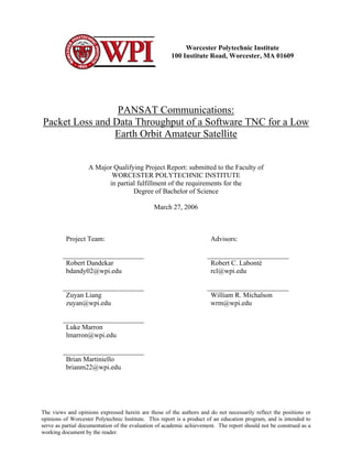
This predicted transmission time allowed us to accurately anticipate the data transmission
rates that could be observed from both baud rates. 1200 operated very close to its predicted
value. An observed packet loss rate of 0.25% was calculated through the terrestrial testing with
an average data throughput of 988.97 bits per second. This is within 85% of its advertised baud
rate. Figure 0-3 shows the predicted and actual transfer time of files varying from 0 to 256
kilobytes.
0 0.5 1 1.5 2 2.5
x 10
5
0
5
10
15
20
25
30
35
← Predicted Time (-)
File Size [Bytes]
Time[minutes]
Time vs. File Size
← Actual Time (:)
Figure 0-3: 1200 Baud, Predicted Time and Actual Time Plot
9600 baud testing produced less promising results, with an average packet loss rate of
approximately 67%. Many factors could have possibly attributed to these figures, such as poor

6. vi
software design. Because of this, connectivity tests could not be accomplished with a 9600 baud
rate.
Unfortunately, the poor performance of 9600 baud and the limited number of digital
amateur satellites orbiting the Earth prevented us from completing any satellite throughput tests.
Only 3 packet data satellites are currently in LEO orbit: GO-32, ISS, and AO-51. Of them, only
the ISS operates at 1200 baud. No contact was ever made with GO-32 and very limited receive
was found with AO-51. However, once the 9600 baud issues are resolved, throughput tests can
be conducted on AO-51. The popularity of the ISS among amateur radio enthusiasts would
make it difficult to accurately access throughput rate of 1200 baud.
Although satellite tests were not conducted, a number of tools for predicting satellite
communications performance were established. These tools focused on satellite pass modeling
and relating satellite pass parameters to a link budget calculation. The link budget determines a
signal-to-noise ratio (SNR) that can be used to assess the quality of a communications link. The
SNR for a digital communications system is referred to as the energy per bit-to-spectral noise
density ratio (Eb/No). An example of a model satellite pass can be seen in Figure 0-4. The
characteristics of this satellite pass can then be used within the link budget calculation to
determine an Eb/No value at each point of the satellite pass. An example of this calculation can
be seen in Figure 0-5.
0 100 200 300 400 500 600
200
400
600
800
1000
1200
1400
1600
1800
2000
SlantRange[km](-)
Time [sec]
Slant Range and Elevation Angle vs. Time of Sight
0 100 200 300 400 500 600
0
10
20
30
40
50
60
70
80
90
ElevationAngle[deg](:)
Figure 0-4: Example Model of a Satellite Pass

7. vii
0 100 200 300 400 500 600 700 800
0
10
20
30
40
50
60
70
Time [s]
Eb/NoRatio[dB]
Energy Per Bit (Eb) To Spectral Noise Density (No) Ratio vs. Time of Sight
Figure 0-5: Link Budget Calculation Related to Satellite Pass
The results from the link budget calculation across a satellite pass can then be compared
to established bit error rate (BER) plots to determine data transfer characteristics. This will give
some insight into the performance of the system with respect to specific satellite passes. An
example BER plot can be seen in Figure 0-6.
0 2 4 6 8 10 12 14
10
-8
10
-7
10
-6
10
-5
10
-4
10
-3
10
-2
10
-1
10
0
Eb
/N0
(dB)
BER
BPSK (Differential)
BPSK (Nondifferential)
FSK (Coherent)
FSK (Noncoherent)
Figure 0-6: Bit Error Rate Plot

8. viii
The data analysis and data prediction that was completed from this project has provided a
comprehensive summary of the current status of the PANSAT Communications satellite ground
station. Given the various challenges encountered by the team during the span of this project,
several recommendations for future communications project teams were determined. These
recommendations pertain to adjustments for the antenna, tests of a hardware-based TNC, as well
experiments with alternative software packages.
During the later stages of the project, one antenna adjustment and one reflectivity concern
were identified and should be addressed by a future PANSAT communications team. Resolving
these issues should improve the functionality of the system with several amateur satellites such
as AO-51.
The poor results of the software 9600 baud performance tests leave the actual capability
of the station’s throughput at this transmission rate a mystery. It is possible that the current
configuration of the total system is not conducive to 9600 baud transmissions or that the AGW
Packet Engine was simply not perfected for 9600 baud operation. To identify the cause of this
problem and to determine the minimum effective throughput of the system at this transmission
rate, a commercially supported hardware TNC should be acquired and fully tested.
Software TNC emulation has huge potential for both cost and weight savings on any
satellite design. The software tested during this project was freeware, which was programmed
and distributed by amateur radio hobbyists. Further exploration of freeware software TNC
programs, notably the FlexNet and Paxon software package, is encouraged. If a software TNC
solution is ultimately decided upon as the final design for the PANSAT project, it may also be
worthwhile to invest resources into an in-house developed solution.
The conclusions and subsequent recommendations from this project are the next logical
steps that should be taken to ultimately achieve a fully functioning PANSAT base
communications system, improving its overall reliability and performance. Once resolved,
future PANSAT communications teams will be able to accurately assess the transmission
capability of the ground station. This will allow for the overall software and experiment package
for the PANSAT to be configured to maximize the satellites available bandwidth.

9. ix
ACKNOWLEDGEMENTS
Our project group would like to acknowledge the following people who were integral
parts in the success of our project. We greatly appreciate the help that these people provided, and
we thank them.
• Our advisors, Professor Robert C. Labonté and Professor William R. Michalson, for their
knowledge and guidance throughout the year.
• The WPI Wireless Association, for their assistance with packet radio and testing.
• Mike Kingery of A0-51 Control Team, for his effort in trying to allow us to test our
system, and his overall insight regarding satellite communications.
• George Rossopoulos, the creator of the AGW Packet Engine software, for providing the
software and development files, and for providing responses to various issues that we
encountered.
• Mike Kastanas, for providing assistance with establishing software.
• Tyler Benoit, who dedicated his time in assisting us with developing software.

10. x
TABLE OF CONTENTS
ABSTRACT.................................................................................................................................... ii
EXECUTIVE SUMMARY ...........................................................................................................iii
ACKNOWLEDGEMENTS........................................................................................................... ix
TABLE OF CONTENTS................................................................................................................ x
AUTHORSHIP ............................................................................................................................xiii
LIST OF FIGURES ..................................................................................................................... xiv
LIST OF TABLES...................................................................................................................... xvii
1. INTRODUCTION .................................................................................................................. 1
2. PROBLEM STATEMENT..................................................................................................... 2
2.1. Problem Statement.......................................................................................................... 2
2.2. Objectives ....................................................................................................................... 2
2.2.1. Software Packet Radio Evaluation and Implementation ........................................ 2
2.2.2. Throughput and Error Rate Data Collection........................................................... 3
2.3. Project Schedule.............................................................................................................. 3
2.4. Summary......................................................................................................................... 3
3. BACKGROUND RESEARCH .............................................................................................. 4
3.1. Amateur Radio Service................................................................................................... 4
3.1.1. Amateur Radio Frequency Plan.............................................................................. 4
3.1.2. Operator Class......................................................................................................... 5
3.1.3. Amateur Radio Activities ....................................................................................... 5
3.1.4. Satellite Communications....................................................................................... 6
3.2. Amateur Satellites........................................................................................................... 7
3.2.1. The International Space Station.............................................................................. 7
3.2.2. AMSAT-OSCAR 51............................................................................................... 8
3.3. Packet Data Radio Communications .............................................................................. 8
3.3.1. AX.25...................................................................................................................... 8
3.3.2. KISS...................................................................................................................... 11
3.3.3. PACSAT ............................................................................................................... 11
3.4. Packet Radio Performance............................................................................................ 11
3.4.1. Link Budget .......................................................................................................... 12
3.4.2. Modulation and Bit Error Rate ............................................................................. 17
3.5. Equipment..................................................................................................................... 19
3.5.1. Hardware............................................................................................................... 19
3.5.2. Software................................................................................................................ 23
4. METHODOLOGY ............................................................................................................... 29
4.1. System Configuration ................................................................................................... 29
4.1.1. Equipment............................................................................................................. 29
4.1.2. Equipment Parameters .......................................................................................... 30
4.1.3. Summary............................................................................................................... 30
4.2. Test Equipment and Tools ............................................................................................ 30
4.3. Data Collection ............................................................................................................. 31
4.3.1. Terrestrial Tests .................................................................................................... 31
4.3.2. Satellite Tests........................................................................................................ 32

11. xi
4.3.3. Summary............................................................................................................... 32
4.4. Performance Prediction Tools....................................................................................... 32
4.5. Summary....................................................................................................................... 33
5. EXPERIMENTATION......................................................................................................... 34
5.1. System Configuration ................................................................................................... 34
5.1.1. Initial Configuration.............................................................................................. 34
5.1.2. Relevant Parameters.............................................................................................. 35
5.1.3. Parameter Adjustments......................................................................................... 36
5.1.4. Final Configuration............................................................................................... 39
5.1.5. Summary............................................................................................................... 44
5.2. Test Station Implementation......................................................................................... 44
5.2.1. Simulation Ground Station ................................................................................... 44
5.2.2. Packet Monitoring Program and Database ........................................................... 46
5.2.3. Summary............................................................................................................... 50
5.3. Packet Loss ................................................................................................................... 50
5.3.1. Test Statistics ........................................................................................................ 50
5.3.2. Summary............................................................................................................... 54
5.4. Throughput.................................................................................................................... 55
5.4.1. Test Statistics ........................................................................................................ 55
5.4.2. Number of Frames ................................................................................................ 58
5.4.3. Overhead............................................................................................................... 60
5.4.4. Transfer Time........................................................................................................ 61
5.4.5. Satellite Tests........................................................................................................ 65
5.4.6. Summary............................................................................................................... 65
5.5. Performance Prediction Tools....................................................................................... 66
5.5.1. Link Budget Calculation - linkbudget.m .............................................................. 66
5.5.2. Slant Range Calculation - srange.m...................................................................... 68
5.5.3. Link Budget with Slant Range - srangelink.m...................................................... 69
5.5.4. Slant Range and Elevation Calculation - srelvcalc.m........................................... 70
5.5.5. Link Budget with Slant Range and Elevation - srelvlink.m ................................. 71
5.5.6. Bit Error Rate Estimation...................................................................................... 72
5.5.7. Summary............................................................................................................... 74
6. RECOMMENDATIONS...................................................................................................... 76
6.1. Antenna Adjustments.................................................................................................... 76
6.1.1. Antenna Polarization Switching ........................................................................... 76
6.1.2. Antenna Reflectivity Concerns............................................................................. 76
6.2. Hardware TNC.......................................................................................................... 77
6.3. Software .................................................................................................................... 77
6.3.1. FlexNet and Paxon Software Package.................................................................. 77
6.3.2. In-House Developed Software TNC..................................................................... 77
6.4. Summary....................................................................................................................... 78
BIBLIOGRAPHY......................................................................................................................... 79
A. APPENDIX: Project Schedule.............................................................................................. 81
B. APPENDIX: Ground Station Equipment.............................................................................. 82
Hardware................................................................................................................................... 82
Switch Box............................................................................................................................ 82

12. xii
RIGblaster Nomic................................................................................................................. 85
Radio..................................................................................................................................... 86
Antennas ............................................................................................................................... 86
Software.................................................................................................................................... 89
Nova Installation and Setup.................................................................................................. 89
Nova Listing Utilities............................................................................................................ 94
Uni-Trac Installation and Setup............................................................................................ 97
AGW Packet Engine Installation and Setup......................................................................... 99
UISS Terminal Program Installation and Setup.................................................................. 101
Monitor Program Setup....................................................................................................... 105
FlexNet/Paxon Installation and Setup................................................................................. 107
C. APPENDIX: PANSAT Files and Folders........................................................................... 109
PANSAT Comm Programs..................................................................................................... 109
Packet Test Files and Folders ................................................................................................. 110
Project CD............................................................................................................................... 110
D. APPENDIX: UISS Reports of AO-51 Data........................................................................ 112
AO-51 Pass #3, 2/23/2006...................................................................................................... 112
AO-51 Pass #4, 2/24/2006...................................................................................................... 113
AO-51 Pass #3, 2/24/2006...................................................................................................... 114
AO-51 Pass #5, 2/26/2006...................................................................................................... 117
E. APPENDIX: MATLAB Code ............................................................................................ 119
linkbudget.m ........................................................................................................................... 119
srange.m.................................................................................................................................. 125
srangelink.m............................................................................................................................ 127
srelvcalc.m .............................................................................................................................. 131
srelvlink.m .............................................................................................................................. 132
testanalysis.m.......................................................................................................................... 136

13. xiii
AUTHORSHIP
SECTION AUTHOR
ABSTRACT Luke
EXECUTIVE SUMMARY Luke
INTRODUCTION Luke
PROBLEM STATEMENT Luke & Zuyan
BACKGROUND – Amateur Radio Service Zuyan
BACKGROUND – Amateur Satellites, Packet Radio Performance: Modulation and Bit Error Rate Luke
BACKGROUND – Packet Radio Performance: Link Budget Brian
BACKGROUND – Equipment Brian & Robert
METHODOLOGY Brian
EXPERIMENTATION – Simulation Ground Station Robert
EXPERIMENTATION – Remainder of Section Brian
RECOMMENDATIONS Robert & Luke
APPENDIX: Project Schedule Luke
APPENDIX: Ground Station Equipment – Hardware: Switch Box Luke
APPENDIX: Ground Station Equipment – Hardware: RIGblaster Nomic, Radio Brian
APPENDIX: Ground Station Equipment – Software: FlexNet/Paxon Installation and Setup Robert
APPENDIX: Ground Station Equipment – Remainder of Section Zuyan
APPENDIX: MATLAB Code Brian

14. xiv
LIST OF FIGURES
Figure 0-1: Final System Configuration ........................................................................................ iv
Figure 0-2: 1200 and 9600 Baud Transfer Time ............................................................................ v
Figure 0-3: 1200 Baud, Predicted Time and Actual Time Plot ...................................................... v
Figure 0-4: Example Model of a Satellite Pass.............................................................................. vi
Figure 0-5: Link Budget Calculation Related to Satellite Pass.....................................................vii
Figure 0-6: Bit Error Rate Plot...................................................................................................... vii
Figure 3-1: Seven Layers of OSI Reference Model........................................................................ 9
Figure 3-2: Layers 1 and 2 of OSI Model....................................................................................... 9
Figure 3-3: Information Frame Structure...................................................................................... 10
Figure 3-4: Supervisory and Unnumbered Frame Structure......................................................... 10
Figure 3-5: Figure 13-10 of Space Mission Analysis and Design, Zenith Attenuation [17] ........ 14
Figure 3-6: FSK Modulation and Frequency Spectrum Representation [17]............................... 18
Figure 3-7: BPSK Modulation and Frequency Spectrum Representation [17] ............................ 18
Figure 3-8: BER for Various Modulation Techniques [17].......................................................... 19
Figure 3-9: Example Available TNCs .......................................................................................... 20
Figure 3-10: Example Available Transceiver Radios................................................................... 21
Figure 3-11: Example Yagi Antenna............................................................................................ 22
Figure 3-12: Example Rotor and Rotor Controller....................................................................... 23
Figure 3-13: Additional Circuitry for Software TNC [20] ........................................................... 24
Figure 3-14: Examples of Terminal Programs.............................................................................. 26
Figure 3-15: Examples of Satellite Tracking Software................................................................. 28
Figure 5-1: Initial System Configuration [21] .............................................................................. 35
Figure 5-2: Final System Configuration [21]................................................................................ 39
Figure 5-3: Signal Path for Final System Configuration .............................................................. 39
Figure 5-4: UISS Terminal Program............................................................................................. 40
Figure 5-5: AGW Packet Engine Software................................................................................... 40
Figure 5-6: RIGblaster Nomic, Serial/Audio and Ethernet/Audio Connections .......................... 40
Figure 5-7: Switch Box, Front and Rear Views............................................................................ 41
Figure 5-8: ICOM IC-910 VHF/UHF All Mode Transceiver, Front and Rear Views ................. 41
Figure 5-9: MFJ HF-144/440 MHz SWR Wattmeter and Cable Connections,............................ 42
Figure 5-10: Nova for Windows Satellite Tracking Software...................................................... 43
Figure 5-11: Uni-Trac Satellite Tracking Software...................................................................... 43
Figure 5-12: Uni-Trac Hardware .................................................................................................. 43
Figure 5-13: Yaesu G-5500 Elevation-Azimuth Dual Controller, Front and Rear Views ........... 44
Figure 5-14: Simulation Station Dummy Load Schematic........................................................... 45
Figure 5-15: Simulation Station Dummy Loads........................................................................... 45
Figure 5-16: Simulation Station Data Cable................................................................................. 46
Figure 5-17: Flowchart Representation of Monitor Program ....................................................... 47
Figure 5-18: Monitor Program...................................................................................................... 48
Figure 5-19: Example Database Report........................................................................................ 49
Figure 5-20: AGWPE Delay Settings........................................................................................... 52
Figure 5-21: 1200 Baud, Number of Frames Comparison Plot.................................................... 59
Figure 5-22: 1200 Baud, Overhead Comparison Plot................................................................... 61

15. xv
Figure 5-23: 1200 Baud, Transmit Time Comparison Plot .......................................................... 62
Figure 5-24: 1200 Baud, Predicted Time and Actual Time Comparison Plot.............................. 63
Figure 5-25: 1200 Baud Predicted Time and 9600 Baud Predicted Time Comparison Plot........ 64
Figure 5-26: MATLAB Slant Range Calculation......................................................................... 68
Figure 5-27: MATLAB Eb/No Calculation.................................................................................. 70
Figure 5-28: MATLAB Slant Range and Elevation Calculation.................................................. 71
Figure 5-29: MATLAB Eb/No Calculation.................................................................................. 72
Figure 5-30: MATLAB BERTool ................................................................................................ 73
Figure 5-31: BER Plot using MATLAB BERTool....................................................................... 74
Figure A-1: Project Schedule, Term A and Term B..................................................................... 81
Figure A-2: Project Schedule, Term C and Term D..................................................................... 81
Figure B-1: ICOM IC-910H Data Socket Pins [19] ..................................................................... 83
Figure B-2: ICOM IC-910H Data Socket Connection [19].......................................................... 83
Figure B-3: Switch Box Circuitry Diagram.................................................................................. 84
Figure B-4: Switch BOX, front and Rear Views.......................................................................... 85
Figure B-5: RIGblaster Nomic Circuitry...................................................................................... 86
Figure B-6: 2 Meter (145MHz) Antenna Specifications .............................................................. 87
Figure B-7: 70 Centimeter (440MHz) Antenna Specifications.................................................... 88
Figure B-8: Nova Main Configuration Window........................................................................... 89
Figure B-9: Nova Location Input Window................................................................................... 90
Figure B-10: Nova ‘Rectangular’ View Configuration Window ................................................. 91
Figure B-11: Nova ‘View from Space’ Configuration Window .................................................. 91
Figure B-12: Nova ‘Radar’ View Configuration Window ........................................................... 92
Figure B-13: Nova ‘Setup/Antenna Rotator Configuration Window........................................... 93
Figure B-14: Nova Keplerian Elements Configuration Window ................................................. 93
Figure B-15: Nova Main Viewing Window ................................................................................. 94
Figure B-16: Nova One Observer Listing Window...................................................................... 95
Figure B-17: Nova One Observer AOS/LOS Listing Window .................................................... 95
Figure B-18: Nova Listing Setup Window................................................................................... 96
Figure B-19: Uni-Trac Main Configuration Window................................................................... 97
Figure B-20: Uni-Trac Satellite Parameter Window .................................................................... 98
Figure B-21: AGWPE Configuration List.................................................................................... 99
Figure B-22: AGWPE New Port Properties Window................................................................. 100
Figure B-23: AGWPE SoundCard Tuning Aid Window ........................................................... 100
Figure B-24: AGWPE SoundCard Volume Settings Window ................................................... 101
Figure B-25: UISS Windows Installer Error .............................................................................. 102
Figure B-26: UISS Call Sign Window........................................................................................ 102
Figure B-27: UISS Main Viewing Window ............................................................................... 102
Figure B-28: UISS Connection Window.................................................................................... 103
Figure B-29: UISS Beacon Configuration Window................................................................... 104
Figure B-30: UISS Main Viewing Window, Beacon On ........................................................... 104
Figure B-31: Monitor Program Main Viewing Window............................................................ 105
Figure B-32: Monitor Program Test Window ............................................................................ 106
Figure B-33: Monitor Program Test Files Window.................................................................... 106
Figure B-34: FlexNet Operating Window .................................................................................. 107
Figure B-35: FlexNet SoundModem Configuration Window .................................................... 107

16. xvi
Figure B-36: Paxon Terminal Window....................................................................................... 108
Figure C-1: ‘PANSAT Comm Programs’ Folder Contents........................................................ 109
Figure C-2: ‘Packet Test Files and Folders’ Contents................................................................ 110

17. xvii
LIST OF TABLES
Table 3-1: FCC Authorized Amateur Radio Frequency Bands and Segments [5]......................... 4
Table 3-2: Privileges for Different Operator Classes [5]................................................................ 5
Table 3-3: FCC Authorized Amateur Radio Satellite Frequency Bands and Segments [9]........... 7
Table 3-4: Link Budget Input Parameters for Transmitter ........................................................... 13
Table 3-5: Link Budget Input Parameters for Path Loss .............................................................. 14
Table 3-6: Link Budget Input Parameters for Receiver................................................................ 15
Table 3-7: Link Budget Input Parameters for Eb/No.................................................................... 16
Table 3-8: Table 13-10 of Space Mission Analysis and Design, System Noise Temperature [17] ......... 16
Table 3-9: TNC Comparison and Analysis................................................................................... 21
Table 3-10: Deciphering Frame Headers [20] .............................................................................. 27
Table 5-1: Packet Loss from 1200 Baud Beacon Tests................................................................ 51
Table 5-2: Packet Loss from 9600 Baud Beacon Tests................................................................ 51
Table 5-3: Packet Loss from 9600 Baud Manual Tests with Delay Adjustments........................ 53
Table 5-4: Packet Loss from 1200 Baud Connection Tests 1....................................................... 53
Table 5-5: Packet Loss from 1200 Baud Connection Tests 2....................................................... 54
Table 5-6: Example 1200 Baud Connection Test Analysis.......................................................... 57
Table 5-7: Averages from 1200 Baud Connection Test Analysis ................................................ 58
Table 5-8: Throughput Rate Calculations..................................................................................... 65
Table 5-9: Example Link Budget Calculation .............................................................................. 67
Table B-1: MAIN Band Pin Colors and Descriptions .................................................................. 84
Table B-2: SUB Band Pin Colors and Descriptions..................................................................... 84
Table B-3:: RJ45 Connector Pin Colors and Descriptions ........................................................... 84
Table C-1: Project CD Folder Descriptions................................................................................ 111

18. 1
1. INTRODUCTION
Since the 2003 – 2004 academic school year, the Worcester Polytechnic Institute has
been participating in the University Nanosat-3 (NS-3) design competition sponsored by the
American Institute of Aeronautics and Astronautics (AIAA), the National Aeronautics and Space
Administration Goddard Space Flight Center (NASA GSFC), the Air Force Office of Scientific
Research (AFOSR) and the Air Force Research Laboratory Space Vehicles Directorate
(AFRL/VS). The project’s objectives are “to educate and train the future workforce through a
national student satellite design and fabrication competition and to enable small satellite research
and development, payload development, integration and flight test [1].” From this, WPI founded
the Powder Metallurgy and Navigation Satellite (PANSAT) program, a joint venture between the
Mechanical and Electrical and Computer Engineering departments.
The WPI PANSAT project established 3 objectives specific objectives that the program
would accomplish [2]:
• A proof-of-concept for powder metallurgy satellite bus structures
• A test bed for global positioning system (GPS) orientation determination techniques for
spacecraft in low earth orbit (LEO)
• A measurement tool of the LEO magnetic field environment
Although WPI’s satellite design was not selected last year by the NS-3 board for
continued development, the ECE department is continuing with the project to establish a
knowledge base that will be a valuable resource for future satellite design competitions. This has
given the department the flexibility to look back on the projects completed by the previous
project teams to evaluate, verify and / or improve upon their work.
1.1. Report Summary
This project report is divided into six chapters. Chapter Two will present the problem
statement and the two main objectives that the project was separated into. Chapter Three will
present background information on:
• The Amateur Radio Service
• Amateur Satellites
• Packet Data Radio Communications
• Equipment, both Software and Hardware
• Performance Prediction Methods
Chapter Four will cover the project methodology, including:
• System Configuration
• Experiment Design
• Performance Prediction Tools
Chapter Five will present the results and analysis of all completed tests, including:
• Error Rates
• Data Throughput Rates
• Performance Prediction Tools
Finally, Chapter Six will present recommendations for future PANSAT projects.

19. 2
2. PROBLEM STATEMENT
This chapter presents our group’s established problem statement, objectives, and project
schedule.
2.1. Problem Statement
The defined problem statement for all PANSAT communications projects is to:
Design, develop, build, and test an end to end ultra high frequency (UHF) communications
system for command and data handling (CDH) between Worcester Polytechnic Institute (WPI)
and a low earth orbit (LEO) nanosatellite as well as implement tracking software, data
processing and data correction systems.[2]
This project was focused within the data processing and data correction systems
requirement of the PANSAT communications system. Previous project teams have completed
the initial design, equipment procurement and setup for both the base station and satellite
communications systems. However, no quantitative data regarding the systems data
transmission capabilities has been collected. Additionally, previous teams have been focused
solely on the hardware method of amateur radio communications, ignoring the emerging
software method being developing by amateur radio enthusiasts. This project specifically
focused on evaluating the software method of amateur packet radio communications and the
collection of throughput and error rate data for connections with amateur LEO satellites.
2.2. Objectives
Two project objectives were derived from the problem statement: evaluating software
packet radio implementation methods and collecting throughput and error rate data for amateur
packet radio.
2.2.1. Software Packet Radio Evaluation and Implementation
The technological advances in personal computing within the last 10 years have given
personal computers adequate processing power to perform the functions of amateur radio
terminal node controllers in a software environment. This method utilizes inexpensive and often
readily accessible computer hardware. Space and weight savings on the spacecraft might also be
accomplished depending on the implementation method of the system. Research will be
conducted to explore current software packet radio practices and to determine whether this
method of packet radio is worth developing as an alternative for the PANSAT’s communications
system.

20. 3
2.2.2. Throughput and Error Rate Data Collection
The ultimate goal of this project is to quantify the packet radio throughput rates of a low
earth orbit satellite. Amateur radio currently operates at both 1200 and 9600 baud for packet
communications. Throughput testing will produce data that will allow us to establish expected
data transfer rates and packet error rates for a low earth orbit amateur satellite. This knowledge
will then be used by future PANSAT teams to establish data loads for the satellite and allow the
software and onboard experiments to be adjusted to maximize the satellites available bandwidth.
2.3. Project Schedule
This project was completed over the course of the 2005-2006 academic school year.
Term A’05 was used to familiarize the team with amateur radio, including all team members
acquiring a technician class amateur radio license from the FCC. Term B’05 was used for
research and experiment preparation, with Term C’06 being the experimentation and data
collection period. Term D’06 was used for data analysis and report writing. See APPENDIX:
Project Schedule for the detailed project schedule.
2.4. Summary
The goal of all PANSAT Communications teams is to design, develop, build, and test an
end to end data communications system for a satellite in a low earth orbit. The PANSAT
communications team will focus on evaluating software packet radio methods and also collecting
data throughput rates. The findings of this project will then be used to formulate next steps and
provide guidance for future PANSAT communications teams.

21. 4
3. BACKGROUND RESEARCH
Background research provides the basic knowledge that is required to adequately assess
and accomplish the project’s defined objectives. This section will provide information that is
necessary to operate amateur packet radio at the PANSAT base communications system for any
new to amateur packet radio user.
3.1. Amateur Radio Service
Amateur Radio Service presents “an opportunity for self-training, intercommunication,
and technical investigations [3].” This service is shared by “authorized persons [who] interested
in radio technique solely with a personal aim and without pecuniary interest [4].” In order to
operate an amateur station, a person must possess an amateur radio license issued from the
Federal Communications Commission (FCC). Voice, digital data, and Morse code transmissions
are the three most common methods amateur radio as performed around the world. Under proper
operating conditions, amateur radio enthusiasts have the ability to communicate around the
globe.
3.1.1. Amateur Radio Frequency Plan
In the United States, the FCC regulates the radio wave spectrum and designates the
frequency subdivisions in which radio communication may be performed. The FCC has
authorized the frequency bands shown in Table 3-1 for the Amateur Radio Service.
Authorized Band Authorized Segments
160m 1.8 – 2.0 MHz
80m 3.50 – 4.0 MHz
60m 5.3305 – 5.4035 MHz
40m 7.0 – 7.30 MHz
30m 10.10 – 10.15 MHz
20m 14.0 – 14.350 MHz
17m 18.068 – 18.168 MHz
15m 21.0 – 21.450 MHz
12m 24.890 – 24.990 MHz
10m 28.0 – 29.70 MHz
6m 50.0 – 54.0 MHz
2m 144.0 – 148.0 MHz
1.25m 222.0 – 225.0 MHz
70cm 420.0 – 450.0 MHz
33cm 902.0 – 928.0 MHz
23cm 1.240 – 1.30 GHz
Higher Frequencies Above 2.30 GHz
Table 3-1: FCC Authorized Amateur Radio Frequency Bands and Segments [5]

22. 5
3.1.2. Operator Class
The FCC is responsible for licensing all amateur radio operators as Technician, General,
Amateur Extra, Novice, Technician Plus, or Advanced class operators depending on their
“degree of skill and knowledge in operating a station [6].” Each class is authorized with varying
levels of privileges to operate the different bands. Table 3-2 shows the difference privileges for
different types of class holder:
Operator Classes Frequency Bands
Technician 6m, 2m, 1.25m, 70cm, 33cm, 23cm, Higher Frequencies
General 160m, 80m, 40m, 30m, 20m, 17m, 15m, 12m, 10m, 6m, 2m, 1.25m, 70cm,
33cm, 23cm, Higher Frequencies
Amateur Extra 160m, 80m, 40m, 30m, 20m, 17m, 15m, 12m, 10m, 6m, 2m, 1.25m, 70cm,
33cm, 23cm, Higher Frequencies
Novice 80m, 40m, 15m, 10m, 1.25m, 23cm
Technician Plan 80m, 40m, 15m, 10m, 6m, 2m, 1.25m, 70cn, 33cm, 23cm, Higher
Frequencies
Advanced 160m, 80m, 40m, 30m, 20m, 17m, 15m, 12m, 10m, 6m, 2m, 1.25m, 70cm,
33cm, 23cm, Higher Frequencies
Table 3-2: Privileges for Different Operator Classes [5]
3.1.3. Amateur Radio Activities
“Amateur Radio Service is well known for its flexibility in satisfying the wants and
needs of hams [amateurs]. This can be accomplished individually or with two-way
communications with others. It can be used for relaxation, excitement, or as a way to stretch
one’s mental and physical horizons.” Some of the activities practiced by amateur radio
enthusiasts are shown below [2]:
Nets: This refers to traffic nets, where amateurs transfer messages on behalf of other
hams or non-hams, and casual nets, where groups of hams with common interest meet to
share information and discuss pertinent anecdotes.
Rag-chewing: The simple act of conversing with old and new friends using amateur
radio communications.
Amateur Radio Education: Amateur radio operators spend a great deal of time
educating their peers and new amateurs.
Emergency Communication: During emergencies and disasters, hams may have the
only reliable means of communicating with the outside world.
Direction Finding: Amateurs organize fox hunts where a beacon transmitter is hidden
and a competition is held to find the hidden transmitter.

23. 6
Satellite Operation: Using amateur satellites, hams are able to contact each other even
across the globe.
Repeaters: A repeater is an amateur station that receives transmissions from mobile or
fixed amateur stations and rebroadcasts the transmissions over a wide area to facilitate
communications between amateurs with low power radios.
Image Communications: A means to transferring images between amateur radio
operators.
Digital Communications: Using a computer to communicate with local and distant
stations.
EME (Earth-Moon-Earth), Meteor Scatter and Aurora: Making contacts by bouncing
signals off the moon and the trails of meteors and auroras.
3.1.4. Satellite Communications
“Satellite communications is the transfer of information among a constellation of
satellites and ground station[s] [2].” Basically, it is an artificial satellite that receives radio,
television, and other signals in space and reflects or rebroadcasts them back to earth. When it
was first introduced in the early 1960s, it changed the way people thought about communications
and information exchange. Satellites, defined “as manufactured object[s] or vehicle[s] intended
to orbit the earth, the moon, or another celestial body [7],” are located in orbit at an elevation of
at least 150 miles. Associated with a satellites orbit is its effective footprint, or the area it is able
to broadcast its signal over at any given time. The size of the footprint is directly related to the
altitude of the satellite’s orbit; the higher the orbit, the larger the footprint. With this
characteristic, satellites can cover areas larger than those serviced by most terrestrial antennas,
including isolated areas where there is no established telecommunications infrastructure. Early
applications for satellite communications were designed for long distance telephone calls.
Today, voice communications remains one of the most important applications for satellite
communication.
Depending on the altitude of a satellites orbit, they can be classified as either
Geostationary Orbit Satellites (GEOSAT) or Low Earth Orbit satellites (LEOSAT). “GEOSATs
circle the earth in geostationary orbit, an orbit that matches the rate of rotation of the earth.”
GEOSATs are usually launched at an orbit that is 22,300 miles or 35,900 kilometers above the
ground. With that altitude, a satellite can communicate with about one-third of the ground
station at all times. In contract to GEOSATs, LEOSATs are launched at a lower orbit and rotate
the earth at a much higher speed. It is only 200 to 500 miles or 320 to 800 kilometers above the
ground and orbits the earth every two to three hours [8].
All amateur radio satellites are LEOSATs. In addition to the authorized amateur radio
bands from Table 3-1, the FCC has also allocated addition frequency bands for amateur radio
satellite communication which can be seen in Table 3-3.

24. 7
Authorized Bands Authorized Segments
40m 7.0-7.1MHz
20m 14.0 – 14.25 MHz
17m 18.068 – 18.168MHz
15m 21.0 – 21.45MHz
12m 24.89 – 24.99MHz
10m 28.0 – 29.7MHz
2m 144.0 – 146MHz
5mm 5.83 – 5.85GHz
2mm 10.45 – 10.50GHz
1mm 24.0 – 24.05GHz
0.6mm 47.0 – 47.2GHz
0.4mm 75.5 – 76.0GHz
0.3mm 77.0 – 81.0GHz
0.2mm 142.0 – 149.0GHz
0.1mm 241.0 – 250.0GHz
Table 3-3: FCC Authorized Amateur Radio Satellite Frequency Bands and Segments [9]
3.2. Amateur Satellites
As of February of 2006, there are nineteen amateur radio satellites that are in a LEO
surrounding planet earth. Of these, three are digital satellites and have the capability to handle
packet radio communications: the International Space Station (ISS or Zarya), AMSAT-OSCAR
51 (Echo or AO-51), and Gurwin TechSat1b (GO-32) [10]. The ISS and Echo were the focus of
our connection efforts because of their established support community and 100% operational
status. The status of current satellites can be found at http://www.amsat.org.
3.2.1. The International Space Station
Amateur Radio on the International Space Station (ARISS) is a joint venture between the
Russian Space Agency and the National Aeronautics and Space Administration (NASA) on the
International Space Station. Although the station is still being constructed, amateur radio is
active on the station. All astronauts living in the station have amateur radio licenses and
frequently make contacts to amateur radio operators around the world. In the digital
communications realm, the ISS acts as a digipeater for terrestrial APRS traffic, including its own
position [11]. Automatic Position Reporting System, APRS, is a tactical radio amateur network
that utilizes GPS coordinates to keep real time positioning of participating amateur radio
operators around the world.

25. 8
3.2.2. AMSAT-OSCAR 51
AMSAT-OSCAR 51, AO-51 or Echo, is the newest AMSAT currently in orbit. It was
funded by the AMSAT USA corporation and was launched out of the Russian Cosmodrome in
December of 2004. Echo operates in the analog, digital (9600 baud uplink / downlink, 36000
baud downlink) and PSK-31 modes. However, the satellite rarely operates in all three modes at
one given time. Check http://www.amsat.org/amsat-new/echo/ControlTeam.php for the monthly
operational schedule of the satellite [12].
3.3. Packet Data Radio Communications
Packet data radio communications developed out of the desire to create a wireless
medium for data transfer, based on the packet data communications that already existed in
projects such as ARPANET in the mid-1960s. The first packet radio network was established by
the University of Hawaii and was fittingly called the ALOHANET in 1969. The first amateur
packet radio communications were made on May 31, 1979 in Montreal, Canada.
Packet radio has some inherent advantages over amateur radio data communications;
built in error correction, automated control and the flexibility to be adapted to a wide range of
system/communications requirements. This flexibility has allowed it to be adapted for data
exchange, real-time communications, APRS and satellite communications [13].
3.3.1. AX.25
AX.25 is the primary protocol that is used for packet radio communications. An
extension of the X.25 wired data transfer protocol, it associates packet formation and
transmission into a standard that is used for packet data radio communications. The AX.25
protocol defines a standard of packet transmission to monitor and control packet traffic so that
packets are delivered reliably. The development of this protocol has led to other sub-protocols
that provide additional communication features for amateur satellite operators and licensed
technicians [13].
AX.25 comprises layer 1, 2 and 7 of the Open Systems Interconnect (OSI) model, as
defined by the International Standards Organization (ISO), for interconnecting different
computer systems, which can be seen in Figure 3-1.

26. 9
Figure 3-1: Seven Layers of OSI Reference Model
Layer 1 and layer 2, the Physical and Data Link Layers respectively, are the final two
layers where the AX.25 protocol is defined and implemented. Figure 3-2 shows the relationship
between the two layers and how a packet progresses from binary bits into a transmittable audio
packet that can be distinguished by another amateur radio user. SAP stands for Service Access
Point [14].
Figure 3-2: Layers 1 and 2 of OSI Model

27. 10
As with all link layer packet radio transmissions, AX.25 packets, also called frames, are
divided into small blocks of data called fields. These fields contain header information that
identifies the destination of the frame, its contents, and its sequence among the total frames.
This allows the receiving party to reconstruct the transmitted data. There are three basic frames
used for AX.25 applications: Information Frame (I Frame), Supervisory Frame (S Frame), and
Unnumbered Frame (U Frame). The structure of these frames can be seen in Figure 3-3 and
Figure 3-4.
Figure 3-3: Information Frame Structure
Figure 3-4: Supervisory and Unnumbered Frame Structure
The only difference between the three frame types, as you can see in the figures above, is that
Information frames contain Protocol Identifier (PID) field. This will be described in further
detail in below.
Flag Field: The Flag Field, which is one octet long, is used to identify both the beginning
and end of the current frame. 01111110 (7E hex) is used to distinguish a flag.
Address Field: This field contains both the addresses of the receiving and sending
parties.
Control Field: The control field identifies the type of frame being passed and also
controls some parameters within the Data Link Layer (Layer 2) of the AX.25 protocol.
Protocol Identifier (PID) Field: This field, as noted above, is only present in
Information Frames. It is used to identify if any Layer 3 protocols are being used.
Information Field: This field contains the data that is being sent between the two
parties. It is only utilized in Information Frames and zero padded in others to adequately
separate it from the Flag Check Field.
Frame-Check Sequence: Both the sender and the receiver calculate a sixteen-bit number
to check against each other, ensuring that the data did not become corrupt during the data
transmission.
This breakdown of the AX.25 protocol is all that is required to successfully implement
the protocol and understand its functionality. If a more detailed description of the protocol is
desired, please refer to AX.25 Link Access Protocol for Amateur Packet Radio, V2.2 paper
published by the Tuscon amateur Packet Radio Corporation [14].

28. 11
3.3.2. KISS
The KISS protocol acts as the data transmission protocol between the PC and a hardware-
based TNC through a RS232 serial port. It has defined commands that both automate certain
TNC functions and allow the user to adjust the parameters of the TNC through a terminal
window or other interface program. It is not an amateur radio transmission protocol [15].
3.3.3. PACSAT
The PACSAT protocol is a sub-protocol within AX.25. It was developed by Harold
Price, callsign NK6N, and Jeff Ward, callsign G0/K8KA, at the University of Surrey, United
Kingdom in the early 1990s. Specifically, they set out to “make the best use of a bandwidth-
limited low earth orbiting digital store-and-forward system with a worldwide, unstructured,
heterogeneous user base [16]” and eventually established the packet communications
architecture for AMSATs that is in use today. The PACSAT protocol adds additional header
information to each AX.25 data packet, which helps identify the data contents of the packet for
all users. This keeps a satellite from having to acknowledge and resend identical data to multiple
users one at a time. The header information also contains enough data that the receiving party is
able to determine if they have any missing portions of received data and can then request a
resend of that data only.
This concept led to the establishment of parameters for file serving, store and forward
capabilities and bulletin board systems (BBS) for LEO satellites. However, the advent of the
Internet and other data communications technologies has mostly rendered these services
obsolete.
3.4. Packet Radio Performance
The performance of packet radio and digital communications in general is reliant on
many factors. These factors include path loss characteristics through environmental propagation
and system equipment capabilities at maintaining signal integrity. However, a simplified
analysis of a digital communications system can be performed by calculating a link budget for
the system. A link budget is a summation of the power and gain capabilities of all the factors
that affect a signal along its propagation. By performing a link budget calculation, one is able to
gain insight into these factors in a manner that is not too complex. The result of a link budget
calculation is a signal-to-noise ratio (SNR) that provides a measure of the relative strength of the
signal as compared to ambient noise due to equipment and the environment.
A link budget calculation is also important to digital communications because it can be
used to indicate a bit error rate (BER) which is a primary concern for data transfer. Much
research has been performed that has related SNR values to BER values with respect to digital
data rates and modulation techniques. Therefore, by performing a link budget calculation and
analyzing the data rate and modulation techniques used for a digital communications system, a
theoretical BER can be determined that will predict the performance of that system.

29. 12
3.4.1. Link Budget
As previously mentioned, a link budget is a summation of the power and gain capabilities
of a digital communications system. The link budget can be performed using a summation
through the use of decibels (dB) which are logarithmic ratio values found by the following
equation:
)(log10 10 XX dB =
where X is the units value to be converted to decibels; for example, power and gain.
With respect to a satellite communications system, the link budget analyzes the power
output of the ground station and the gain provided by the antennas, the losses that occur through
environmental propagation, and the gain provided by the receiving station and its antennas.
Various parameters also play a role within these signal paths and will be described further. For a
satellite communications system, it is easiest to describe the link budget in three main parts: the
transmitter, path loss, and receiver. There are various ways to calculate a link budget for a
communications system. The method described here was determined from Space Mission
Analysis and Design by James R. Wertz and Wiley J. Larson (editors) [17].
This method determines an energy per bit (Eb) to the spectral noise density (No), Eb/No,
value. The Eb/No ratio is a signal to noise ratio for a digital communications system. This value
can be viewed as the power allocated for each bit of data that is transmitted. This method was
used because of the robustness it provided in describing the system completely. Some
parameters and steps have been manipulated slightly to better conform to the characteristics of
the PANSAT ground station. Derivations for the presented equations were not included in all
cases, but taking a moment to consider them will allow you to gain an idea of their origin.
There are a number of input parameters that need to be established to begin the analysis
of the transmitter. These parameters can be seen in Table 3-4. P is the output power of the
transmitter, or transceiver radio, and lL is an estimation of the losses that may occur along the
transmission line from the transceiver to the radio. ptG and tθ are the gain of the transmit
antenna and the antenna beamwidth, respectively. These are characteristics of the antenna that
can be found in the antenna specifications. For dish antennas whose antenna patterns are not
simply directional, these values can also be determined through equations found in Space
Mission Analysis and Design. vθ is the minimum view elevation angle, and is an estimation of
the angle at which the satellite is first seen. This is necessary to consider because the terrain
surrounding a ground station may not allow a satellite to be seen as soon as it has passed above
the horizon. R and Altitude are simply the radius of the earth and the altitude of the satellite,
respectively.

30. 13
P Transmitter output power, expressed in watts (W).
lL Transmitter line loss, expressed in decibels (dB).
ptG Transmit antenna gain, expressed in decibels (dB).
tθ Transmit antenna beamwidth, expressed in degrees (°).
vθ Minimum view elevation angle, expressed in degrees (°).
R Radius of the earth, expressed in kilometers (km).
Altitude Altitude of the satellite, expressed in kilometers (km).
Table 3-4: Link Budget Input Parameters for Transmitter
The first step for calculations involving the transmitter is to convert the output power to a
decibel value using Equation 1 resulting in a dBW value.
Transmitter Power )(log10 10 PPdB = [Equation 1]
Next, the gain of the antenna is calculated after assuming loss due to the pointing offset
between the transmit and receive antennas. This pointing offset is the angle difference from
beam center from transmitter to receiver, a maximum of which occurs when the satellite is first
seen. This angle is found through Equation 2, which uses the Law of Sines based on a triangle
with the center of the earth, the ground station, and the satellite as vertices.
Transmit Antenna Pointing Offset )
)90sin(
(sin 1
AltitudeR
R
e v
t
+
+°
= − θ
[Equation 2]
The loss due to this pointing offset can be found using Equation 3.
Transmit Antenna Pointing Loss
2
)(12
t
te
L
θ
θ −= [Equation 3]
The net transmit antenna gain can then be found by Equation 4. This simply adds the loss
due to antenna pointing to the gain of the transmit antennas.
Net Transmit Antenna Gain θLGG ptt += [Equation 4]
Finally, the equivalent isotropic radiated power (EIRP) is found using Equation 5. EIRP
is defined as “the amount of power that would have to be emitted by an isotropic antenna,
[which] evenly distributes power in all directions, to produce the peak power density observed in
the direction of maximum antenna gain [18].” In this case, the EIRP can simply be viewed as the
maximum radiated power. It is found by adding the line loss and net antenna gain to the output
power of the transmitter.
Equivalent Isotropic Radiated Power tldB GLPEIRP ++= [Equation 5]

31. 14
The radiated power is then subject to space and atmospheric attenuation factors along the
path of propagation. To analyze these factors, some input parameters need to be established as
well. These parameters can be seen in Table 3-5. R and Altitude are simply the radius of the
earth and the altitude of the satellite, respectively. f is the frequency of the carrier signal and c
is the speed of light. re is the pointing offset of the receiver. This is similar to the
corresponding transmitter parameter, but is a constant for the receiver to take into account an
inherent pointing difference. vθ is again the minimum view elevation angle, and aZ is the
theoretical zenith attenuation. This value is an estimate of the loss that occurs when a signal
propagates through the atmosphere at a 90° elevation. This value can be determined based on
the carrier frequency and the height above sea level of the ground station using Figure 13-10 of
[17], which is replicated here in Figure 3-5.
R Radius of the earth, expressed in kilometers (km).
Altitude Altitude of the satellite, expressed in kilometers (km).
f Frequency of the carrier signal, expressed in gigahertz (GHz), megahertz (MHz), or Hertz (Hz).
c Speed of light, 3e8, expressed in meters per second (m/s).
re Receive antenna pointing offset, expressed in degrees (°).
vθ Minimum view elevation angle, expressed in degrees (°).
aZ Theoretical one way zenith attenuation, expressed in decibels (dB).
Table 3-5: Link Budget Input Parameters for Path Loss
Figure 3-5: Figure 13-10 of Space Mission Analysis and Design, Zenith Attenuation [17]
The slant range from ground station to satellite must be found to determine the distance
the signal must propagate. This can be done by using Equation 6, which uses the Law of Sines
to determine the slant range at the minimum view elevation angle. This was done because the
longest slant range, which will yield the most attenuation, occurs when the satellite is first seen.

32. 15
Slant Range )
)90sin(
))90(180sin(
)((
v
vre
AltitudeRS
θ
θ
+
+−−
+= [Equation 6]
The slant range is then used to determine the space loss through Equation 7. The space
loss, the attenuation through free space, is a function of wavelength which can be determined
from the carrier frequency and the velocity of the signal, which is the speed of light. This
explains the use of f and c in the following equation.
Space Loss )(log20)(log20)4(log20)(log20 10101010 Hzs fScL −−−= π [Equation 7]
Losses also occur due to atmospheric conditions, as mentioned by the zenith attenuation
parameter above. The minimum loss occurs when the signal propagates through the atmosphere
at zenith. Therefore, the zenith attenuation parameter is the minimum loss that occurs due to the
atmosphere. The loss at smaller angle values can be found by simply scaling the zenith
attenuation by )sin( vθ . The loss due to the atmosphere can then be found by using Equation 8.
Propagation and Polarization
Path Loss )sin( v
a
a
Z
L
θ
= [Equation 8]
There are also a number if input parameters needed to analyze the receiver. These
parameters can be seen in Table 3-6. rD is the diameter of the antenna, and is used in predicting
the antenna gain of a satellite which may not use a directional antenna system. η is the
efficiency of the antenna, and is also an estimated value. It is a function of imperfections in the
antenna such as deviations of the reflector surface and feed losses. Values of 0.6 to 0.7 typically
occur in high quality ground antennas [17]. The remaining parameters have been previously
described.
rD Receive antenna diameter, expressed in meters (m).
η Receive antenna efficiency, expressed as a percentage (%).
f Frequency of the carrier signal, expressed in gigahertz (GHz), megahertz (MHz), or Hertz (Hz).
c Speed of light, 3e8, expressed in meters per second (m/s).
re Receive antenna pointing offset, expressed in degrees (°).
Table 3-6: Link Budget Input Parameters for Receiver
The peak receive antenna gain can be determined using Equation 9. This equation is base
on the gain and efficiency of the antenna as well as the wavelength of the signal. The
wavelength can be determined from the carrier frequency and the speed of light as was done
previously.
Net Peak Receive
Antenna Gain )(log20)(log20
)(log20)(log20)(log20
1010
101010
c
fDG Hzrrp
−+
++=
η
π
[Equation 9]

33. 16
The pointing loss of the receive antenna can be determined using Equation 10, which
determines the beamwidth of the antenna based on the frequency and antenna diameter, and
Equation 11. This loss is similar to the pointing loss of the transmitter, which can be seen in the
similarities between Equation 11 and Equation 3.
Receive Antenna Beamwidth
rGHz
r
Df
21
=θ [Equation 10]
Receive Antenna Pointing Loss
2
)(12
r
r
pr
e
L
θ
−= [Equation 11]
Finally, the receive antenna can be calculated by Equation 12, which simply sums the
gain of the antenna with its losses.
Receive Antenna Gain prrpr LGG += [Equation 12]
There are also a few input parameters needed to determine the final SNR value, and these
parameters can be found in Table 3-7. sT is the system noise temperature which estimates the
loss that occurs due to noise at the specified temperature. This value can be determined based on
the frequency band using Table 13-10 of [17], which is replicated here in Table 3-8. bpsR is
simply the data rate used by the system. IL is a value for implementation loss and is used as an
estimation to describe any errors that may occur throughout the design of the system. It is used
to indicate that all considerations with respect to factors of the system were not perfect.
sT System noise temperature, expressed in Kelvin (K).
bpsR Data rate, expressed in bits per second (bps).
IL Implementation loss, expressed in decibels (dB).
Table 3-7: Link Budget Input Parameters for Eb/No
Table 3-8: Table 13-10 of Space Mission Analysis and Design, System Noise Temperature [17]
The Eb/No ratio can be found by summing the values determined by the previous
equations as well as including the final input parameters as described by Equation 13. The added
228.6 factor is used as the log value of boltzmann’s constant:

34. 17
Ks
kgm
xk
*
*
103806503.1 2
2
23−
=
which is used in calculating the ratio. Additionally, the carrier (C) to spectral noise density ratio
(No), C/No, can be determined by adding a log factor based on the data rate to the Eb/No value
as done in Equation 14. The significance of this can simply be seen by understanding that the
addition of logarithmic values is equivalent to the multiplication of the standard values.
Therefore, the Eb/No value, which is a value for power per bit, multiplied by the data rate yields
the C/No value.
Energy per bit (Eb) to Spectral
Noise Density (No) Ratio
ILRT
GLLEIRP
N
E
bpss
ras
o
b
+−−
++++=
)(log10)(log10
6.228
1010
[Equation 13]
Carrier (C) to Spectral Noise
Density (No) Ratio
)(log10 10 bps
o
b
o
R
N
E
N
C
+= [Equation 14]
The process for determining the Eb/No ratio for a data communications systems is fairly
straightforward and takes into consideration a number of factors that affect the performance of
the system. Therefore, it is a rather robust method of evaluation. Furthermore, the Eb/No value
can be used to determine a BER value for the system. A BER value further characterizes the
system and can be used to better understand the data capabilities than would an Eb/No ratio.
3.4.2. Modulation and Bit Error Rate
All radio communications are sent via a modulated signal, where the baseband signal is
multiplied to a carrier frequency that will carry the signal from its origin to its destination.
Amateur packet radio uses two modulation techniques; Frequency Shift Keying (FSK) for 1200
baud and Binary Phase Shift Keying (BPSK) for 9600 baud. These two methods employ
different modulation techniques to represent binary 1’s and 0’s.
3.4.2.1. Frequency Shift Keying
FSK modulation uses two different carrier frequencies to represent a binary 1 and binary
0. The two frequencies must be adequately separated so the two signals do not interfere with
each other. This method of modulation is very stable and not easily susceptible to most forms of
over-the-air interference. However, the trade-off is that it has a low data transmission rate of
only 1200. Since it also uses two different frequencies, it utilizes two times the frequency
spectrum of BPSK. An example FSK signal and its frequency spectrum from [17] can be seen in
Figure 3-6.

35. 18
Figure 3-6: FSK Modulation and Frequency Spectrum Representation [17]
3.4.2.2. Binary Phase Shift Keying
BPSK modulation uses a single carrier frequency, but offsets the phase by 0
0 and 0
180 to
transmit a binary 1 and a binary 0. This method is much more efficient than FSK in terms of
transmission spectrum utilization and can therefore transmit at 9600 baud, but it is much more
susceptible to transmission errors and over-the-air interference than FSK. An example BPSK
signal and its frequency spectrum from [17] can be seen in Figure 3-7.
Figure 3-7: BPSK Modulation and Frequency Spectrum Representation [17]
3.4.2.3. Bit Error Rate
Bit Error Rate (BER) is the defined as “the probability of receiving an erroneous bit
[17].” It is used to evaluate the performance of a digital link in the same way as the Signal to
Noise Ratio (S/N) is used to measure the performance of analog communications. A BER is
computed by first determining a Eb/No ratio which can be calculated using the link budget
method as described previously. This value can then be matched with an appropriate Probability
of Bit Error (PBE) value from various plots that have been established for the different
modulation techniques. An example BER versus EB/No ratio plot from [17] can be seen in
Figure 3-8. As a note on the units for BER, a PBE of 5
10−
means that an average of one in every
5
10 received bits will contain an error.

36. 19
Figure 3-8: BER for Various Modulation Techniques [17]
Various error correction schemes, such as forward error correction coding, help reduce
the Eb/No ratio. This can be accomplished through a variety of methods, but the most common
practice is utilizing parity bits and inserting them into the data stream via the transmitter. These
additional bits cue the receiving radio to detect and correct a limited number of bit errors caused
by interference or noise [17].
3.5. Equipment
To understand the capabilities of amateur radio and packet communications, it was
crucial that knowledge of the equipment involved in satellite communications was obtained.
Initial stages of our project required us to research the hardware, software, and other equipment
commonly available in amateur radio. This also gave our team an understanding of the
PANSAT system components previously purchased by other project teams.
3.5.1. Hardware
The basic components required for a functional satellite-capable amateur radio station are
a Terminal Node Controller (TNC), transceiver radio, appropriate antennas and antenna control,
as well as a personal computer.
3.5.1.1. Terminal Node Controller
One primary piece of equipment for a packet radio communications is the Terminal Node
Controller (TNC). The TNC is a device that communicates with a personal computer and

37. 20
interfaces with a radio to transmit data over the air. Communication with the TNC using a
computer is accomplished through the use of a terminal program. The details of terminal
programs will be discussed following this section. The TNC is responsible for receiving data
from the computer and dividing it into packets. Information is added to each packet, according
to the AX.25 protocol, that ensures proper transmission and reception of individual packets.
This information includes transmitting and receiving callsigns, packet type, packet number, and
acknowledgement requests. The TNC then modulates this digital information to an analog signal
to be transmitted by the radio. The TNC is interfaced to a radio with a cable that is configured
for the appropriate inputs and outputs of the radio. The TNC also demodulates analog signals
from the radio and reconstructs the packets to be sent back to the computer. Sample TNCs can
be seen in Figure 3-9.
PacComm Spirit-2
Kantronics KPC-9612+
Timewave AEA PK-96
Figure 3-9: Example Available TNCs
There are various TNCs available to the amateur radio community. Although the primary
function of every TNC is the same, it is not uncommon to find TNCs with different features.
The most common difference between TNCs is the available baud rates. A baud rate is the speed
at which information is encoded in each electrical change. For packet radio, since
communications is done through the use of bits, the baud rate is analogous to a bit rate.
Common baud rates include 300, 1200, 9600, and 38400. The 300 baud rate has been used with
high frequency (HF) operation, whereas the other rates are used for very and ultra high
frequencies (VHF/UHF). Baud rates of 1200 and 9600 are most common in the amateur radio
community. However, advancements have been made for the use of the 38400 baud rate and it
has been implemented in a few amateur radio projects such as AMSAT’s AO-51 satellite. To get
an idea of available TNCs, a comparison of common manufacturers was conducted and can be
seen in Table 3-9.

38. 21
Manufacturer TNC Name 1200 baud 9600 baud Cost ($) Manufacturer Website
PacComm Spirit-2 No Yes 280 - 320 http://www.paccomm.com/spirit.html
PacComm PicoPacket Yes No 180 http://www.paccomm.com/pico.html
Baycom AM7911 Yes No N/A http://www.baycom.org/
Baycom PAR96 No Yes N/A http://www.baycom.org/
Kantronics KPC-9612+ Yes Yes 350 http://kantronics.com/products/kpc9612.html
Timewave AEA PK-96 Yes Yes 220 http://www.timewave.com/pk96.html
Table 3-9: TNC Comparison and Analysis
3.5.1.2. Radio
Another primary piece of equipment for a packet radio communications is the radio.
Two example radios can be seen in Figure 3-10. The basic functioning of a radio is
straightforward: the radio receives a push-to-talk (PTT) signal that keys the radio to transmit the
corresponding input signal over the air. Radios are usually equipped to handle two frequency
ranges, which allows for the simultaneous transmission and reception of data. The specific
transmit or receive frequency can be adjusted within the given ranges, and the frequencies can be
interchanged from transmit to receive and vice versa. Certain radios, including the ICOM IC-
910H radio utilized by the PANSAT project, also have the ability to scan frequencies for activity
and can self-adjust for frequencies that shift. Split frequency and full duplex operation are also
commonly found. Split frequency operation allows for the transmission and reception of signals
on two different frequencies in the same frequency band and full duplex operation allows for the
simultaneous transmission and reception in different frequency bands [19].
ICOM IC-910H
Ten-Tec Argonaut V
Figure 3-10: Example Available Transceiver Radios

39. 22
Most radios have a number of features included. For example, the operating mode of the
radio can be interchanged between modes such as frequency modulation (FM), single side band
(SSB), and carrier wave (CW). Packet communications, as well as voice, takes advantage of the
FM mode, whereas Morse code and beacons use SSB and CW. Some radios have the ability to
act as a repeater, where signals received by the radio are retransmitted on the same frequency or
another. Radios with memory can also store frequency settings that can be recalled at later
times.
There are many features that are offered and many features have individual parameters
that can also be adjusted. Of particular importance to digital communications, however, is a
radio’s ability to handle digital signals. Not all radios are capable of handling data, but those
which do often have features that allow signals to be received before being passed through the
internal circuitry of the radio. This ensures that the frequency content of the signal is not
manipulated and information is within the received signal is not lost. This is necessary because
the frequency response needed for a digital signal is much greater than that needed for a voice
signal. For more information regarding the capabilities of specific radios, consult the
corresponding manual as published by the manufacturer.
3.5.1.3. Antennas & Rotors
The final pieces of equipment that are necessary for radio communication are the
antennas, used to transmit and receive signals, and the rotors, used to control the direction of the
antennas. There are a number of different options available for antennas each with their own
corresponding background theory. To be concise, only the Yagi antenna will be presented here.
Yagi antennas are popular for radio communications and also happen to be those mounted on the
roof of Atwater Kent Laboratories at WPI.
The basic Yagi antenna consists of a boom to which elements are attached. One element
is fed with the signal to be transmitted and is called the driven element. Another element is
placed behind this element for reflection of the signal and is called the reflector element.
Additional elements are placed in front of the driven element to further direct the signal along its
path of propagation, and these elements are called director elements. This configuration of
elements provides a significant gain to the signal but this gain is restricted to a small beamwidth.
An example of a Yagi antenna can be seen in Figure 3-11.
Figure 3-11: Example Yagi Antenna

40. 23
Because a Yagi antenna has a directional radiation pattern, a rotor and rotor controller are
required to control the position of the antenna. A rotor is simply a motor that allows the
antennas to rotate vertically as well as horizontally. The controller adjusts this rotation and
displays the azimuth and elevation position of the antenna. The azimuth is a degree value that
indicates horizontal rotation, where zero degrees refers to the direction north and increasing
degree values indicate clockwise rotation. The elevation is a degree value that indicates vertical
rotation, where zero degrees refers to a fully horizontal positioning and ninety degrees refers to a
fully vertical positioning. The rotor controller can be adjusted manually or via a computer and
appropriate tracking. An example of a Yaesu G-5500 antenna rotor and controller, as used by
PANSAT, can be seen in Figure 3-12.
Figure 3-12: Example Rotor and Rotor Controller
3.5.2. Software
In addition to the hardware required for an amateur radio station, there are also a number
of software components that are needed for proper operation. Software is needed to transfer data
between the computer terminal and TNC and recent developments have allowed the hardware
TNC to be replaced by an equivalent piece of software utilization of existing computer
components. Software programs can also be used for satellite tracking and rotor control as
described previously.
3.5.2.1. Software TNC
Recent advances in personal computing technology have seen amateur packet radio users
develop software that performs the same functions as traditional hardware TNCs. This software
accepts commands and data as a TNC does, but software code is used to construct and
reconstruct the appropriate AX.25 packets. The software then uses the computer soundcard to
modulate and demodulate the transmitted and received signals. A push-to-talk (PTT) signal is
generated using a serial port connection and appropriate keying circuit. The data signals are then
sent and received using the Line-In and Line-Out channels of the soundcard.

41. 24
Software TNCs provide a more cost-effective solution to amateur packet radio then
hardware TNCs because they utilize equipment that is readily available in all personal computers
sold today. It provides all the same functionality, but may also include features that are specific
to its performance, such as soundcard volume settings. We were only able to find two software
TNC programs, AGW Packet Engine (AGWPE) and FlexNet software. Both these programs
were free to use. An advanced version of the AGWPE was also available for a fee. Software
TNCs may be modified to optimize certain conditions for a specific system if the source code is
provided as well.
Additionally, some circuitry is needed to interface the computer and radio connections.
This circuitry, which can be seen in Figure 3-13, is commercially available, such as the West
Mountain Radio RIGblaster Nomic which will be discussed later, or can be personally
constructed. PTT circuitry is necessary to convert the DC voltage applied to the serial port by
the software to a ground signal needed by the radio. Isolation transformers are used for the
transmit and receive signals, and attenuation circuitry, R1 and R2, may also be added for the
transmit signal.
Figure 3-13: Additional Circuitry for Software TNC [20]
3.5.2.2. Terminal Programs
A terminal program is the fundamental piece of software needed for packet
communications. The terminal program is the interface between the computer and the TNC. It
is where all the communication actually takes place. Not all terminal programs are designed to
work in conjunction with a software TNC, but we were able to find appropriate terminal
programs without much difficulty.
Terminal programs are command line tools that communicate with outside equipment
through the use of a computer’s communications ports. It reads data sent to the computer from
the keyboard and displays ASCII text. It also reads and displays data received from the
communications ports. In this manner, commands can be sent to the equipment to change and
review settings. With regards to packet communications, the terminal program is used to set the
TNC to communicate, and the data to be transmitted is also sent from the program. The TNC

42. 25
then takes the appropriate steps to transmit the data via a radio. The proper commands for TNC
use are somewhat standard, but many TNCs also have specific commands. These commands can
be found in equipment manuals and online documentation as provided by the manufacturer.
The most basic example of a terminal program is Microsoft ® HyperTerminal. This
program simply provides a connection to the desired communications port and an ASCII
input/output display. All commands have to be typed using the keyboard. However, there are
many customized terminal programs available on the Internet. These programs were designed to
provide a better graphical interface for users. They take advantage of buttons and settings to
automatically provide the appropriate commands for desired actions. For example, if a
connection to another station is desired, these programs may ask for a callsign. The user then
simply presses the connect button, and the appropriate commands are sent to the TNC.
Oftentimes, these custom terminal programs are designed for specific TNC models or can be set
for a specific TNC from a list for which the program is compatible. Examples of various
terminal programs can be seen in Figure 3-14.

43. 26
Microsoft HyperTerminal WinPack
AGW Terminal UISS
Figure 3-14: Examples of Terminal Programs
These terminal programs display AX.25 packet information in an ASCII method for
simplicity in understanding. An example packet is formatted as follows:
Fm KB1MQV to KC2ORV via KB1MQV* <Frame Header> Data
The first callsign, after Fm, indicates the transmitting station callsign and the second, after to,
indicates the receive station callsign. Additional callsigns are also listed to indicate if the packet
was received and retransmitted by additional stations. These callsigns are found after via, and
are used if the distance between the two stations is too great for a direct signal. There may be
any number of callsigns used for retransmission, but the asterisk indicates the station which
made the last transmission. The next part of the packet is the header. The header contains
information regarding the characteristics of the packet. Examples of packet headers and their
descriptions can be found in Table 3-10. Finally, any data transmitted by the packet is displayed
after the header. The data is always displayed in ASCII text even though the data being
transmitted may not be ASCII characters.

44. 27
Frame Header Format Description
<UI pid=F0 Len=32>
Unconnected information frame. Sent to no station in particular but to everyone,
a beacon for example. The PID is "F0" since it contains simple ASCII text.
Len=32 means the packet contains 32 characters.
<SABM P> Connection request frame. The P requests an immediate reply.
<UA F >
Connection acceptance frame. Also used to accept a disconnection request. The
F indicates that all packets were received successfully.
<DISC P> Disconnect request frame. The P requests an immediate reply.
<DM F > Connection refusal frame. Another connection may be in progress for example.
<I P R3 S0 pid=F0 Len=28 >
Information frame. The P requests an immediate reply. If the P were absent, then
the receiving station would delay its acknowledgement until it received a frame
with a P in it. R3 indicates that the station last received the other station's packet
#2 and is ready to receive #3. S0 indicates that this packet being sent is #0.
Len=28 means the packet contains 28 characters.
<RR P/F R1 >
Ready to receive frame. Simply acknowledges receipt of packet #0 and ready to
receive #1.
<REJ P/F R1 >
Reject frame. The frame just received was out of sequence or a duplicate; ready
to receive packet #1 instead. Can also be sent by a TNC to indicate its buffer is
full and it is not ready to receive. Also, some AX.25 implementations these
frames instead of P where immediately after the last frame in a sequence is sent a
REJ is sent to force an acknowledgement by the receiving station.
FRMR
Frame reject. Sent if the frame received had an invalid control field, an illegal
data field, a data field that was too long, or other problem.
Table 3-10: Deciphering Frame Headers [20]
3.5.2.3. Tracking Software
Some final software to consider for satellite radio usage is tracking software. There are
many programs available that allow radio users to track satellites with their computers. These
programs are all very similar in features and functionality. Many programs provide a display of
satellite positions, paths, and coverage footprints with respect to the earth. These positions are
calculated using Keplerian elements, which are parameters that described the motion of a
satellite. These elements are frequently updated on the Internet, and in most cases these
programs have the ability to access the Internet to update the element files they use to track
satellites automatically. These programs also have databases used to reference specific
characteristics of the satellites. These characteristics can be anything from satellite altitude to
the operating frequency. Some programs have these databases established while others need user
input to store satellite characteristics. The use of tracking software is usually very
straightforward and accompanying help files do a good job of explaining any difficulties that
may be encountered. Examples of two satellite tracking programs can be seen in Figure 3-15.

45. 28
Nova For Windows
Uni-Trac 2003
Figure 3-15: Examples of Satellite Tracking Software
3.6. Summary
This section of the report provided all the background knowledge that is required to
successfully communicate via amateur packet radio and provide an overall concept of
understanding about how packet radio functions. This information was specifically tailored to
the PANSAT base communications system.

46. 29
4. METHODOLOGY
This section will summarize how the data collection, or experimentation process, will be
conducted. It will provide a conceptual model on how the system was prepared to accomplish
these tasks and the tests that will be conducted to gather the required throughput and bit error
rate data. Additionally, it will discuss how the link budget and other predicted data will be
formulated.
4.1. System Configuration
The first goal of our project was to determine the functionality of the ground station
established by previous project groups. We had to analyze all of the equipment that was being
used and determine if it was being used in a complete and appropriate manner. From past project
reports and documentation, we discovered that both hardware and software approaches were
tested for the ground station configuration. Because of this, we researched both methods to
determine the requirements and feasibility of both.
4.1.1. Equipment
Initial project groups utilized a hardware approach for communication. This approach
took advantage of a hardware TNC as the packet generating piece of equipment in the system.
The TNC was connected to a computer via a serial port, and communication between the two
was done using Microsoft HyperTerminal. The TNC was then also connected to the radio. In
this manner, data was sent to the TNC which would create and modulate the appropriate packets
and then send this information to the radio. Information was also received from the radio by the
TNC which would demodulate and reconstruct the data from the packets.
The hardware approach was chosen because of its popularity within amateur radio
communications. The communication process was not overly difficult after understanding the
interface between the computer and the TNC and the commands that were required. Also,
changing between baud rates of 1200 and 9600 merely required changing a jumper on the TNC
board. However, problems with using this approach arose after unused components were
removed from the boards and continued handling and use damaged them.
Subsequent project teams moved toward the software based approach for communication.
This transition had a few benefits to the overall goals for satellite communications. If the
hardware approach were used, the hardware equipment would be required to withstand the space
environment. For most TNCs available, and the individual components within them, this
requirement would not be guaranteed. On the other hand, this requirement could be met by using
software embedded on a processor board design to handle space conditions. Additionally, the
software approach opens up the possibility of customization. If certain conditions or parameters
of a software-based system are not ideal, the possibility exists for the software code to be