SlideShare a Scribd company logo
1 of 531
Download to read offline
SOLUTIONS TO PROBLEMS
PREFACE
This section of instructors materials contains solutions and answers to all
problems and questions that appear in the textbook. My penmanship leaves
something to be desired; therefore, I generated these solutions/answers using
computer software so that the resulting product would be "readable." Furthermore, I
endeavored to provide complete and detailed solutions in order that: (1) the
instructor, without having to take time to solve a problem, will understand what
principles/skills are to be learned by its solution; and (2) to facilitate student
understanding/learning when the solution is posted.
I would recommended that the course instructor consult these
solutions/answers before assigning problems and questions. In doing so, he or she
ensures that the students will be drilled in the intended principles and concepts. In
addition, the instructor may provide appropriate hints for some of the more difficult
problems.
With regard to symbols, in the text material I elected to boldface those symbols
that are italicized in the textbook. Furthermore, I also endeavored to be consistent
relative to symbol style. However, in several instances, symbols that appear in the
textbook were not available, and it was necessary to make appropriate substitutions.
These include the following: the letter a (unit cell edge length, crack length) is used in
place of the cursive a. And Roman F and E replace script F (Faraday's constant in
Chapter 18) and script E (electric field in Chapter 19), respectively.
I have exercised extreme care in designing these problems/questions, and then
in solving them. However, no matter how careful one is with the preparation of a work
such as this, errors will always remain in the final product. Therefore, corrections,
suggestions, and comments from instructors who use the textbook (as well as their
teaching assistants) pertaining to homework problems/solutions are welcomed. These
may be sent to me in care of the publisher.
1
CHAPTER 2
ATOMIC STRUCTURE AND INTERATOMIC BONDING
PROBLEM SOLUTIONS
2.1 (a) When two or more atoms of an element have different atomic masses, each is termed an
isotope.
(b) The atomic weights of the elements ordinarily are not integers because: (1) the atomic
masses of the atoms generally are not integers (except for
12
C), and (2) the atomic weight is
taken as the weighted average of the atomic masses of an atom's naturally occurring isotopes.
2.2 Atomic mass is the mass of an individual atom, whereas atomic weight is the average
(weighted) of the atomic masses of an atom's naturally occurring isotopes.
2.3 (a) In order to determine the number of grams in one amu of material, appropriate manipulation
of the amu/atom, g/mol, and atom/mol relationships is all that is necessary, as
#g/amu =






1 mol
6.023 x 10
23
atoms
( )
1 g/mol
1 amu/atom
= 1.66 x 10
-24
g/amu
(b) Since there are 453.6 g/lb
m
,
1 lb-mol = (453.6 g/lbm)(6.023 x 10
23
atoms/g-mol)
= 2.73 x 10
26
atoms/lb-mol
2.4 (a) Two important quantum-mechanical concepts associated with the Bohr model of the atom
are that electrons are particles moving in discrete orbitals, and electron energy is quantized into
shells.
(b) Two important refinements resulting from the wave-mechanical atomic model are that
electron position is described in terms of a probability distribution, and electron energy is
quantized into both shells and subshells--each electron is characterized by four quantum
numbers.
2
2.5 The n quantum number designates the electron shell.
The l quantum number designates the electron subshell.
The m
l
quantum number designates the number of electron states in each electron subshell.
The m
s
quantum number designates the spin moment on each electron.
2.6 For the L state, n = 2, and eight electron states are possible. Possible l values are 0 and 1,
while possible m
l
values are 0 and ±1. Therefore, for the s states, the quantum numbers are
200(
1
2
) and 200(-
1
2
). For the p states, the quantum numbers are 210(
1
2
), 210(-
1
2
), 211(
1
2
), 211(-
1
2
), 21(-1)(
1
2
), and 21(-1)(-
1
2
).
For the M state, n = 3, and 18 states are possible. Possible l values are 0, 1, and 2;
possible m
l
values are 0, ±1, and ±2; and possible m
s
values are ±
1
2
. Therefore, for the s
states, the quantum numbers are 300(
1
2
), 300(-
1
2
), for the p states they are 310(
1
2
), 310(-
1
2
),
311(F(1,2)), 311(-F(1,2)), 31(-1)(F(1,2)), and 31(-1)(-F(1,2)); for the d states they are
320(
1
2
), 320(-
1
2
), 321(
1
2
), 321(-
1
2
), 32(-1)(
1
2
), 32(-1)(-
1
2
), 322(
1
2
), 322(-
1
2
), 32(-2)(
1
2
), and 32(-2)(-
1
2
).
2.7 The electron configurations of the ions are determined using Table 2.2.
Fe
2+
- 1s
2
2s
2
2p
6
3s
2
3p
6
3d
6
Fe
3+
- 1s
2
2s
2
2p
6
3s
2
3p
6
3d
5
Cu
+
- 1s
2
2s
2
2p
6
3s
2
3p
6
3d
10
Ba
2+
- 1s
2
2s
2
2p
6
3s
2
3p
6
3d
10
4s
2
4p
6
4d
10
5s
2
5p
6
Br
-
- 1s
2
2s
2
2p
6
3s
2
3p
6
3d
10
4s
2
4p
6
S
2-
- 1s
2
2s
2
2p
6
3s
2
3p
6
2.8 The Cs
+
ion is just a cesium atom that has lost one electron; therefore, it has an electron
configuration the same as xenon (Figure 2.6).
The Br
-
ion is a bromine atom that has acquired one extra electron; therefore, it has an
electron configuration the same as krypton.
2.9 Each of the elements in Group VIIA has five p electrons.
2.10 (a) The 1s
2
2s
2
2p
6
3s
2
3p
6
3d
7
4s
2
electron configuration is that of a transition metal because
of an incomplete d subshell.
3
(b) The 1s
2
2s
2
2p
6
3s
2
3p
6
electron configuration is that of an inert gas because of filled 3s and
3p subshells.
(c) The 1s
2
2s
2
2p
5
electron configuration is that of a halogen because it is one electron
deficient from having a filled L shell.
(d) The 1s
2
2s
2
2p
6
3s
2
electron configuration is that of an alkaline earth metal because of two s
electrons.
(e) The 1s
2
2s
2
2p
6
3s
2
3p
6
3d
2
4s
2
electron configuration is that of a transition metal because of
an incomplete d subshell.
(f) The 1s
2
2s
2
2p
6
3s
2
3p
6
4s
1
electron configuration is that of an alkali metal because of a
single s electron.
2.11 (a) The 4f subshell is being filled for the rare earth series of elements.
(b) The 5f subshell is being filled for the actinide series of elements.
2.12 The attractive force between two ions F
A
is just the derivative with respect to the interatomic
separation of the attractive energy expression, Equation (2.8), which is just
F
A
=
dE
A
dr
=
d( )
-
A
r
dr
=
A
r
2
The constant A in this expression is defined in footnote 3 on page 21. Since the valences of
the K
+
and O
2-
ions are +1 and -2, respectively, Z
1
= 1 and Z
2
= 2, then
F
A
=
(Z
1
e)(Z
2
e)
4πε
o
r
2
=
(1)(2)(1.6 x 10
-19
C)
2
(4)(π)(8.85 x 10⁻¹² F/m)(1.5 x 10
-9
m)
2
= 2.05 x 10
-10
N
2.13 (a) Differentiation of Equation (2.11) yields
dE
N
dr
=
A
r
(1 + 1) -
nB
r
(n + 1) = 0
4
(b) Now, solving for r (= r
o
)
A
r
o
2
=
nB
r
o
(n + 1)
or
r
o
= ( )
A
nB
1/(1 - n)
(c) Substitution for r
o
into Equation (2.11) and solving for E (= E
o
)
E
o
= -
A
r
o
+
B
r
o
n
= -
A
( )
A
nB
1/(1 - n)
+
B
( )
A
nB
n/(1 - n)
2.14 (a) Curves of E
A
, E
R
, and E
N
are shown on the plot below.
1.0
0.8
0.6
0.4
0.2
0.0
-7
-6
-5
-4
-3
-2
-1
0
1
2
Interatomic Separation (nm)
Bonding
Energy
(eV)
EA
E
R
E N
r
o = 0.28 nm
Eo = -4.6 eV
5
(b) From this plot
r
o
= 0.28 nm
E
o
= -4.6 eV
(c) From Equation (2.11) for E
N
A = 1.436
B = 5.86 x 10
-6
n = 9
Thus,
r
o
= ( )
A
nB
1/(1 - n)
=






1.436
(9)(5.86 x 10
-6
)
1/(1 - 9)
= 0.279 nm
and
E
o
= -
1.436






1.436
(9)(5.86 x 10
-6
)
1/(1 - 9) +
5.86 x 10
-6






1.436
(9)(5.86 x 10
-6
)
9/(1 - 9)
= - 4.57 eV
2.15 This problem gives us, for a hypothetical X
+
-Y
-
ion pair, values for r
o
(0.35 nm), E
o
(-6.13 eV),
and n (10), and asks that we determine explicit expressions for attractive and repulsive energies
of Equations 2.8 and 2.9. In essence, it is necessary to compute the values of A and B in
these equations. Expressions for r
o
and E
o
in terms of n, A, and B were determined in
Problem 2.13, which are as follows:
r
o
= ( )
A
nB
1/(1 - n)
E
o
= -
A
( )
A
nB
1/(1 - n)
+
B
( )
A
nB
n/(1 - n)
Thus, we have two simultaneous equations with two unknowns (viz. A and B). Upon substitution
of values for r
o
and E
o
in terms of n, these equations take the forms
6
0.35 nm = ( )
A
10B
1/(1 - 10)
-6.13 eV = -
A
( )
A
10B
1/(1 - 10)
+
B
( )
A
10B
10/(1 - 10)
Simultaneous solution of these two equations leads to A = 2.38 and B = 1.88 x 10
-5
. Thus,
Equations (2.8) and (2.9) become
E
A
= -
2.38
r
E
R
=
1.88 x 10
-5
r
10
Of course these expressions are valid for r and E in units of nanometers and electron volts,
respectively.
2.16 (a) Differentiating Equation (2.12) with respect to r yields
dE
dr
=
C
r
2
-
De-r/ρ
ρ
At r = r
o
, dE/dr = 0, and
C
r
2
o
=
De-ro/ρ
ρ
(2.12b)
Solving for C and substitution into Equation (2.12) yields an expression for E
o
as
E
o
= De-ro/ρ






1 -
r
o
ρ
(b) Now solving for D from Equation (2.12b) above yields
D =
Cρe
ro/ρ
r
o
2
7
Substitution of this expression for D into Equation (2.12) yields an expression for E
o
as
E
o
=
C
r
o





ρ
r
o
- 1
2.17 (a) The main differences between the various forms of primary bonding are:
Ionic--there is electrostatic attraction between oppositely charged ions.
Covalent--there is electron sharing between two adjacent atoms such that each atom
assumes a stable electron configuration.
Metallic--the positively charged ion cores are shielded from one another, and also "glued"
together by the sea of valence electrons.
(b) The Pauli exclusion principle states that each electron state can hold no more than two
electrons, which must have opposite spins.
2.18 Covalently bonded materials are less dense than metallic or ionically bonded ones because
covalent bonds are directional in nature whereas metallic and ionic are not; when bonds are
directional, the atoms cannot pack together in as dense a manner, yielding a lower mass
density.
2.19 The percent ionic character is a function of the electron negativities of the ions X
A
and X
B
according to Equation (2.10). The electronegativities of the elements are found in Figure 2.7.
For TiO
2
, XTi = 1.5 and X
O
= 3.5, and therefore,
%IC = [ ]
1 - e(-0.25)(3.5 - 1.5)2
x 100 = 63.2%
For ZnTe, XZn = 1.6 and XTe = 2.1, and therefore,
%IC = [ ]
1 - e(-0.25)(2.1 - 1.6)2
x 100 = 6.1%
For CsCl, XCs = 0.7 and XCl = 3.0, and therefore,
%IC = [ ]
1 - e(-0.25)(3.0 - 0.7)2
x 100 = 73.4%
For InSb, XIn = 1.7 and XSb = 1.9, and therefore,
8
%IC = [ ]
1 - e(-0.25)(1.9 - 1.7)2
x 100 = 1.0%
For MgCl
2
, XMg = 1.2 and XCl = 3.0, and therefore,
%IC = [ ]
1 - e(-0.25)(3.0 - 1.2)2
x 100 = 55.5%
2.20 Below is plotted the bonding energy versus melting temperature for these four metals. From
this plot, the bonding energy for copper (melting temperature of 1084°C) should be
approximately 3.6 eV. The experimental value is 3.5 eV.
4000
3000
2000
1000
0
-1000
0
2
4
6
8
10
Bonding
Energy
(eV)
W
Fe
Al
Hg
3.6 eV
Melting Temperature (C)
2.21 For germanium, having the valence electron structure 4s
2
4p
2
, N' = 4; thus, there are 8 - N' = 4
covalent bonds per atom.
For phosphorus, having the valence electron structure 3s
2
3p
3
, N' = 5; thus, there are 8
- N' = 3 covalent bonds per atom.
For selenium, having the valence electron structure 4s
2
4p
4
, N' = 6; thus, there are 8 -
N' = 2 covalent bonds per atom.
For chlorine, having the valence electron structure 3s
2
3p
5
, N' = 7; thus, there is 8 - N' =
1 covalent bond per atom.
2.22 For brass, the bonding is metallic since it is a metal alloy.
For rubber, the bonding is covalent with some van der Waals. (Rubber is composed
primarily of carbon and hydrogen atoms.)
9
For BaS, the bonding is predominantly ionic (but with some covalent character) on the
basis of the relative positions of Ba and S in the periodic table.
For solid xenon, the bonding is van der Waals since xenon is an inert gas.
For bronze, the bonding is metallic since it is a metal alloy (composed of copper and tin).
For nylon, the bonding is covalent with perhaps some van der Waals. (Nylon is
composed primarily of carbon and hydrogen.)
For AlP the bonding is predominantly covalent (but with some ionic character) on the
basis of the relative positions of Al and P in the periodic table.
2.23 The intermolecular bonding for HF is hydrogen, whereas for HCl, the intermolecular bonding is
van der Waals. Since the hydrogen bond is stronger than van der Waals, HF will have a higher
melting temperature.
2.24 The geometry of the H
2
O molecules, which are hydrogen bonded to one another, is more
restricted in the solid phase than for the liquid. This results in a more open molecular structure in
the solid, and a less dense solid phase.
10
CHAPTER 3
THE STRUCTURE OF CRYSTALLINE SOLIDS
PROBLEM SOLUTIONS
3.1 Atomic structure relates to the number of protons and neutrons in the nucleus of an atom, as
well as the number and probability distributions of the constituent electrons. On the other hand,
crystal structure pertains to the arrangement of atoms in the crystalline solid material.
3.2 A crystal structure is described by both the geometry of, and atomic arrangements within, the
unit cell, whereas a crystal system is described only in terms of the unit cell geometry. For
example, face-centered cubic and body-centered cubic are crystal structures that belong to the
cubic crystal system.
3.3 For this problem, we are asked to calculate the volume of a unit cell of aluminum. Aluminum
has an FCC crystal structure (Table 3.1). The FCC unit cell volume may be computed from
Equation (3.4) as
V
C
= 16R
3√
 2 = (16)(0.143 x 10
-9
m)
3
√
 2 = 6.62 x 10
-29
m
3
3.4 This problem calls for a demonstration of the relationship a = 4R√
 3 for BCC. Consider the BCC
unit cell shown below
a
a
N
O
P
Q
a
Using the triangle NOP
11
(NP
__
)
2
= a
2
+ a
2
= 2a
2
And then for triangle NPQ,
(NQ
__
)
2
= (QP
__
)
2
+ (NP
__
)
2
But NQ
__
= 4R, R being the atomic radius. Also, QP
__
= a. Therefore,
(4R)
2
= a
2
+ 2a
2
, or
a =
4R
√
 3
3.5 We are asked to show that the ideal c/a ratio for HCP is 1.633. A sketch of one-third of an HCP
unit cell is shown below.
c
a
a
J
M
K
L
Consider the tetrahedron labeled as JKLM, which is reconstructed as
12
K
J
L
M
H
The atom at point M is midway between the top and bottom faces of the unit cell--that is MH
__
=
c/2. And, since atoms at points J, K, and M, all touch one another,
JM
__
= JK
__
= 2R = a
where R is the atomic radius. Furthermore, from triangle JHM,
(JM
__
)
2
= ( JH
__
)
2
+ (MH
__
)
2
, or
a
2
= ( JH
__
)
2
+ ( )
c
2
2
Now, we can determine the JH
__
length by consideration of triangle JKL, which is an equilateral
triangle,
J
L
K
H
a/2
30
cos 30° =
a/2
JH
=
√
 3
2
, and
JH
__
=
a
√
 3
13
Substituting this value for JH
__
in the above expression yields
a
2
=






a
√
 3
2
+ ( )
c
2
2
=
a
2
3
+
c
2
4
and, solving for c/a
c
a
=
√

8
3
= 1.633
3.6 We are asked to show that the atomic packing factor for BCC is 0.68. The atomic packing factor
is defined as the ratio of sphere volume to the total unit cell volume, or
APF =
V
S
V
C
Since there are two spheres associated with each unit cell for BCC
V
S
= 2(sphere volume) = 2






4πR
3
3
=
8πR
3
3
Also, the unit cell has cubic symmetry, that is V
C
= a
3
. But a depends on R according to
Equation (3.3), and
V
C
=






4R
√
 3
3
=
64R
3
3√
 3
Thus,
APF =
8πR
3
/3
64R
3
/3√
 3
= 0.68
3.7 This problem calls for a demonstration that the APF for HCP is 0.74. Again, the APF is just the
total sphere-unit cell volume ratio. For HCP, there are the equivalent of six spheres per unit cell,
and thus
14
V
S
= 6






4πR
3
3
= 8πR
3
Now, the unit cell volume is just the product of the base area times the cell height, c. This base
area is just three times the area of the parallelepiped ACDE shown below.
A
B
C D
E
a = 2R
a = 2R
a = 2R
60
30
The area of ACDE is just the length of CD
__
times the height BC
__
. But CD
__
is just a or 2R, and
BC
__
= 2R cos(30°) =
2R√
 3
2
Thus, the base area is just
AREA = (3)(CD
__
)(BC
__
) = (3)(2R)






2R√
 3
2
= 6R
2
√
 3
and since c = 1.633a = 2R(1.633)
V
C
= (AREA)(c) = 6R
2
c√
 3 = (6R
2
√
 3)(2)(1.633)R = 12√
 3(1.633)R
3
Thus,
APF =
V
S
V
C
=
8πR
3
12√
 3(1.633)R
3
= 0.74
3.8 This problem calls for a computation of the density of iron. According to Equation (3.5)
15
ρ =
nA
Fe
V
C
N
A
For BCC, n = 2 atoms/unit cell, and
V
C
=






4R
√
 3
3
Thus,
ρ =
(2 atoms/unit cell)(55.9 g/mol)
[ ]
(4)(0.124 x 10
-7
cm)
3
/√
 3
3
/(unit cell)(6.023 x 10
23
atoms/mol)
= 7.90 g/cm
3
The value given inside the front cover is 7.87 g/cm
3
.
3.9 We are asked to determine the radius of an iridium atom, given that Ir has an FCC crystal
structure. For FCC, n = 4 atoms/unit cell, and V
C
= 16R
3
√
 2 [Equation (3.4)]. Now,
ρ =
nA
Ir
V
C
N
A
And solving for R from the above two expressions yields
R =






nA
Ir
16ρN
A
√
 2
1/3
=






(4 atoms/unit cell)(192.2 g/mol)
(√
 2)(16)(22.4 g/cm
3
)(6.023 x 10
23
atoms/mol)
1/3
= 1.36 x 10
-8
cm = 0.136 nm
3.10 This problem asks for us to calculate the radius of a vanadium atom. For BCC, n = 2
atoms/unit cell, and
16
V
C
=






4R
√
 3
3
=
64R
3
3√
 3
Since,
ρ =
nA
V
V
C
N
A
and solving for R
R =






3√
 3nA
V
64ρN
A
1/3
=








(3√
 3)(2 atoms/unit cell)(50.9 g/mol)
(64)(5.96 g/cm
3
)(6.023 x 10
23
atoms/mol)
1/3
= 1.32 x 10
-8
cm = 0.132 nm
3.11 For the simple cubic crystal structure, the value of n in Equation (3.5) is unity since there is only
a single atom associated with each unit cell. Furthermore, for the unit cell edge length, a = 2R.
Therefore, employment of Equation (3.5) yields
ρ =
nA
V
C
N
A
=
nA
(2R)
3
N
A
=
(1 atom/unit cell)(70.4 g/mol)
[ ]
(2)(1.26 x 10
-8
cm)
3
/unit cell(6.023 x 10
23
atoms/mol)
= 7.30 g/cm
3
3.12. (a) The volume of the Zr unit cell may be computed using Equation (3.5) as
V
C
=
nA
Zr
ρN
A
Now, for HCP, n = 6 atoms/unit cell, and for Zr, A
Zr
= 91.2 g/mol. Thus,
17
V
C
=
(6 atoms/unit cell)(91.2 g/mol)
(6.51 g/cm
3
)(6.023 x 10
23
atoms/mol)
= 1.396 x 10
-22
cm
3
/unit cell = 1.396 x 10
-28
m
3
/unit cell
(b) From the solution to Problem 3.7, since a = 2R, then, for HCP
V
C
=
3√
 3a
2
c
2
but, since c = 1.593a
V
C
=
3√
 3(1.593)a
3
2
= 1.396 x 10
-22
cm
3
/unit cell
Now, solving for a
a =








(2)(1.396 x 10
-22
cm
3
)
(3)(√
 3)(1.593)
1/3
= 3.23 x 10
-8
cm = 0.323 nm
And finally
c = 1.593a = (1.593)(0.323 nm) = 0.515 nm
3.13 This problem asks that we calculate the theoretical densities of Pb, Cr, Cu, and Co.
Since Pb has an FCC crystal structure, n = 4, and V
C
= ( )
2R√
 2
3
. Also, R = 0.175 nm
(1.75 x 10
-8
cm) and A
Pb
= 207.2 g/mol. Employment of Equation (3.5) yields
ρ =
(4 atoms/unit cell)(207.2 g/mol)
[ ]
(2)(1.75 x 10
-8
cm)(√
 2)
3
/unit cell(6.023 x 10
23
atoms/mol)
= 11.35 g/cm
3
The value given in the table inside the front cover is 11.35 g/cm
3
.
Chromium has a BCC crystal structure for which n = 2 and a = 4R/√
 3; also A
Cr
= 52.00
g/mol and R = 0.125 nm. Therefore, employment of Equation (3.5) leads to
18
ρ =
(2 atoms/unit cell)(52.00 g/mol)








(4)(1.25 x 10
-8
cm)
√
 3
3
/unit cell(6.023 x 10
23
atoms/mol)
= 7.18 g/cm
3
The value given in the table is 7.19 g/cm
3
.
Copper has an FCC crystal structure; therefore,
ρ =
(4 atoms/unit cell)(63.55 g/mol)
[ ]
(2)(1.28 x 10
-8
cm)(√
 2)
3
/unit cell(6.023 x 10
23
atoms/mol)
= 8.89 g/cm
3
The value given in the table is 8.94 g/cm
3
.
Cobalt has an HCP crystal structure, and from Problem 3.7,
V
C
=
3√
 3a
2
c
2
and, since c = 1.623a and a = 2R = 2(1.25 x 10
-8
cm) = 2.50 x 10
-8
cm
V
C
=
3√
 3(1.623)( )
2.50 x 10
-8
cm
3
2
= 6.59 x 10
-23
cm
3
/unit cell
Also, there are 6 atoms/unit cell for HCP. Therefore the theoretical density is
ρ =
nA
Co
V
C
N
A
=
(6 atoms/unit cell)(58.93 g/mol)
(6.59 x 10
-23
cm
3
/unit cell)(6.023 x 10
23
atoms/mol)
= 8.91 g/cm
3
19
The value given in the table is 8.9 g/cm
3
.
3.14 In order to determine whether Rh has an FCC or BCC crystal structure, we need to compute its
density for each of the crystal structures. For FCC, n = 4, and a = 2R√
 2. Also, from Figure 2.6,
its atomic weight is 102.91 g/mol. Thus, for FCC
ρ =
nA
Rh
( )
2R√
 2
3
N
A
=
(4 atoms/unit cell)(102.91 g/mol)
[ ]
(2)(1.345 x 10
-8
cm)(√
 2)
3
/unit cell(6.023 x 10
23
atoms/mol)
= 12.41 g/cm
3
which is the value provided in the problem. Therefore, Rh has an FCC crystal structure.
3.15 For each of these three alloys we need to, by trial and error, calculate the density using
Equation (3.5), and compare it to the value cited in the problem. For SC, BCC, and FCC crystal
structures, the respective values of n are 1, 2, and 4, whereas the expressions for a (since V
C
=
a
3
) are 2R, 2R√
 2, and 4R/√
 3.
For alloy A, let us calculate ρ assuming a simple cubic crystal structure.
ρ =
nA
A
V
C
N
A
=
(1 atom/unit cell)(77.4 g/mol)
[ ]
(2)(1.25 x 10
-8
cm)
3
/unit cell(6.023 x 10
23
atoms/mol)
= 8.22 g/cm
3
Therefore, its crystal structure is SC.
For alloy B, let us calculate ρ assuming an FCC crystal structure.
ρ =
(4 atoms/unit cell)(107.6 g/mol)
[ ]
(2)√
 2(1.33 x 10
-8
cm)
3
/unit cell(6.023 x 10
23
atoms/mol)
20
= 13.42 g/cm
3
Therefore, its crystal structure is FCC.
For alloy C, let us calculate ρ assuming an SC crystal structure.
ρ =
(1 atom/unit cell)(127.3 g/mol)
[ ]
(2)(1.42 x 10
-8
cm)
3
/unit cell(6.023 x 10
23
atoms/mol)
= 9.23 g/cm
3
Therefore, its crystal structure is SC.
3.16 In order to determine the APF for Sn, we need to compute both the unit cell volume (V
C
) which
is just the a
2
c product, as well as the total sphere volume (V
S
) which is just the product of the
volume of a single sphere and the number of spheres in the unit cell (n). The value of n may be
calculated from Equation (3.5) as
n =
ρV
C
N
A
A
Sn
=
(7.30)(5.83)
2
(3.18)(x 10
-24
)(6.023 x 10
23
)
118.69
= 4.00 atoms/unit cell
Therefore
APF =
V
S
V
C
=
(4)( )
4
3
πR
3
(a)
2
(c)
(4)[ ]
4
3
(π)(0.151)
3
(0.583)
2
(0.318)
= 0.534
3.17 (a) From the definition of the APF
21
APF =
V
S
V
C
=
n( )
4
3
πR
3
abc
we may solve for the number of atoms per unit cell, n, as
n =
(APF)abc
4
3
πR
3
=
(0.547)(4.79)(7.25)(9.78)(10
-24
cm
3
)
4
3
π(1.77 x 10
-8
cm)
3
= 8.0 atoms/unit cell
(b) In order to compute the density, we just employ Equation (3.5) as
ρ =
nA
I
abcN
A
=
(8 atoms/unit cell)(126.91 g/mol)
[ ]
(4.79)(7.25)(9.78) x 10
-24
cm
3
/unit cell (6.023 x 10
23
atoms/mol)
= 4.96 g/cm
3
3. 18 (a) We are asked to calculate the unit cell volume for Ti. From the solution to Problem 3.7
V
C
= 6R
2
c√
 3
But, c = 1.58a, and a = 2R, or c = 3.16R, and
V
C
= (6)(3.16)R
3
√
 3
= (6)(3.16)(√
 3)[ ]
0.1445 x 10
-7
cm
3
= 9.91 x 10
-23
cm
3
/unit cell
(b) The density of Ti is determined as follows:
22
ρ =
nA
Ti
V
C
N
A
For HCP, n = 6 atoms/unit cell, and for Ti, A
Ti
= 47.88 g/mol. Thus,
ρ =
(6 atoms/unit cell)(47.88 g/mol)
(9.91 x 10
-23
cm
3
/unit cell)(6.023 x 10
23
atoms/mol)
= 4.81 g/cm
3
The value given in the literature is 4.51 g/cm
3
.
3.19 This problem calls for us to compute the atomic radius for Zn. In order to do this we must use
Equation (3.5), as well as the expression which relates the atomic radius to the unit cell volume
for HCP; from Problem 3.7 it was shown that
V
C
= 6R
2
c√
 3
In this case c = 1.856(2R). Making this substitution into the previous equation, and then
solving for R using Equation (3.5) yields
R =








nA
Zn
(1.856)(12√
 3)ρN
A
1/3
=






(6 atoms/unit cell)(65.39 g/mol)
(1.856)(12√
 3)(7.13 g/cm
3
)(6.023 x 10
23
atoms/mol)
1/3
= 1.33 x 10
-8
cm = 0.133 nm
3.20 This problem asks that we calculate the unit cell volume for Re which has an HCP crystal
structure. In order to do this, it is necessary to use a result of Problem 3.7, that is
V
C
= 6R
2
c√
 3
The problem states that c = 1.615a, and a = 2R. Therefore
23
V
C
= (1.615)(12√
 3)R
3
= (1.615)(12√
 3)(1.37 x 10
-8
cm)
3
= 8.63 x 10
-23
cm
3
= 8.63 x 10
-2
nm
3
3.21 (a) The unit cell shown in the problem belongs to the tetragonal crystal system since a = b =
0.30 nm, c = 0.40 nm, and α = β = γ = 90°.
(b) The crystal structure would be called body-centered tetragonal.
(c) As with BCC n = 2 atoms/unit cell. Also, for this unit cell
V
C
= (3.0 x 10
-8
cm)
2
(4.0 x 10
-8
cm)
= 3.60 x 10
-23
cm
3
/unit cell
Thus,
ρ =
nA
V
C
N
A
=
(2 atoms/unit cell)(141 g/mol)
(3.60 x 10
-23
cm
3
/unit cell)(6.023 x 10
23
atoms/mol)
= 13.0 g/cm
3
3.22 The unit cell for AuCu
3
is to be generated using the software found on the CD-ROM.
3.23 The unit cell for AuCu is to be generated using the software found on the CD-ROM.
3.24 A unit cell for the body-centered orthorhombic crystal structure is presented below.
b
90
90
90
a
c
24
3.25 (a) This portion of the problem calls for us to draw a [121
_
] direction within an orthorhombic unit
cell (a ≠ b ≠ c, α = β = γ = 90°). Such a unit cell with its origin positioned at point O is shown
below. We first move along the +x-axis a units (from point O to point A), then parallel to the +y-
axis 2b units (from point A to point B). Finally, we proceed parallel to the z-axis -c units (from
point B to point C). The [121
_
] direction is the vector from the origin (point O) to point C as
shown.
b
90
90
90
c
a
x
y
z
O
A B
C
(b) We are now asked to draw a (210) plane within an orthorhombic unit cell. First remove the
three indices from the parentheses, and take their reciprocals--i.e., 1/2, 1, and ∞. This means
that the plane intercepts the x-axis at a/2, the y-axis at b, and parallels the z-axis. The plane
that satisfies these requirements has been drawn within the orthorhombic unit cell below.
25
b
c
a
x
y
z
3.26 (a) This portion of the problem asks that a [01
_
1] direction be drawn within a monoclinic unit cell
(a ≠ b ≠ c, and α = β = 90° ≠ γ). One such unit cell with its origin at point O is sketched below.
For this direction, there is no projection along the x-axis since the first index is zero; thus, the
direction lies in the y-z plane. We next move from the origin along the minus y-axis b units
(from point O to point R). Since the final index is a one, move from point R parallel to the z-axis,
c units (to point P). Thus, the [01
_
1] direction corresponds to the vector passing from the origin to
point P, as indicated in the figure.
x
y
z
a
b
c
α
β
γ
O
-y R
P [011]
-
(b) A (002) plane is drawn within the monoclinic cell shown below. We first remove the
parentheses and take the reciprocals of the indices; this gives ∞, ∞, and 1/2. Thus, the (002)
plane parallels both x- and y-axes, and intercepts the z-axis at c/2, as indicated in the drawing.
26
x
y
z
a
b
c
α
β
γ
O
3.27 (a) We are asked for the indices of the two directions sketched in the figure. For direction 1,
the projection on the x-axis is zero (since it lies in the y-z plane), while projections on the y- and
z-axes are b/2 and c, respectively. This is an [012] direction as indicated in the summary below
x y z
Projections 0a b/2 c
Projections in terms of a, b,
and c 0 1/2 1
Reduction to integers 0 1 2
Enclosure [012]
Direction 2 is [112
_
] as summarized below.
x y z
Projections a/2 b/2 -c
Projections in terms of a, b,
and c 1/2 1/2 -1
Reduction to integers 1 1 -2
Enclosure [112
_
]
27
(b) This part of the problem calls for the indices of the two planes which are drawn in the sketch.
Plane 1 is an (020) plane. The determination of its indices is summarized below.
x y z
Intercepts ∞ a b/2 ∞ c
Intercepts in terms of a, b,
and c ∞ 1/2 ∞
Reciprocals of intercepts 0 2 0
Enclosure (020)
Plane 2 is a (22
_
1) plane, as summarized below.
x y z
Intercepts a/2 -b/2 c
Intercepts in terms of a, b,
and c 1/2 -1/2 1
Reciprocals of intercepts 2 -2 1
Enclosure (22
_
1)
3.28 The directions asked for are indicated in the cubic unit cells shown below.
28
y
z
x
[110]
_
[121]
__
[012]
_
[123]
_ _
29
z
y
x
[103]
_
[133]
_
[111]
__
[122]
_
3.29 Direction A is a [01
_
1
_
] direction, which determination is summarized as follows. We first of all
position the origin of the coordinate system at the tail of the direction vector; then in terms of
this new coordinate system
x y z
Projections 0a -b -c
Projections in terms of a, b,
and c 0 -1 -1
Reduction to integers not necessary
Enclosure [01
_
1
_
]
Direction B is a [2
_
10] direction, which determination is summarized as follows. We first
of all position the origin of the coordinate system at the tail of the direction vector; then in terms
of this new coordinate system
x y z
Projections -a
b
2
0c
Projections in terms of a, b,
and c -1
1
2
0
Reduction to integers -2 1 0
Enclosure [2
_
10]
30
Direction C is a [112] direction, which determination is summarized as follows. We first
of all position the origin of the coordinate system at the tail of the direction vector; then in terms
of this new coordinate system
x y z
Projections
a
2
b
2
c
Projections in terms of a, b,
and c
1
2
1
2
1
Reduction to integers 1 1 2
Enclosure [112]
Direction D is a [112
_
] direction, which determination is summarized as follows. We first
of all position the origin of the coordinate system at the tail of the direction vector; then in terms
of this new coordinate system
x y z
Projections
a
2
b
2
-c
Projections in terms of a, b,
and c
1
2
1
2
-1
Reduction to integers 1 1 -2
Enclosure [112
_
]
3.30 Direction A is a [4
_
30] direction, which determination is summarized as follows. We first of all
position the origin of the coordinate system at the tail of the direction vector; then in terms of
this new coordinate system
x y z
Projections -
2a
3
b
2
0c
Projections in terms of a, b,
and c -
2
3
1
2
0
31
Reduction to integers -4 3 0
Enclosure [4
_
30]
Direction B is a [23
_
2] direction, which determination is summarized as follows. We first
of all position the origin of the coordinate system at the tail of the direction vector; then in terms
of this new coordinate system
x y z
Projections
2a
3
-b
2c
3
Projections in terms of a, b,
and c
2
3
-1
2
3
Reduction to integers 2 -3 2
Enclosure [23
_
2]
Direction C is a [13
_
3
_
] direction, which determination is summarized as follows. We first
of all position the origin of the coordinate system at the tail of the direction vector; then in terms
of this new coordinate system
x y z
Projections
a
3
-b -c
Projections in terms of a, b,
and c
1
3
-1 -1
Reduction to integers 1 -3 -3
Enclosure [13
_
3
_
]
Direction D is a [136
_
] direction, which determination is summarized as follows. We first
of all position the origin of the coordinate system at the tail of the direction vector; then in terms
of this new coordinate system
32
x y z
Projections
a
6
b
2
-c
Projections in terms of a, b,
and c
1
6
1
2
-1
Reduction to integers 1 3 -6
Enclosure [136
_
]
3.31 For tetragonal crystals a = b ≠ c and α = β = γ = 90°; therefore, projections along the x and y
axes are equivalent, which are not equivalent to projections along the z axis.
(a) Therefore, for the [101] direction, equivalent directions are the following: [1
_
01
_
], [1
_
01], [101
_
],
[011], [011
_
], [01
_
1], [01
_
1
_
].
(b) For the [110] direction, equivalent directions are the following: [1
_
1
_
0], [1
_
10], and [11
_
0].
(c) For the [010] direction, equivalent directions are the following: [01
_
0], [100], and [1
_
00]
3.32 (a) We are asked to convert [100] and [111] directions into the four- index Miller-Bravais
scheme for hexagonal unit cells. For [100]
u' = 1,
v' = 0,
w' = 0
From Equations (3.6)
u =
n
3
(2u' - v') =
n
3
(2 - 0) =
2n
3
v =
n
3
(2v' - u') =
n
3
(0 - 1) = -
n
3
t = - (u + v) = - ( )
2n
3
-
n
3
= -
n
3
w = nw' = 0
33
If we let n = 3, then u = 2, v = -1, t = -1, and w = 0. Thus, the direction is represented as
[uvtw] = [211
__
0].
For [111], u' = 1, v' = 1, and w' = 1; therefore,
u =
n
3
(2 - 1) =
n
3
v =
n
3
(2 - 1) =
n
3
t = - ( )
n
3
+
n
3
= -
2n
3
w = n
If we again let n = 3, then u = 1, v = 1, t = -2, and w = 3. Thus, the direction is represented as
[112
_
3].
(b) This portion of the problem asks for the same conversion of the (010) and (101) planes. A
plane for hexagonal is represented by (hkil) where i = - (h + k), and h, k, and l are the same for
both systems. For the (010) plane, h = 0, k = 1, l = 0, and
i = - (0 + 1) = -1
Thus, the plane is now represented as (hkil) = (011
_
0).
For the (101) plane, i = - (1 + 0) = -1, and (hkil) = (101
_
1).
3.33 For plane A we will leave the origin at the unit cell as shown; this is a (403) plane, as
summarized below.
x y z
Intercepts
a
2
∞b
2c
3
Intercepts in terms of a, b,
and c
1
2
∞
2
3
34
Reciprocals of intercepts 2 0
3
2
Reduction 4 0 3
Enclosure (403)
For plane B we will move the origin of the unit cell one unit cell distance to the right
along the y axis, and one unit cell distance parallel to the x axis; thus, this is a (1
_
1
_
2) plane, as
summarized below.
x y z
Intercepts -a -b
c
2
Intercepts in terms of a, b,
and c -1 -1
1
2
Reciprocals of intercepts -1 -1 2
Enclosure (1
_
1
_
2)
3.34 For plane A we will move the origin of the coordinate system one unit cell distance to the
upward along the z axis; thus, this is a (322
_
) plane, as summarized below.
x y z
Intercepts
a
3
b
2
-
c
2
Intercepts in terms of a, b,
and c
1
3
1
2
-
1
2
Reciprocals of intercepts 3 2 -2
Enclosure (322
_
)
For plane B we will move the original of the coordinate system on unit cell distance
along the x axis; thus, this is a (1
_
01) plane, as summarized below.
x y z
Intercepts -
a
2
∞b
c
2
35
Intercepts in terms of a, b,
and c -
1
2
∞
1
2
Reciprocals of intercepts -2 0 2
Reduction -1 0 1
Enclosure (1
_
01)
3.35 For plane A since the plane passes through the origin of the coordinate system as shown, we
will move the origin of the coordinate system one unit cell distance to the right along the y axis;
thus, this is a (32
_
4) plane, as summarized below.
x y z
Intercepts
2a
3
-b
c
2
Intercepts in terms of a, b,
and c
2
3
-1
1
2
Reciprocals of intercepts
3
2
-1 2
Reduction 3 -2 4
Enclosure (32
_
4)
For plane B we will leave the origin at the unit cell as shown; this is a (221) plane, as
summarized below.
x y z
Intercepts
a
2
b
2
c
Intercepts in terms of a, b,
and c
1
2
1
2
1
Reciprocals of intercepts 2 2 1
Enclosure (221)
3.36 The (11
_
01) and (112
_
0) planes in a hexagonal unit cell are shown below.
36
z
a
1
a
2
a
3
z
a
1
a
2
a
3
(1101)
_
(1120)
_
3.37 (a) For this plane we will leave the origin of the coordinate system as shown; thus, this is a
(11
_
00) plane, as summarized below.
a
1
a
2
a
3
z
Intercepts a - a ∞a ∞c
Intercepts in terms of a's and c 1 -1 ∞ ∞
Reciprocals of intercepts 1 -1 0 0
Enclosure (11
_
00)
(b) For this plane we will leave the origin of the coordinate system as shown; thus, this
is a (211
__
2) plane, as summarized below.
a
1
a
2
a
3
z
Intercepts
a
2
-a -a
c
2
Intercepts in terms of a's and c
1
2
-1 -1
1
2
Reciprocals of intercepts 2 -1 -1 2
Enclosure (211
__
2)
3.38 The planes called for are plotted in the cubic unit cells shown below.
37
x
y
z
(131)
_
(112)
_
(102)
_
z
x
y
(011)
__
x
y
z
(111)
_ _
_
(122)
_
x
y
z
_
(013)
_
_
(123)
_
3.39 (a) The atomic packing of the (100) plane for the FCC crystal structure is called for. An FCC
unit cell, its (100) plane, and the atomic packing of this plane are indicated below.
(100)
Plane
38
(b) For this part of the problem we are to show the atomic packing of the (111) plane for the
BCC crystal structure. A BCC unit cell, its (111) plane, and the atomic packing of this plane are
indicated below.
Plane
(111)
3.40 (a) The unit cell in Problem 3.21 is body-centered tetragonal. Only the (100) (front face) and
(01
_
0) (left side face) planes are equivalent since the dimensions of these planes within the unit
cell (and therefore the distances between adjacent atoms) are the same (namely 0.40 nm x
0.30 nm), which are different than the (001) (top face) plane (namely 0.30 nm x 0.30 nm).
(b) The (101) and (011) planes are equivalent; their dimensions within the unit cell are the
same--that is 0.30 nm x [ ]
(0.30 nm)
2
+ (0.40 nm)
2 1/2
. Furthermore, the (110) and (1
_
10) planes
are equivalent; the dimensions of these planes within a unit cell are the same--that is 0.40 nm x
[ ]
(0.30 nm)
2
+ (0.30 nm)
2 1/2
.
(c) All of the (111), (11
_
1), (111
_
), and (1
_
11
_
) planes are equivalent.
3.41 (a) The intersection between (110) and (111) planes results in a [1
_
10], or equivalently, a [11
_
0]
direction.
(b) The intersection between (110) and (11
_
0) planes results in a [001], or equivalently, a [001
_
]
direction.
(c) The intersection between (101
_
) and (001) planes results in a [010], or equivalently, a [01
_
0]
direction.
3.42 For FCC the linear density of the [100] direction is computed as follows:
The linear density, LD, is defined by the ratio
LD =
L
c
L
l
39
where L
l
is the line length within the unit cell along the [100] direction, and L
c
is line length
passing through intersection circles. Now, L
l
is just the unit cell edge length, a which, for FCC is
related to the atomic radius R according to a = 2R√
 2 [Equation (3.1)]. Also for this situation, L
c
= 2R and therefore
LD =
2R
2R√
 2
= 0.71
For the [110] direction, L
l
= L
c
= 4R and therefore,
LD =
4R
4R
= 1.0
For the [111] direction L
c
= 2R, whereas L
l
= 2R√
 6, therefore
LD =
2R
2R√
 6
= 0.41
3.43 The linear density, LD, is the ratio of L
c
and L
l
. For the [110] direction in BCC, L
c
= 2R,
whereas L
l
=
4R√
 2
√
 3
. Therefore
LD =
L
c
L
l
=
2R
4R√
 2
√
 3
= 0.61
For the [111] direction in BCC, L
c
= L
l
= 4R; therefore
LD =
4R
4R
= 1.0
3.44 Planar density, PD, is defined as
PD =
A
c
A
p
where A
p
is the total plane area within the unit cell and A
c
is the circle plane area within this
same plane. For the (100) plane in FCC, in terms of the atomic radius, R, and the unit cell edge
length a
40
A
p
= a
2
= ( )
2R√
 2
2
= 8R
2
Also, upon examination of that portion of the (100) plane within a single unit cell, it may be
noted that there reside 2 equivalent atoms--one from the center atom, and one-fourth of each
of the four corner atoms. Therefore,
A
c
= (2)πR
2
Hence
PD =
2πR
2
8R
2
= 0.79
That portion of a (111) plane that passes through a FCC unit cell forms a triangle as
shown below.
4R
R
2R 3
In terms of the atomic radius R, the length of the triangle base is 4R, whereas the height is
2R√
 3. Therefore, the area of this triangle, which is just A
p
is
A
p
=
1
2
(4R)(2R√
 3) = 4R
2
√
 3
Now it becomes necessary to determine the number of equivalent atoms residing within this
plane. One-sixth of each corner atom and one-half of each middle atom belong belongs to the
unit cell. Therefore, since there are 3 corner and 3 middle atoms, there is an equivalent of 2
atoms within the unit cell. Hence
A
c
= 2(πR
2
)
41
and
PD =
2πR
2
4R
2
√
 3
= 0.91
3.45 Planar density, PD, is defined as
PD =
A
c
A
p
where A
p
is the total plane area within the unit cell and A
c
is the circle plane area within this
same plane. For the (100) plane in BCC, in terms of the atomic radius, R, and the unit cell edge
length a
A
p
= a
2
=






4R
√
 3
2
=
16R
2
3
Also, upon examination of that portion of the (100) plane within a single unit cell, that there
resides a single equivalent atom--one-fourth from each of the four corner atoms. Therefore,
A
c
= πR
2
Hence
PD =
πR
2
16R
2
3
= 0.59
That portion of a (110) plane that passes through a BCC unit cell forms a rectangle as
shown below.
42
3
4R
R
3
2
4R
In terms of the atomic radius R, the length of the rectangle base is 4R√
 2/√
 3, whereas the
height is a =
4R
√
 3
. Therefore, the area of this rectangle, which is just A
p
is
A
p
=






4R√
 2
√
 3 





4R
√
 3
=
16R
2
√
 2
3
Now for the number equivalent atoms within this plane. One-fourth of each corner atom and
the entirety of the center atom belong to the unit cell. Therefore, there is an equivalent of 2
atoms within the unit cell. Hence
A
c
= 2(πR
2
)
and
PD =
2πR
2
16R
2
√
 2
3
= 0.83
3.46 Below is shown portion of a (0001) plane for HCP. Also indicated is a hexagon corresponding
to the base of one unit cell which consists of six equilateral triangles.
43
2R
In terms of the atomic radius R, the area of each triangle is R
2
√
 3, or the total area A
p
is just
6R
2
√
 3. Now, the entirety of the center circle lies within this hexagon, as well as and one-third of
each of the six corner circles; thus there are 3 equivalent circles associated with the hexagon,
and therefore,
A
c
= (3)πR
2
Thus, the planar density is just
PD =
A
c
A
p
=
3πR
2
6R
2
√
 3
= 0.91
3.47 Below is constructed a unit cell using the six crystallographic directions that were provided in
the problem.
x
z
y
[001] (0.50 nm)
[100] (0.40 nm)
[010] (0.40 nm)
[110] (0.566 nm)
[011] (0.64 nm)
[101] (0.64 nm)
(a) This unit cell belongs to the tetragonal crystal system since a = b = 0.40 nm, c = 0.50 nm,
and α = β = γ = 90°.
44
(b) This crystal structure would be called face-centered tetragonal since the unit cell has
tetragonal symmetry, and an atom is located at each of the corners, as well as at the centers of
all six unit cell faces. In the figure above, atoms are only shown at the centers of three faces;
however, atoms would also be situated at opposite faces.
3.48 The unit cell is constructed below from the three crystallographic planes that were provided in
the problem.
x
y
z
0.40nm 0.30nm
0.35nm
(001)
(110) (101)
(a) This unit cell belongs to the orthorhombic crystal system since a = 0.30 nm, b = 0.40 nm, c
= 0.35 nm, and α = β = γ = 90°.
(b) This crystal structure would be called body-centered orthorhombic since the unit cell has
orthorhombic symmetry, and an atom is located at each of the corners, as well as at the cell
center.
(c) In order to compute its atomic weight, we employ Equation (3.5), with n = 2; thus
A =
ρV
C
N
A
n
=
(8.95 g/cm
3
)(3.0)(4.0)(3.5)(x 10
-24
cm
3
/unit cell)(6.023 x 10
23
atoms/mol)
2 atoms/unit cell
= 113.2 g/mol
3.49 Although each individual grain in a polycrystalline material may be anisotropic, if the grains
have random orientations, then the solid aggregate of the many anisotropic grains will behave
isotropically.
45
3.50 From the table, molybdenum has a BCC crystal structure and an atomic radius of 0.1363 nm.
Using Equation (3.3), the lattice parameter a may be computed as
a =
4R
√
 3
=
(4)(0.1363 nm)
√
 3
= 0.3148 nm
Now, the interplanar spacing d
111
maybe determined using Equation (3.10) as
d
111
=
a
√

(1)
2
+ (1)
2
+ (1)
2
=
0.3148
√
 3
= 0.1818 nm
3.51 We must first calculate the lattice parameter using Equation (3.1) and the value of R cited in
Table 3.1 as
a = 2R√
 2 = (2)(0.1387 nm)√
 2 = 0.3923 nm
Next, the interplanar spacing may be determined using Equation (3.10) according to
d
113
=
a
√

(1)
2
+ (1)
2
+ (3)
2
=
0.3923 nm
√

11
= 0.1183 nm
And finally, employment of Equation (3.9) yields
sin θ =
nλ
2d
=
(1)(0.1542 nm)
(2)(0.1183 nm)
= 0.652
θ = sin
-1
(0.652) = 40.69°
And
2θ = (2)(40.69°) = 81.38°
3.52 From the table, aluminum has an FCC crystal structure and an atomic radius of 0.1431 nm.
Using Equation (3.1) the lattice parameter, a, may be computed as
a = 2R√
 2 = (2)(0.1431 nm)(√
 2) = 0.4047 nm
Now, the d
110
interplanar spacing may be determined using Equation (3.10) as
46
d
110
=
a
√

(1)
2
+ (1)
2
+ (0)
2
=
0.4047 nm
√
 2
= 0.2862 nm
And, similarly for d
221
d
221
=
a
√

(2)
2
+ (2)
2
+ (1)
2
=
0.4047 nm
√
 9
= 0.1349 nm
3.53 (a) From the data given in the problem, and realizing that 69.22° = 2θ, the interplanar spacing
for the (220) set of planes may be computed using Equation (3.9) as
d
220
=
nλ
2 sin θ
=
(1)(0.1542 nm)
(2)( )
sin
69.22°
2
= 0.1357 nm
(b) In order to compute the atomic radius we must first determine the lattice parameter, a using
Equation (3.10), and then R from Equation (3.1) since Ir has a FCC crystal structure. Therefore,
a = d
220
√

(2)
2
+ (2)
2
+ (0)
2
= (0.1357 nm)(√
 8) = 0.3838 nm
And
R =
a
2√
 2
=
0.3838 nm
2√
 2
= 0.1357 nm
3.54 (a) From the data given in the problem, and realizing that 27.00° = 2θ, the interplanar spacing
for the (321) set of planes may be computed using Equation (3.9) as
d
321
=
nλ
2 sin θ
=
(1)(0.0711 nm)
(2)( )
sin
27.00°
2
= 0.1523 nm
(b) In order to compute the atomic radius we must first determine the lattice parameter, a using
Equation (3.10), and then R from Equation (3.3) since Rb has a BCC crystal structure.
Therefore,
a = d
321
√

(3)
2
+ (2)
2
+ (1)
2
= (0.1523 nm)(√

14) = 0.5700 nm
And
47
R =
a√
 3
4
=
(0.5700 nm)√
 3
4
= 0.2468 nm
3.55 The first step to solve this problem is to compute the interplanar spacing using Equation (3.9).
Thus,
d
hkl
=
nλ
2 sin θ
=
(1)(0.0711 nm)
(2)( )
sin
46.21°
2
= 0.0906 nm
Now, employment of both Equations (3.10) and (3.3), and the value of R for iron from Table 3.1
(0.1241 nm) leads to
√

h
2
+ k
2
+ l
2
=
a
d
hkl
=
4R
d
hkl
√
 3
=
(4)(0.1241 nm)
(0.0906 nm)√
 3
= 3.163
This means that
h
2
+ k
2
+ l
2
= (3.163)
2
= 10.0
By trial and error, the only three integers having a sum that is even, and the sum of the squares
of which equals 10.0 are 3, 1, and 0. Therefore, the set of planes responsible for this diffraction
peak are the (310) ones.
3.56 For each peak, in order to compute the interplanar spacing and the lattice parameter we must
employ Equations (3.10) and (3.9), respectively. For the first peak which occurs at 45.0°
d
110
=
nλ
2 sin θ
=
(1)(0.1542 nm)
(2)( )
sin
45.0°
2
= 0.2015 nm
And
a = d
hkl
√

(h)
2
+ (k)
2
+ (l)
2
= d
110
√

(1)
2
+ (1)
2
+ (0)
2
48
= (0.2015 nm)√
 2 = 0.2850 nm
Similar computations are made for the other peaks which results are tabulated below:
Peak Index 2θ d
hkl
(nm) a (nm)
200 65.1 0.1433 0.2866
211 82.8 0.1166 0.2856
3.57 The first four diffraction peaks that will occur for FCC consistent with h, k, and l all being odd or
even are (111), (200), (220), and (311).
3.58 (a) Since Cu has an FCC crystal structure, only those peaks for which h, k, and l are all either
odd or even will appear. Therefore, the first peak results by diffraction from (111) planes.
(b) For each peak, in order to calculate the interplanar spacing we must employ Equation (3.9).
For the first peak which occurs at 43.8°
d
111
=
nλ
2 sin θ
=
(1)(0.1542 nm)
(2)( )
sin
43.8°
2
= 0.2067 nm
(c) Employment of Equations (3.10) and (3.1) is necessary for the computation of R for Cu as
R =
a
2√
 2
=
(d
hkl
)√

(h)
2
+ (k)
2
+ (l)
2
2√
 2
=
(0.2067 nm)√

(1)
2
+ (1)
2
+ (1)
2
2√
 2
= 0.1266 nm
Similar computations are made for the other peaks which results are tabulated below:
Peak Index 2θ d
hkl
(nm) R (nm)
200 50.8 0.1797 0.1271
220 74.4 0.1275 0.1275
311 90.4 0.1087 0.1274
49
The value cited in Table 3.1 is 0.1278 nm, which is relatively close to these values.
3.59 A material in which atomic bonding is predominantly ionic in nature is less likely to form a
noncrystalline solid upon solidification than a covalent material because covalent bonds are
directional whereas ionic bonds are nondirectional; it is more difficult for the atoms in a covalent
material to assume positions giving rise to an ordered structure.
48
CHAPTER 4
IMPERFECTIONS IN SOLIDS
PROBLEM SOLUTIONS
4.1 In order to compute the fraction of atom sites that are vacant in lead at 600 K, we must employ
Equation (4.1). As stated in the problem, Q
v
= 0.55 eV/atom. Thus,
N
V
N
= exp






-
Q
V
kT
= exp






-
0.55 eV/atom
(8.62 x 10
-5
eV/atom-K)(600 K)
= 2.41 x 10
-5
4.2 Determination of the number of vacancies per cubic meter in iron at 850°C (1123 K) requires the
utilization of Equations (4.1) and (4.2) as follows:
N
V
= N exp






-
Q
V
kT
=
N
A
ρ
Fe
A
Fe
exp






-
Q
V
kT
=
(6.023 x 10
23
atoms/mol)(7.65 g/cm
3
)
55.85 g/mol
exp






-
1.08 eV/atom
(8.62 x 10
-5
eV/atom-K)(1123 K)
= 1.18 x 10
18
cm
-3
= 1.18 x 10
24
m
-3
4.3 This problem calls for the computation of the activation energy for vacancy formation in silver.
Upon examination of Equation (4.1), all parameters besides Q
v
are given except N, the total
number of atomic sites. However, N is related to the density, (ρ), Avogadro's number (N
A
), and
the atomic weight (A) according to Equation (4.2) as
N =
N
A
ρ
Pb
A
Pb
=
(6.023 x 10
23
atoms/mol)(9.5 g/cm
3
)
107.9 g/mol
= 5.30 x 10
22
atoms/cm
3
= 5.30 x 10
28
atoms/m
3
49
Now, taking natural logarithms of both sides of Equation (4.1), and, after some algebraic
manipulation
Q
V
= - RT ln






N
V
N
= - (8.62 x 10
-5
eV/atom-K)(1073 K) ln








3.60 x 10
23
m
-3
5.30 x 10
28
m
-3
= 1.10 eV/atom
4.4 In this problem we are asked to cite which of the elements listed form with Cu the three possible
solid solution types. For complete substitutional solubility the following criteria must be met: 1)
the difference in atomic radii between Ni and the other element (∆R%) must be less than ±15%,
2) the crystal structures must be the same, 3) the electronegativities must be similar, and 4) the
valences should be the same, or nearly the same. Below are tabulated, for the various
elements, these criteria.
Crystal ∆Electro-
Element ∆R% Structure negativity Valence
Cu FCC 2+
C -44
H -64
O -53
Ag +13 FCC 0 1+
Al +12 FCC -0.4 3+
Co -2 HCP -0.1 2+
Cr -2 BCC -0.3 3+
Fe -3 BCC -0.1 2+
Ni -3 FCC -0.1 2+
Pd +8 FCC +0.3 2+
Pt +9 FCC +0.3 2+
Zn +4 HCP -0.3 2+
50
(a) Ni, Pd, and Pt meet all of the criteria and thus form substitutional solid solutions having
complete solubility.
(b) Ag, Al, Co, Cr, Fe, and Zn form substitutional solid solutions of incomplete solubility. All
these metals have either BCC or HCP crystal structures, and/or the difference between their
atomic radii and that for Ni are greater than ±15%, and/or have a valence different than 2+.
(c) C, H, and O form interstitial solid solutions. These elements have atomic radii that are
significantly smaller than the atomic radius of Cu.
4.5 In the drawing below is shown the atoms on the (100) face of a FCC unit cell; the interstitial site
is at the center of the edge.
R R
2r
a
The diameter of an atom that will just fit into this site (2r) is just the difference between that unit
cell edge length (a) and the radii of the two host atoms that are located on either side of the site
(R); that is
2r = a - 2R
However, for FCC a is related to R according to Equation (3.1) as a = 2R√
 2; therefore, solving
for r gives
r =
a - 2R
2
=
2R√
 2 - 2R
2
= 0.41R
A (100) face of a BCC unit cell is shown below.
51
R
R + r
a/4
a/2
The interstitial atom that just fits into this interstitial site is shown by the small circle. It is situated
in the plane of this (100) face, midway between the two vertical unit cell edges, and one quarter
of the distance between the bottom and top cell edges. From the right triangle that is defined
by the three arrows we may write
( )
a
2
2
+ ( )
a
4
2
= ( )
R + r
2
However, from Equation (3.3), a =
4R
√
 3
, and, therefore, the above equation takes the form






4R
2√
 3
2
+






4R
4√
 3
2
= R
2
+ 2Rr + r
2
After rearrangement the following quadratic equation results:
r
2
+ 2Rr - 0.667R
2
= 0
And upon solving for r, r = 0.291R.
Thus, for a host atom of radius R, the size of an interstitial site for FCC is approximately
1.4 times that for BCC.
52
4.6 (a) This problem asks that we derive Equation (4.7a). To begin, C
1
is defined according to
Equation (4.3) as
C
1
=
m
1
m
1
+ m
2
x 100
or, equivalently
C
1
=
m '
1
m '
1
+ m '
2
x 100
where the primed m's indicate masses in grams. From Equation (4.4) we may write
m '
1
= n
m1
A
1
m '
2
= n
m2
A
2
And, substitution into the C
1
expression
C
1
=
n
m1
A
1
n
m1
A
1
+ n
m2
A
2
x 100
From Equation (4.5) it is the case that
n
m1
=
C '
1
(n
m1
+ n
m2
)
100
n
m2
=
C '
2
(n
m1
+ n
m2
)
100
And substitution of these expressions into the above equation leads to
C
1
=
C '
1
A
1
C '
1
A
1
+ C '
2
A
2
x 100
which is just Equation (4.7a).
53
(b) This problem asks that we derive Equation (4.9a). To begin, C"
1
is defined as the mass of
component 1 per unit volume of alloy, or
C"
1
=
m
1
V
If we assume that the total alloy volume V is equal to the sum of the volumes of the two
constituents--i.e., V = V
1
+ V
2
--then
C"
1
=
m
1
V
1
+ V
2
Furthermore, the volume of each constituent is related to its density and mass as
V
1
=
m
1
ρ
1
V
2
=
m
2
ρ
2
This leads to
C"
1
=
m
1
m
1
ρ
1
+
m
2
ρ
2
From Equation (4.3), m
1
and m
2
may be expressed as follows:
m
1
=
C
1
(m
1
+ m
2
)
100
m
2
=
C
2
(m
1
+ m
2
)
100
Substitution of these equations into the preceding expression yields
54
C"
1
=
C
1
(m
1
+ m
2
)
100
C
1
(m
1
+ m
2
)
100
ρ
1
+
C
2
(m
1
+ m
2
)
100
ρ
2
=
C
1
C
1
ρ
1
+
C
2
ρ
2
If the densities ρ
1
and ρ
2
are given in units of g/cm
3
, then conversion to units of kg/m
3
requires
that we multiply this equation by 10
3
, inasmuch as
1 g/cm
3
= 10
3
kg/m
3
Therefore, the previous equation takes the form
C"
1
=










C
1
C
1
ρ
1
+
C
2
ρ
2
x 10
3
which is the desired expression.
(c) Now we are asked to derive Equation (4.10a). The density of an alloy ρ
ave
is just the total alloy
mass M divided by its volume V
ρ
ave
=
M
V
Or, in terms of the component elements 1 and 2
ρ
ave
=
m
1
+ m
2
V
1
+ V
2
Here it is assumed that the total alloy volume is equal to the separate volumes of the individual
components, which is only an approximation; normally V will not be exactly equal to (V
1
+ V
2
).
55
Each of V
1
and V
2
may be expressed in terms of its mass density, which when substituted into
the above equation
ρ
ave
=
m
1
+ m
2
m
1
ρ
1
+
m
2
ρ
2
Furthermore, from Equation (4.3)
m
1
=
C
1
(m
1
+ m
2
)
100
m
2
=
C
2
(m
1
+ m
2
)
100
Which, when substituted into the above ρ
ave
expression yields
ρ
ave
=
m
1
+ m
2
C
1
(m
1
+ m
2
)
100
ρ
1
+
C
2
(m
1
+ m
2
)
100
ρ
2
=
100
C
1
ρ
1
+
C
2
ρ
2
(d) And, finally, the derivation of Equation (4.11b) for A
ave
is requested. The alloy average
molecular weight is just the ratio of total alloy mass in grams M' and the total number of moles
in the alloy N
m
. That is
A
ave
=
M'
N
m
=
m '
1
+ m '
2
n
m1
+ n
m2
But using Equation (4.4) we may write
m '
1
= n
m1
A
1
m '
2
= n
m2
A
2
56
Which, when substituted into the above A
ave
expression yield
A
ave
=
M'
N
m
=
n
m1
A
1
+ n
m2
A
2
n
m1
+ n
m2
Furthermore, from Equation (4.5)
n
m1
=
C '
1
(n
m1
+ n
m2
)
100
n
m2
=
C '
2
(n
m1
+ n
m2
)
100
Thus
A
ave
=
C '
1
A
1
(n
m1
+ n
m2
)
100
+
C '
2
A
2
(n
m1
+ n
m2
)
100
n
m1
+ n
m2
=
C '
1
A
1
+ C '
2
A
2
100
which is the desired result.
4.7 In order to compute composition, in atom percent, of a 30 wt% Zn-70 wt% Cu alloy, we employ
Equation (4.6) as
C
Zn
' =
C
Zn
A
Cu
C
Zn
A
Cu
+ C
Cu
A
Zn
x 100
=
(30)(63.55 g/mol)
(30)(63.55 g/mol) + (70)(65.39 g/mol)
x 100
= 29.4 at%
C
Cu
' =
C
Cu
A
Zn
C
Zn
A
Cu
+ C
Cu
A
Zn
x 100
57
=
(70)(65.39 g/mol)
(30)(63.55 g/mol) + (70)(65.39 g/mol)
x 100
= 70.6 at%
4.8 In order to compute composition, in weight percent, of a 6 at% Pb-94 at% Sn alloy, we employ
Equation (4.7) as
C
Pb
=
C
Pb
' A
Pb
C
Pb
' A
Pb
+ C
Sn
' A
Sn
x 100
=
(6)(207.2 g/mol)
(6)(207.2 g/mol) + (94)(118.69 g/mol)
x 100
10.0 wt%
C
Sn
=
C
Sn
' A
Sn
C
Pb
' A
Pb
+ C
Sn
' A
Sn
x 100
=
(94)(118.69 g/mol)
(6)(207.2 g/mol) + (94)(118.69 g/mol)
x 100
90.0 wt%
4.9 The concentration, in weight percent, of an element in an alloy may be computed using a
modification of Equation (4.3). For this alloy, the concentration of titanium (C
Ti
) is just
C
Ti
=
m
Ti
m
Ti
+ m
Al
+ m
V
x 100
=
218 kg
218 kg + 14.6 kg + 9.7 kg
x 100 = 89.97 wt%
Similarly, for aluminum
C
Al
=
14.6 kg
218 kg + 14.6 kg + 9.7 kg
x 100 = 6.03 wt%
And for vanadium
58
C
V
=
9.7 kg
218 kg + 14.6 kg + 9.7 kg
x 100 = 4.00 wt%
4.10 The concentration of an element in an alloy, in atom percent, may be computed using
Equation (4.5). With this problem, it first becomes necessary to compute the number of moles
of both Sn and Pb, for which Equation (4.4) is employed. Thus, the number of moles of Sn is
just
n
mSn
=
m '
Sn
A
Sn
=
98 g
118.69 g/mol
= 0.826 mol
Likewise, for Pb
n
mPb
=
65 g
207.2 g/mol
= 0.314 mol
Now, use of Equation (4.5) yields
C '
Sn
=
n
mSn
n
mSn
+ n
mPb
x 100
=
0.826 mol
0.826 mol + 0.314 mol
x 100 = 72.5 at%
Also,
C '
Pb
=
0.314 mol
0.826 mol + 0.314 mol
x 100 = 27.5 at%
4.11 In this problem we are asked to determine the concentrations, in atom percent, of the Cu-Zn-
Pb alloy. It is first necessary to convert the amounts of Cu, Zn, and Pb into grams.
m '
Cu
= (99.7 lb
m
)(453.6 g/lb
m
) = 45224 g
m '
Zn
= (102 lb
m
)(453.6 g/lb
m
) = 46267 g
m '
Pb
= (2.1 lb
m
)(453.6 g/lb
m
) = 953 g
These masses must next be converted into moles, as
59
n
mCu
=
m '
Cu
A
Cu
=
45224 g
63.55 g/mol
= 711.6 mol
n
mZn
=
46267 g
65.39 g/mol
= 707.6 mol
n
mPb
=
953 g
207.2 g/mol
= 4.6 mol
Now, employment of a modified form of Equation (4.5)
C '
Cu
=
n
mCu
n
mCu
+ n
mZn
+ n
mPb
x 100
=
711.6 mol
711.6 mol + 707.6 mol + 4.6 mol
x 100 = 50.0 at%
C '
Zn
=
707.6 mol
711.6 mol + 707.6 mol + 4.6 mol
x 100 = 49.7 at%
C '
Pb
=
4.6 mol
711.6 mol + 707.6 mol + 4.6 mol
x 100 = 0.3 at%
4.12 We are asked to compute the composition of an alloy in atom percent. Employment of
Equation (4.6) leads to
C
Fe
' =
C
Fe
A
Si
C
Fe
A
Si
+ C
Si
A
Fe
x 100
=
97(28.09 g/mol)
97(28.09 g/mol) + 3(55.85 g/mol)
x 100
= 94.2 at%
C
Si
' =
C
Si
A
Fe
C
Si
A
Fe
+ C
Fe
A
Si
x 100
=
3(55.85 g/mol)
3(55.85 g/mol) + 97(28.09 g/mol)
x 100
60
= 5.8 at%
4.13 This problem calls for a conversion of composition in atom percent to composition in weight
percent. The composition in atom percent for Problem 4.11 is 50 at% Cu, 49.7 at% Zn, and 0.3
at% Pb. Modification of Equation (4.7) to take into account a three-component alloy leads to
the following
C
Cu
=
C
Cu
' A
Cu
C
Cu
' A
Cu
+ C
Zn
' A
Zn
+ C
Pb
' A
Pb
x 100
=
50(63.55 g/mol)
50(63.55 g/mol) + 49.7(65.39 g/mol) + 0.3(207.2 g/mol)
x 100
= 49.0 wt%
C
Zn
=
C
Zn
' A
Zn
C
Cu
' A
Cu
+ C
Zn
' A
Zn
+ C
Pb
' A
Pb
x 100
=
49.7(65.39 g/mol)
50(63.55 g/mol) + 49.7(65.39 g/mol) + 0.3(207.2 g/mol)
x 100
= 50.1 wt%
C
Pb
=
C
Pb
' A
Pb
C
Cu
' A
Cu
+ C
Zn
' A
Zn
+ C
Pb
' A
Pb
x 100
=
0.3(207.2 g/mol)
50(63.55 g/mol) + 49.7(65.39 g/mol) + 0.3(207.2 g/mol)
x 100
1.0 wt%
4.14 This problem calls for a determination of the number of atoms per cubic meter of aluminum. In
order to solve this problem, one must employ Equation (4.2),
N =
N
A
ρ
Al
A
Al
The density of Al (from the table inside of the front cover) is 2.71 g/cm
3
, while its atomic weight
is 26.98 g/mol. Thus,
61
N =
(6.023 x 10
23
atoms/mol)(2.71 g/cm
3
)
26.98 g/mol
= 6.05 x 10
22
atoms/cm
3
= 6.05 x 10
28
atoms/m
3
4.15 In order to compute the concentration in kg/m
3
of C in a 0.15 wt% C-99.85 wt% Fe alloy we
must employ Equation (4.9) as
C
C
" =










C
C
C
C
ρ
C
+
C
Fe
ρ
Fe
x 10
3
The densities for carbon (graphite) and iron are taken to be 2.25 and 7.87 g/cm
3
, respectively;
and, therefore
C
C
" =








0.15
0.15
2.25 g/cm
3
+
99.85
7.87 g/cm
3
x 10
3
= 11.8 kg/m
3
4.16 We are asked in this problem to determine the approximate density of a high-leaded brass that
has a composition of 64.5 wt% Cu, 33.5 wt% Zn, and 2 wt% Pb. In order to solve this problem,
Equation (4.10a) is modified to take the following form:
ρ
ave
=
100
C
Cu
ρ
Cu
+
C
Zn
ρ
Zn
+
C
Pb
ρ
Pb
And, using the density values for Cu, Zn, and Pb appear inside the front cover of the text, the
density is computed as follows:
ρ
ave
=
100
64.5 wt%
8.94 g/cm
3
+
33.5 wt%
7.13 g/cm
3
+
2 wt%
11.35 g/cm
3
= 8.27 g/cm
3
62
4.17 This problem asks that we derive Equation (4.17), using other equations given in the chapter.
The concentration of component 1 in atom percent (C '
1
) is just 100c '
1
where c '
1
is the atom
fraction of component 1. Furthermore, c '
1
is defined as c '
1
= N
1
/N where N
1
and N are,
respectively, the number of atoms of component 1 and total number of atoms per cubic
centimeter. Thus, from the above the following holds:
N
1
=
C
1
' N
100
Substitution into this expression of the appropriate form of N from Equation (4.2) yields
N
1
=
C
1
' N
A
ρ
ave
100A
ave
And, finally, substitution into this equation expressions for C
1
' [Equation (4.6a)], ρ
ave
[Equation
(4.10a)], A
ave
[Equation (4.11a)], and realizing that C
2
= (C
1
- 100), and after some algebraic
manipulation we obtain the desired expression:
N
1
=
N
A
C
1
C
1
A
1
ρ
1
+
A
1
ρ
2
( )
100 - C
1
4.18 This problem asks us to determine the number of gold atoms per cubic centimeter for a 10
wt% Au-90 wt% Ag solid solution. To solve this problem, employment of Equation (4.17) is
necessary, using the following values:
C
1
= C
Au
= 10 wt%
ρ
1
= ρ
Au
= 19.32 g/cm
3
ρ
2
= ρ
Ag
= 10.49 g/cm
3
A
1
= A
Au
= 196.97 g/mol
Thus
N
Au
=
N
A
C
Au
C
Au
A
Au
ρ
Au
+
A
Au
ρ
Ag
( )
100 - C
Au
63
N
1
=
(6.023 x 10
23
atoms/mol)(10)
(10)(196.97 g/mol)
(19.32 g/cm
3
)
+
196.97 g/mol
10.49 g/cm
3
( )
100 - 10
= 3.36 x 10
21
atoms/cm
3
4.19 This problem asks us to determine the number of germanium atoms per cubic centimeter for a
15 wt% Ge-85 wt% Si solid solution. To solve this problem, employment of Equation (4.17) is
necessary, using the following values:
C
1
= C
Ge
= 15 wt%
ρ
1
= ρ
Ge
= 5.32 g/cm
3
ρ
2
= ρ
Si
= 2.33 g/cm
3
A
1
= A
Ge
= 72.59 g/mol
Thus
N
Ge
=
N
A
C
Ge
C
Ge
A
Ge
ρ
Ge
+
A
Ge
ρ
Si
( )
100 - C
Ge
N
1
=
(6.023 x 10
23
atoms/mol)(15)
(15)(72.59 g/mol)
(5.32 g/cm
3
)
+
72.59 g/mol
2.33 g/cm
3
( )
100 - 15
= 3.17 x 10
21
atoms/cm
3
4.20 This problem asks that we derive Equation (4.18), using other equations given in the chapter.
The number of atoms of component 1 per cubic centimeter is just equal to the atom fraction of
component 1 (c
1
' ) times the total number of atoms per cubic centimeter in the alloy (N). Thus,
using the equivalent of Equation (4.2), we may write
N
1
= c '
1
N =
c '
1
N
A
ρ
ave
A
ave
Realizing that
c '
1
=
C '
1
100
64
and
C '
2
= 100 - C '
1
and substitution of the expressions for ρ
ave
and A
ave
, Equations (4.10b) and (4.11b) leads to
N
1
=
c '
1
N
A
ρ
ave
A
ave
=
N
A
C '
1
ρ
1
ρ
2
C '
1
ρ
2
A
1
+ (100 - C '
1
)ρ
1
A
2
And, solving for C '
1
C '
1
=
100N
1
ρ
1
A
2
N
A
ρ
1
ρ
2
- N
1
ρ
2
A
1
+ N
1
ρ
1
A
2
Substitution of this expression for C '
1
into Equation (4.7a)
C
1
=
C '
1
A
1
C '
1
A
1
+ C '
2
A
2
=
C '
1
A
1
C '
1
A
1
+ 100( )
1 - C '
1
A
2
yields
C
1
=
100
1 +
N
A
ρ
2
N
1
A
1
-
ρ
2
ρ
1
the desired expression.
4.21 This problem asks us to determine the weight percent of Mo that must be added to W such
that the resultant alloy will contain 10
22
Mo atoms per cubic centimeter. To solve this problem,
employment of Equation (4.18) is necessary, using the following values:
65
N
1
= N
Mo
= 10
22
atoms/cm
3
ρ
1
= ρ
Mo
= 10.22 g/cm
3
ρ
2
= ρ
W
= 19.30 g/cm
3
A
1
= A
Mo
= 95.94 g/mol
A
2
= A
W
= 183.85 g/mol
Thus
C
Mo
=
100
1 +
N
A
ρ
W
N
Mo
A
Mo
-
ρ
W
ρ
Mo
=
100
1 +
(6.023 x 20
23
atoms/mole)(19.30 g/cm
3
)
(10
22
atoms/cm
3
)(95.94 g/mol)
-






19.30 g/cm
3
10.22 g/cm
3
= 8.91 wt%
4.22 This problem asks us to determine the weight percent of Nb that must be added to V such that
the resultant alloy will contain 1.55 x10
22
Nb atoms per cubic centimeter. To solve this
problem, employment of Equation (4.18) is necessary, using the following values:
N
1
= N
Nb
= 1.55 x 10
22
atoms/cm
3
ρ
1
= ρ
Nb
= 8.57 g/cm
3
ρ
2
= ρ
V
= 6.10 g/cm
3
A
1
= A
Nb
= 92.91 g/mol
A
2
= A
V
= 50.94 g/mol
Thus
C
Nb
=
100
1 +
N
A
ρ
V
N
Nb
A
Nb
-
ρ
V
ρ
Nb
=
100
1 +
(6.023 x 20
23
atoms/mole)(6.10 g/cm
3
)
(1.55 x 10
22
atoms/cm
3
)(92.91 g/mol)
-






6.10 g/cm
3
8.57 g/cm
3
66
= 35.2 wt%
4.23 This problems asks that we compute the unit cell edge length for a 95 wt% Pt-5 wt% Cu alloy.
First of all, the atomic radii for Cu and Pt (Table 3.1) are 0.1278 and 0.1387 nm, respectively.
Also, using Equation (3.5) it is possible to compute the unit cell volume, and inasmuch as the
unit cell is cubic, the unit cell edge length is just the cube root of the volume. However, it is first
necessary to calculate the density and average atomic weight of this alloy using Equations
(4.10a) and (4.11a). For the density
ρ
ave
=
100
C
Cu
ρ
Cu
+
C
Pt
ρ
Pt
=
100
5 wt%
8.94 g/cm
3
+
95 wt%
21.45 g/cm
3
= 20.05 g/cm
3
And for the average atomic weight
A
ave
=
100
C
Cu
A
Cu
+
C
Pt
A
Pt
=
100
5 wt%
63.55 g/mole
+
95 wt%
195.08 g/mol
= 176.79 g/mol
Now, V
C
is determined from Equation (3.5) as
V
C
=
nA
ave
ρ
ave
N
A
=
(4 atoms/unit cell)(176.79 g/mol)
(20.05 g/cm
3
)(6.023 x 10
23
atoms/mol)
67
= 5.856 x 10
-23
cm
3
/unit cell
And, finally
a = ( )
V
C
1/3
= ( )
5.856 x 10
-23
cm
3
/unit cell
1/3
= 3.883 x 10
-8
cm = 0.3883 nm
4.24 The Burgers vector and dislocation line are perpendicular for edge dislocations, parallel for
screw dislocations, and neither perpendicular nor parallel for mixed dislocations.
4.25 (a) The Burgers vector will point in that direction having the highest linear density. From
Problem 3.42 the linear density for the [110] direction in FCC is 1.0, the maximum possible;
therefore for FCC
b =
a
2
[110]
From Problem 3.43 the linear density for the [111] direction in BCC is also 1.0, and
therefore for BCC
b =
a
2
[111]
For simple cubic, a unit cell of which is shown in Figure 3.22, the atom spheres touch
one another along the cube edges (i.e., in [100] directions) and therefore, the atomic packing is
greatest in these directions. Therefore the Burgers vector is
b =
a
2
[100]
(b) For Al which has an FCC crystal structure, R = 0.1431 nm (Table 3.1) and a = 2R√
 2 =
0.4047 nm [Equation (3.1)]; therefore
68
b =
a
2
√

h
2
+ k
2
+ l
2
=
0.4047 nm
2
√

(1)
2
+ (1)
2
+ (0)
2
= 0.2862 nm
For W which has a BCC crystal structure, R = 0.1371 nm (Table 3.1) and a = 4R/√
 3 =
0.3166 nm [Equation (3.3)]; hence
b =
0.3166 nm
2
√

(1)
2
+ (1)
2
+ (1)
2
= 0.2742 nm
4.26 (a) The surface energy of a single crystal depends on crystallographic orientation because the
atomic packing is different for the various crystallographic planes, and, therefore, the number of
unsatisfied bonds will vary from plane to plane.
(b) The surface energy will be greater for an FCC (100) plane than for a (111) plane because
the (111) plane is more densely packed (i.e., has more nearest neighbor atoms in the plane);
as a consequence, more atomic bonds will be satisfied for the (111) plane, giving rise to a lower
surface energy.
4.27 (a) The surface energy will be greater than the grain boundary energy since some atoms on
one side of the boundary will bond to atoms on the other side--i.e., there will be fewer
unsatisfied bonds along a grain boundary.
(b) The low angle grain boundary energy is lower than for a high angle one because more
atoms bond across the boundary for the low angle, and, thus, there are fewer unsatisfied
bonds.
4.28 (a) A twin boundary is an interface such that atoms on one side are located at mirror image
positions of those atoms situated on the other boundary side. The region on one side of this
boundary is called a twin.
(b) Mechanical twins are produced as a result of mechanical deformation and generally occur
in BCC and HCP metals. Annealing twins form during annealing heat treatments, most often in
FCC metals.
4.29 (a) The interfacial defect that exists for this stacking sequence is a twin boundary, which occurs
at the following position
69
A B C A B C B A C B A
The stacking sequence on one side of this position is mirrored on the other side.
(b) The interfacial defect that exists within this FCC stacking sequence is a stacking fault,
which occurs over the region indicated
A B C A B C B C A B C
For this region, the stacking sequence is HCP.
4.30 This problem calls for a determination of the average grain size of the specimen which
microstructure is shown in Figure 4.12b. Seven line segments were drawn across the
micrograph, each of which was 60 mm long. The average number of grain boundary
intersections for these lines was 8.7. Therefore, the average line length intersected is just
60 mm
8.7
= 6.9 mm
Hence, the average grain diameter, d, is
d =
ave. line length intersected
magnification
=
6.9 mm
100
= 6.9 x 10
-2
mm
4.31 This problem calls for a determination of the average grain size of the specimen which
microstructure is shown in Figure 9.23a. Seven line segments were drawn across the
micrograph, each of which was 60 mm long. The average number of grain boundary
intersections for these lines was 6.3. Therefore, the average line length intersected is just
60 mm
6.3
= 9.5 mm
Hence, the average grain diameter, d, is
d =
ave. line length intersected
magnification
=
9.5 mm
90
= 0.106 mm
70
4.32 (a) We are asked for the number of grains per square inch (N) at a magnification of 100X, and
for an ASTM grain size of 4. From Equation (4.16), n = 4, and
N = 2
(n - 1)
= 2
(4 - 1)
= 2
3
= 8
(b) This problem calls for an estimation of the grain size number (n) for the micrograph shown in
Figure 4.12b. By observation, the number of grains per square inch (N) ranges between eight
and twelve. Now, rearranging Equation (4.16) so that n becomes the dependent variable yields
n =
log N
log 2
+ 1
For N = 8
n =
log 8
log 2
+ 1 = 4.0
Whereas, for N = 12
n =
log 12
log 2
+ 1 = 4.6
Thus, the ASTM grain size number will lie between 4.0 and 4.6.
4.33 For this problem we are asked to solve for the parameter n from Equation (4.16) given that N is
10. Rearrangement of Equation (4.16) such that n is the dependent variable yields
n =
log N
log 2
+ 1
Now, solving for n
n =
log 10
log 2
+ 1 = 4.3
Design Problems
71
4.D1 This problem calls for us to compute the concentration of lithium (in wt%) that, when added to
aluminum, will yield a density of 2.55 g/cm
3
. Solution of this problem requires the use of
Equation (4.10a), which takes the form
ρ
ave
=
100
C
Li
ρ
Li
+
100 - C
Li
ρ
Al
inasmuch as C
Li
+ C
Al
= 100. According to the table inside the front cover, the respective
densities of Li and Al are 0.534 and 2.71 g/cm
3
. Upon solving for C
Li
from the above equation
C
Li
=
100ρ
Li( )
ρ
Al
- ρ
ave
ρ
ave( )
ρ
Al
- ρ
Li
=
(100)(0.534 g/cm
3
)( )
2.71 g/cm
3
- 2.55 g/cm
3
2.55 g/cm
3( )
2.71 g/cm
3
- 0.534 g/cm
3
= 1.537 wt%
4.D2 This problem asks that we determine the concentration (in weight percent) of V that must be
added to Fe so as to yield a unit cell edge length of 0.289 nm. To begin, it is necessary to
employ Equation (3.5), and solve for the unit cell volume, V
C
, as
V
C
=
nA
ave
ρ
ave
N
A
where A
ave
and ρ
ave
are the atomic weight and density, respectively, of the Fe-V alloy.
Inasmuch as both of these materials have the BCC crystal structure, which has cubic symmetry,
V
C
is just the cube of the unit cell length, a. That is
V
C
= a
3
= (0.289 nm)
3
= ( )
2.89 x 10
-8
cm
3
= 2.414 x 10
-23
cm
3
It is now necessary to construct expressions for A
ave
and ρ
ave
in terms of the concentration of
vanadium, C
V
using Equations (4.11a) and (4.10a). For A
ave
we have
72
A
ave
=
100
C
V
A
V
+
(100 - C
V
)
A
Fe
=
100
C
V
50.94 g/mol
+
(100 - C
V
)
55.85 g/mol
whereas for ρ
ave
ρ
ave
=
100
C
V
ρ
V
+
(100 - C
V
)
ρ
Fe
=
100
C
V
6.10 g/cm
3
+
(100 - C
V
)
7.87 g/cm
3
Within the BCC unit cell there are 2 equivalent atoms, and thus, the value of n in Equation (3.5)
is 2; hence, this expression may be written in terms of the concentration of V in weight percent
as follows:
V
C
= 2.414 x 10
-23
cm
3
=
nA
ave
ρ
ave
N
A
=
(2 atoms/unit cell)










100
C
V
50.94 g/mol
+
(100 - C
V
)
55.85 g/mol










100
C
V
6.10 g/cm
3
+
(100 - C
V
)
7.87g/cm
3
(6.023 x 10
23
atoms/mol)
And solving this expression for C
V
leads to C
V
= 12.9 wt%.
73
CHAPTER 5
DIFFUSION
PROBLEM SOLUTIONS
5.1 Self-diffusion is atomic migration in pure metals--i.e., when all atoms exchanging positions are of
the same type. Interdiffusion is diffusion of atoms of one metal into another metal.
5.2 Self-diffusion may be monitored by using radioactive isotopes of the metal being studied. The
motion of these isotopic atoms may be monitored by measurement of radioactivity level.
5.3 (a) With vacancy diffusion, atomic motion is from one lattice site to an adjacent vacancy. Self-
diffusion and the diffusion of substitutional impurities proceed via this mechanism. On the other
hand, atomic motion is from interstitial site to adjacent interstitial site for the interstitial diffusion
mechanism.
(b) Interstitial diffusion is normally more rapid than vacancy diffusion because: (1) interstitial
atoms, being smaller, are more mobile; and (2) the probability of an empty adjacent interstitial
site is greater than for a vacancy adjacent to a host (or substitutional impurity) atom.
5.4 Steady-state diffusion is the situation wherein the rate of diffusion into a given system is just
equal to the rate of diffusion out, such that there is no net accumulation or depletion of diffusing
species--i.e., the diffusion flux is independent of time.
5.5 (a) The driving force is that which compels a reaction to occur.
(b) The driving force for steady-state diffusion is the concentration gradient.
5.6 This problem calls for the mass of hydrogen, per hour, that diffuses through a Pd sheet. It first
becomes necessary to employ both Equations (5.1a) and (5.3). Combining these expressions
and solving for the mass yields
M = JAt = - DAt
∆C
∆x
= - (1.0 x 10
-8
m
2
/s)(0.2 m
2
)(3600 s/h)








0.6 - 2.4 kg/m
3
5 x 10
-3
m
74
= 2.6 x 10
-3
kg/h
5.7 We are asked to determine the position at which the nitrogen concentration is 2 kg/m
3
. This
problem is solved by using Equation (5.3) in the form
J = - D
C
A
- C
B
x
A
- x
B
If we take C
A
to be the point at which the concentration of nitrogen is 4 kg/m
3
, then it becomes
necessary to solve for x
B
, as
x
B
= x
A
+ D






C
A
- C
B
J
Assume x
A
is zero at the surface, in which case
x
B
= 0 + (6 x 10
-11
m
2
/s)








(4 kg/m
3
- 2 kg/m
3
)
1.2 x 10
-7
kg/m
2
-s
= 1 x 10
-3
m = 1 mm
5.8 This problem calls for computation of the diffusion coefficient for a steady-state diffusion
situation. Let us first convert the carbon concentrations from wt% to kg C/m
3
using Equation
(4.9a). For 0.012 wt% C
C
C
" =










C
C
C
C
ρ
C
+
C
Fe
ρ
Fe
x 10
3
=








0.012
0.012
2.25 g/cm
3
+
99.988
7.87 g/cm
3
x 10
3
0.944 kg C/m
3
75
Similarly, for 0.0075 wt% C
C
C
" =








0.0075
0.0075
2.25 g/cm
3
+
99.9925
7.87 g/cm
3
x 10
3
= 0.590 kg C/m
3
Now, using a form of Equation (5.3)
D = - J








x
A
- x
B
C
A
- C
B
= - (1.40 x 10
-8
kg/m
2
-s)








-10
-3
m
0.944 kg/m
3
- 0.590 kg/m
3
= 3.95 x 10
-11
m
2
/s
5.9 This problems asks for us to compute the diffusion flux of hydrogen gas through a 1-mm thick
plate of iron at 250°C when the pressures on the two sides are 0.15 and 7.5 MPa. Ultimately
we will employ Equation (5.3) to solve this problem. However, it first becomes necessary to
determine the concentration of hydrogen at each face using Equation (5.11). At the low
pressure (or B) side
C
H(B)
= (1.34 x 10
-2
)√

0.15 MPa exp ( )
-
27200 J/mol
(8.31 J/mol-K)(250 + 273 K)
9.93 x 10
-6
wt%
Whereas, for the high pressure (or A) side
C
H(A)
= (1.34 x 10
-2
)√

7.5 MPa exp ( )
-
27200 J/mol
(8.31 J/mol-K)(250 + 273 K)
7.02 x 10
-5
wt%
76
We now convert concentrations in weight percent to mass of hydrogen per unit volume of solid.
At face B there are 9.93 x 10
-6
g (or 9.93 x 10
-9
kg) of hydrogen in 100 g of Fe, which is
virtually pure iron. From the density of iron (7.87 g/cm
3
), the volume iron in 100 g (V
B
) is just
V
B
=
100 g
7.87 g/cm
3
= 12.7 cm
3
= 1.27 x 10
-5
m
3
Therefore, the concentration of hydrogen at the B face in kilograms of H per cubic meter of
alloy [C
H
"
(B)
] is just
C
H
"
(B)
=
C
H(B)
V
B
=
9.93 x 10
-9
kg
1.27 x 10
-5
m
3
= 7.82 x 10
-4
kg/m
3
At the A face the volume of iron in 100 g (V
A
) will also be 1.27 x 10
-5
m
3
, and
C
H
"
(A)
=
C
H(A)
V
A
=
7.02 x 10
-8
kg
1.27 x 10
-5
m
3
= 5.53 x 10
-3
kg/m
3
Thus, the concentration gradient is just the difference between these concentrations of
hydrogen divided by the thickness of the iron membrane; that is
∆C
∆x
=
C
H
"
(B)
- C
H
"
(A)
x
B
- x
A
=
7.82 x 10
-4
kg/m
3
- 5.53 x 10
-3
kg/m
3
10
-3
m
= - 4.75 kg/m
4
At this time it becomes necessary to calculate the value of the diffusion coefficient at 250°C
using Equation (5.8). Thus,
D = D
o
exp






-
Q
o
RT
77
= ( )
1.4 x 10
-7
m
2
/s exp ( )
-
13400 J/mol
(8.31 J/mol-K)(250 + 273 K)
= 6.41 x 10
-9
m
2
/s
And, finally, the diffusion flux is computed using Equation (5.3) by taking the negative product of
this diffusion coefficient and the concentration gradient, as
J = - D
∆C
∆x
= - (6.41 x 10
-9
m
2
/s)(- 4.75 kg/m
4
) = 3.05 x 10
-8
kg/m
2
-s
5.10 It can be shown that
C
x
=
B
√

Dt
exp -






x
2
4Dt
is a solution to
∂C
∂t
= D
∂
2
C
∂x
2
simply by taking appropriate derivatives of the C
x
expression. When this is carried out,
∂C
∂t
= D
∂
2
C
∂x
2
=
B
2D
1/2
t
3/2 





x
2
2Dt
- 1 exp






-
x
2
4Dt
5.11 We are asked to compute the diffusion time required for a specific nonsteady-state diffusion
situation. It is first necessary to use Equation (5.5).
C
x
- C
o
C
s
- C
o
= 1 - erf






x
2√

Dt
wherein, C
x
= 0.45, C
o
= 0.20, C
s
= 1.30, and x = 2 mm = 2 x 10
-3
m. Thus,
78
C
x
- C
o
C
s
- C
o
=
0.45 - 0.20
1.30 - 0.20
= 0.2273 = 1 - erf






x
2√

Dt
or
erf






x
2√

Dt
= 1 - 0.2273 = 0.7727
By linear interpolation from Table 5.1
z erf(z)
0.85 0.7707
z 0.7727
0.90 0.7970
z - 0.850
0.900 - 0.850
=
0.7727 - 0.7707
0.7970 - 0.7707
From which
z = 0.854 =
x
2√

Dt
Now, from Table 5.2, at 1000°C (1273 K)
D = (2.3 x 10
-5
m
2
/s) exp [ ]
-
148000 J/mol
(8.31J/mol-K)(1273 K)
= 1.93 x 10
-11
m
2
/s
Thus,
0.854 =
2 x 10
-3
m
(2)√

( )
1.93 x 10
-11
m
2
/s (t)
Solving for t yields
t = 7.1 x 10
4
s = 19.7 h
79
5.12 This problem asks that we determine the position at which the carbon concentration is 0.15
wt% after a 10-h heat treatment at 1400 K when C
o
= 0.35 wt% C. From Equation (5.5)
C
x
- C
o
C
s
- C
o
=
0.15 - 0.35
0 - 0.35
= 0.5714 = 1 - erf






x
2√

Dt
Thus,
erf






x
2√

Dt
= 0.4286
Using data in Table 5.1 and linear interpolation
z erf (z)
0.40 0.4284
z 0.4286
0.45 0.4755
z - 0.40
0.45 - 0.40
=
0.4286 - 0.4284
0.4755 - 0.4284
And,
z = 0.4002
Which means that
x
2√

Dt
= 0.4002
And, finally
x = 2(0.4002)√

Dt = (0.8004)√

(6.9 x 10
-11
m
2
/s)(3.6 x 10
4
s)
= 1.26 x 10
-3
m = 1.26 mm
5.13 This problem asks us to compute the nitrogen concentration (C
x
) at the 1 mm position after a
10 h diffusion time, when diffusion is nonsteady- state. From Equation (5.5)
C
x
- C
o
C
s
- C
o
=
C
x
- 0
0.1 - 0
= 1 - erf






x
2√

Dt
80
= 1 - erf










10
-3
m
(2)√

( )
2.5 x 10
-11
m
2
/s (10 h)(3600 s/h)
= 1 - erf (0.527)
Using data in Table 5.1 and linear interpolation
z erf (z)
0.500 0.5205
0.527 y
0.550 0.5633
0.527 - 0.500
0.550 - 0.500
=
y - 0.5205
0.5633 - 0.5205
from which
y = erf (0.527) = 0.5436
Thus,
C
x
- 0
0.1 - 0
= 1.0 - 0.5436
This expression gives
C
x
= 0.046 wt% N
5.14 (a) The solution to Fick's second law for a diffusion couple composed of two semi-infinite solids
of the same material is as follows:
C
x
=






C
1
+ C
2
2
-






C
1
- C
2
2
erf






x
2√

Dt
for the boundary conditions
C = C
1
for x < 0, and t = 0
81
C = C
2
for x > 0, and t = 0
(b) For this particular silver-gold diffusion couple for which C
1
= 5 wt% Au and C
2
= 2 wt% Au,
we are asked to determine the diffusion time at 750°C that will give a composition of 2.5 wt% Au
at the 50 µm position. Thus, the equation in part (a) takes the form
2.5 = ( )
5 + 2
2
- ( )
5 - 2
2
erf






50 x 10
-6
m
2√

Dt
It now becomes necessary to compute the diffusion coefficient at 750°C (1023 K) given that D
o
= 8.5 x 10
-5
m
2
/s and Q
d
= 202,100 J/mol. From Equation (5.8) we have
D = D
o
exp






-
Q
d
RT
= 8.5 x 10
-5
m
2
/s exp ( )
-
202100 J/mol
(8.31 J/mol-K)(1023 K)
= 4.03 x 10
-15
m
2
/s
Substitution of this value into the above equation leads to
2.5 = ( )
5 + 2
2
- ( )
5 - 2
2
erf






50 x 10
-6
m
2√

(4.03 x 10
-15
m
2
/s)(t)
This expression reduces to the following form:
0.6667 = erf






393.8 √
 s
√
 t
Using data in Table 5.1 and linear interpolation
z erf (z)
0.650 0.6420
y 0.6667
0.700 0.6778
82
y - 0.650
0.700 - 0.650
=
0.6667 - 0.6420
0.6779 - 0.6420
from which
y = 0.6844 =
393.8 √
 s
√
 t
And, solving for t gives
t = 3.31 x 10
5
s = 92 h
5.15 This problem calls for an estimate of the time necessary to achieve a carbon concentration of
0.45 wt% at a point 5 mm from the surface. From Equation (5.6b),
x
2
Dt
= constant
But since the temperature is constant, so also is D constant, and
x
2
t
= constant
or
x
1
2
t
1
=
x
2
2
t
2
Thus,
(2.5 mm)
2
10 h
=
(5.0 mm)
2
t
2
from which
t
2
= 40 h
5.16 We are asked to compute the diffusion coefficients of C in both α and γ iron at 900°C. Using
the data in Table 5.2,
D
α
= (6.2 x 10
-7
m
2
/s) exp [ ]
-
80000 J/mol
(8.31 J/mol-K)(1173 K)
83
= 1.69 x 10
-10
m
2
/s
D
γ
= (2.3 x 10
-5
m
2
/s) exp [ ]
-
148000 J/mol
(8.31 J/mol-K)(1173 K)
= 5.86 x 10
-12
m
2
/s
The D for diffusion of C in BCC α iron is larger, the reason being that the atomic packing
factor is smaller than for FCC γ iron (0.68 versus 0.74); this means that there is slightly more
interstitial void space in the BCC Fe, and, therefore, the motion of the interstitial carbon atoms
occurs more easily.
5.17 This problem asks us to compute the magnitude of D for the diffusion of Zn in Cu at 650°C
(923 K). From Table 5.2
D = (2.4 x 10
-5
m
2
/s) exp [ ]
-
189000 J/mol
(8.31 J/mol-K)(923 K)
= 4.8 x 10
-16
m
2
/s
5.18 We are asked to calculate the temperature at which the diffusion coefficient for the diffusion of
Cu in Ni has a value of 6.5 x 10
-17
m
2
/s. Solving for T from Equation (5.9a)
T = -
Q
d
R(ln D - ln D
o
)
and using the data from Table 5.2 for the diffusion of Cu in Ni
T = -
256000 J/mol
(8.31 J/mol-K)[ ]
ln (6.5 x 10
-17
) - ln (2.7 x 10
-5
)
= 1152 K = 879°C
5.19 For this problem we are given D
o
and Q
d
for the diffusion of Fe in Co, and asked to compute
the temperature at which D = 2.1 x 10
-14
m
2
/s. Solving for T from Equation (5.9a) yields
84
T =
Q
d
R(ln D
o
- ln D)
=
253300 J/mol
(8.31 J/mol-K)[ ]
ln (1.1 x 10
-5
) - ln (2.1 x 10
-14
)
= 1518 K = 1245°C
5.20 In this problem we are given Q
d
for the diffusion of C in Cr (i.e., 111,000 J/mol) and asked to
compute D at 1100 K given that the value of D at 1400 K is 6.25 x 10
-11
m
2
/s. It first becomes
necessary to solve for D
o
from Equation (5.8) as
D
o
= D exp






Q
d
RT
= (6.25 x 10
-11
m
2
/s) exp [ ]
111000 J/mol
(8.31 J/mol-K)(1400 K)
= 8.7 x 10
-7
m
2
/s
Now, solving for D at 1100 K gives
D = (8.7 x 10
-7
m
2
/s) exp [ ]
-
111000 J/mol
(8.31 J/mol-K)(1100 K)
= 4.6 x 10
-12
m
2
/s
5.21 (a) Using Equation (5.9a), we set up two simultaneous equations with Q
d
and D
o
as
unknowns. Solving for Q
d
in terms of temperatures T
1
and T
2
(1273 K and 1473 K) and D
1
and D
2
(9.4x10
-16
and 2.4 x 10
-14
m
2
/s), we get
Q
d
= - R
ln D
1
- ln D
2
1/T
1
- 1/T
2
= -
(8.31 J/mol-K)[ ]
ln (9.4 x 10
-16
) - ln (2.4 x 10
-14
)
1/(1273 K) - 1/(1473 K)
= 252,400 J/mol
85
Now, solving for D
o
from Equation (5.8)
D
o
= D
1
exp






Q
d
RT
1
= (9.4 x 10
-16
m
2
/s) exp [ ]
252400 J/mol
(8.31 J/mol-K)(1273 K)
= 2.2 x 10
-5
m
2
/s
(b) Using these values of D
o
and Q
d
, D at 1373 K is just
D = (2.2 x 10
-5
m
2
/s) exp [ ]
-
252400 J/mol
(8.31 J/mol-K)(1373 K)
= 5.4 x 10
-15
m
2
/s
5.22 (a) Using Equation (5.9a), we set up two simultaneous equations with Q
d
and D
o
as
unknowns. Solving for Q
d
in terms of temperatures T
1
and T
2
(923 K [650°C] and 1173 K
[900°C]) and D
1
and D
2
(5.5 x 10
-16
and 1.3 x 10
-13
m
2
/s), we get
Q
d
= - R
ln D
1
- ln D
2
1/T
1
- 1/T
2
= -
(8.31 J/mol-K)[ ]
ln (5.5 x 10
-16
) - ln (1.3 x 10
-13
)
1
923 K
-
1
1173 K
= 196,700 J/mol
Now, solving for D
o
from Equation (5.8)
D
o
= D
1
exp






Q
d
RT
1
= (5.5 x 10
-16
m
2
/s) exp [ ]
196700 J/mol
(8.31 J/mol-K)(923 K)
86
= 7.5 x 10
-5
m
2
/s
(b) Using these values of D
o
and Q
d
, D at 1148 K (875°C) is just
D = (7.5 x 10
-5
m
2
/s) exp [ ]
-
196700 J/mol
(8.31 J/mol-K)(1148 K)
= 8.3 x 10
-14
m
2
/s
5.23 This problem asks us to determine the values of Q
d
and D
o
for the diffusion of Fe in Cr from
the plot of log D versus 1/T. According to Equation (5.9b) the slope of this plot is equal to -
Q
d
/2.3R (rather than - Q
d
/R since we are using log D rather than ln D) and the intercept at 1/T =
0 gives the value of log D
o
. The slope is equal to
slope =
∆(log D)
∆( )
1
T
=
log D
1
- log D
2
1
T
1
-
1
T
2
Taking 1/T
1
and 1/T
2
as 0.65 x 10
-3
and 0.60 x 10
-3
K
-1
, respectively, then the values of log
D
1
and log D
2
are -15.60 and -14.74, respectively. Therefore,
Q
d
= - 2.3 R
∆(log D)
∆( )
1
T
= - (2.3)(8.31 J/mol-K)






-15.60 - (-14.74)
(0.65 x 10
-3
- 0.60 x 10
-3
) K
-1
= 329,000 J/mol
Rather than trying to make a graphical extrapolation to determine D
o
, a more accurate value is
obtained analytically using Equation (5.9b) taking a specific value of both D and T (from 1/T)
from the plot given in the problem; for example, D = 1.0 x 10
-15
m
2
/s at T = 1626 K (1/T =
0.615 x 10
-3
). Therefore
D
o
= D exp






Q
d
RT
87
= 1.0 x 10
-15
m
2
/s exp [ ]
329000 J/mol
(8.31 J/mol-K)(1626 K)
= 3.75 x 10
-5
m
2
/s
5.24 This problem asks that we compute the temperature at which the diffusion flux is 1.43 x 10
-9
kg/m
2
-s. Combining Equations (5.3) and (5.8) yields
J = - D
o
∆C
∆x
exp






-
Q
d
RT
Solving for T from this expression leads to
T =






Q
d
R
1
ln






-
D
o
∆C
J∆x
= ( )
80000 J/mol
8.31 J/mol-K
1
ln








(6.2 x 10
-7
m
2
/s)(0.35 kg/m
3
)
(1.43 x 10
-9
kg/m
2
-s)(1.5 x 10
-2
m)
= 1044 K = 771°C
5.25 In order to solve this problem, we must first compute the value of D
o
from the data given at
1000 K; this requires the combining of both Equations (5.3) and (5.8). Solving for D
o
from
these expressions gives
D
o
= -
J
∆C/∆x
exp






Q
d
RT
= -






5.4 x 10
-10
kg/m
2
-s
- 350 kg/m
4
exp [ ]
125000 J/mol
(8.31 J/mol-K)(1000 K)
= 5.26 x 10
-6
m
2
/s
The value of the diffusion flux at 1300 K may be computed using these same two equations as
follows:
88
J = - D
o( )
∆C
∆x
exp






-
Q
d
RT
= - (5.26 x 10
-6
m
2
/s)(- 350 kg/m
4
) exp [ ]
-
125000 J/mol
(8.31 J/mol-K)(1300 K)
= 1.74 x 10
-8
kg/m
2
-s
5.26 To solve this problem it is necessary to employ Equation (5.7) which takes on the form
(Dt)
900
= (Dt)
T
At 900°C, and using the data from Table 5.2
D
900
= (2.3 x 10
-5
m
2
/s) exp [ ]
-
148000 J/mol
(8.31 J/mol-K)(900 + 273 K)
= 5.9 x 10
-12
m
2
/s
Thus,
(5.9 x 10
-12
m
2
/s)(15 h) = D
T
(2 h)
And
D
T
= 4.43 x 10
-11
m
2
/s
Solving for T from Equation (5.9a)
T = -
Q
d
R(ln D
T
- ln D
o
)
= -
148000 J/mol
(8.31 J/mol-K)[ ]
ln (4.43 x 10
-11
) - ln (2.3 x 10
-5
)
= 1353 K = 1080°C
5.27 (a) We are asked to calculate the diffusion coefficient for Cu in Al at 500°C. Using the data in
Table 5.2
89
D = D
o
exp






-
Q
d
RT
= (6.5 x 10
-5
m
2
/s) exp [ ]
-
136000 J/mol
(8.31 J/mol-K)(500 + 273 K)
= 4.15 x 10
-14
m
2
/s
(b) This portion of the problem calls for the time required at 600°C to produce the same
diffusion result as for 10 h at 500°C. Equation (5.7) is employed as
(Dt)
500
= (Dt)
600
Now, from Equation (5.8)
D
600
= (6.5 x 10
-5
m
2
/s) exp [ ]
-
136000 J/mol
(8.31 J/mol-K)(600 + 273 K)
= 4.69 x 10
-13
m
2
/s
Thus,
t
600
=
(Dt)
500
D
600
=
(4.15 x 10
-14
m
2
/s)(10 h)
(4.69 x 10
-13
m
2
/s)
= 0.88 h
5.28 In order to determine the temperature to which the diffusion couple must be heated so as to
produce a concentration of 2.5 wt% Ni at the 2 mm position, we must first utilize Equation (5.6b)
with time t being a constant. That is
x
2
D
= constant
Or
x
2
1100
D
1100
=
x
2
T
D
T
90
Now, solving for D
T
utilizing Equation (5.8) in order to compute D
1100
yields
D
T
=
(x
2
T
)






D
o
exp






-
Q
d
RT
x
2
1100
=
(2 mm)
2






(2.7 x 10
-5
m
2
/s) exp ( )
-
256000 J/mol
(8.31 J/mol-K)(1373 K)
(3 mm)
2
= 2.16 x 10
-15
m
2
/s
We now need to find the T at which D has this value. This is accomplished by rearranging
Equation (5.9a) and solving for T as
T =
Q
d
R(ln D
o
- ln D)
=
256000 J/mol
(8.31 J/mol-K)[ ]
ln(2.7 x 10
-5
) - ln(2.16 x 10
-15
)
= 1325 K = 1052°C
5.29 In order to determine the position within the diffusion couple at which the concentration of A in
B is 3.2 wt%, we must employ Equation (5.6b) with t constant. That is
x
2
D
= constant
Or
x
2
800
D
800
=
x
2
1000
D
1000
It is necessary to compute both D
800
and D
1000
using Equation (5.8), as follows:
D
800
= (1.8 x 10
-5
m
2
/s) exp [ ]
-
152000 J/mol
(8.31 J/mol-K)(800 K)
= 2.12 x 10
-15
m
2
/s
91
D
1000
= (1.8 x 10
-5
m
2
/s) exp [ ]
-
152000 J/mol
(8.31 J/mol-K)(1000 K)
= 2.05 x 10
-13
m
2
/s
Now, solving for x
800
yields
x
800
= x
1000
√

D
800
D
1000
= (15.5 mm)
√

2.12 x 10
-15
m
2
/s
2.05 x 10
-13
m
2
/s
= 1.6 mm
5.30 In order to compute the diffusion time at 650°C to produce a carbon concentration of 0.90 wt%
at a position 1.0 mm below the surface we must employ Equation (5.6b) with position constant;
that is
Dt = constant
Or
D
850
t
850
= D
650
t
650
In addition, it is necessary to compute both D
850
and D
650
using Equation (5.8). From Table
5.2, for the diffusion of C in α Fe, Q
d
= 80,000 J/mol and D
o
= 6.2 x 10
-7
m
2
/s. Therefore,
D
850
= (6.2 x 10
-7
m
2
/s) exp [ ]
-
80000 J/mol
(8.31 J/mol-K)(850 + 273 K)
= 1.17 x 10
-10
m
2
/s
D
650
= (6.2 x 10
-7
m
2
/s) exp [ ]
-
80000 J/mol
(8.31 J/mol-K)(650 + 273 K)
= 1.83 x 10
-11
m
2
/s
Now, solving for t
650
gives
92
t
650
=
D
850
t
850
D
650
=
(1.17 x 10
-10
m
2
/s)(10 min)
1.83 x 10
-11
m
2
/s
= 63.9 min
5.31 This problem asks us to compute the temperature at which a nonsteady-state 49.5 h diffusion
anneal was carried out in order to give a carbon concentration of 0.35 wt% C in FCC Fe at a
position 4.0 mm below the surface. From Equation (5.5)
C
x
- C
o
C
s
- C
o
=
0.35 - 0.20
1.0 - 0.20
= 0.1875 = 1 - erf






x
2√

Dt
Or
erf






x
2√

Dt
= 0.8125
Now it becomes necessary to, using the data in Table 5.1 and linear interpolation, to determine
the value of x/2√

Dt.
z erf (z)
0.90 0.7970
y 0.8125
0.95 0.8209
y - 0.90
0.95 - 0.90
=
0.8125 - 0.7970
0.8209 - 0.7970
From which
y = 0.9324
Thus,
x
2√

Dt
= 0.9324
93
And since t = 49.5 h and x = 4.0 mm
D =
x
2
(4t)(0.9324)
2
=
(4.0 x 10
-3
)
2
m
2
(4)(178,200 s)(0.869)
= 2.58 x 10
-11
m
2
/s
Now, in order to solve for the temperature at which D has the above value, we must employ
Equation (5.9a); solving for T yields
T =
Q
d
R(ln D
o
- ln D)
From Table 5.2, D
o
and Q
d
for the diffusion of C in FCC Fe are 2.3 x 10
-5
m
2
/s and 148,000
J/mol, respectively. Therefore
T =
148000 J/mol
(8.31 J/mol-K)[ ]
ln(2.3 x 10
-5
) - ln(2.58 x 10
-11
)
= 1300 K = 1027°C
Design Problems
5.D1 This problem calls for us to ascertain whether or not a hydrogen-nitrogen gas mixture may be
enriched with respect to hydrogen partial pressure by allowing the gases to diffuse through an
iron sheet at an elevated temperature. If this is possible, the temperature and sheet thickness
are to be specified; if such is not possible, then we are to state the reasons why. Since this
situation involves steady-state diffusion, we employ Fick's first law, Equation (5.3). Inasmuch as
the partial pressures on the high-pressure side of the sheet are the same, and the pressure of
hydrogen on the low pressure side is five times that of nitrogen, and concentrations are
proportional to the square root of the partial pressure, the diffusion flux of hydrogen J
H
is the
square root of 5 times the diffusion flux of nitrogen J
N
--i.e.
√
 5 J
H
= J
N
94
Thus, equating the Fick's law expressions incorporating the given equations for the diffusion
coefficients and concentrations in terms of partial pressures leads to the following
√
 5 J
H
=
√
 5
∆x
x
(584) ( )
√

0.1013 MPa - √

0.051 MPa exp ( )
-
27.8 kJ
RT
(1.4 x 10
-7
m
2
/s) exp ( )
-
13.4 kJ
RT
= J
N
=
1
∆x
x
(2.75 x 10
3
) ( )
√

0.1013 MPa - √

0.01013 MPa exp ( )
-
37.6 kJ
RT
(3.0 x 10
-7
m
2
/s) exp ( )
-
76.15 kJ
RT
The ∆x's cancel out, which means that the process is independent of sheet thickness. Now
solving the above expression for the absolute temperature T gives
T = 3694 K
which values is extremely high (surely above the vaporization point of iron). Thus, such a
diffusion process is not possible.
5.D2 This problem calls for us to ascertain whether or not an A
2
-B
2
gas mixture may be enriched
with respect to A partial pressure by allowing the gases to diffuse through a metal sheet at an
elevated temperature. If this is possible, the temperature and sheet thickness are to be
specified; if such is not possible, then we are to state the reasons why. Since this situation
involves steady-state diffusion, we employ Fick's first law, Equation (5.3). Inasmuch as the
partial pressures on the high-pressure side of the sheet are the same, and the pressure of A
2
on the low pressure side is 2.5 times that of B
2
, and concentrations are proportional to the
square root of the partial pressure, the diffusion flux of A J
A
is the square root of 2.5 times the
diffusion flux of nitrogen J
B
--i.e.
√

2.5 J
A
= J
B
95
Thus, equating the Fick's law expressions incorporating the given equations for the diffusion
coefficients and concentrations in terms of partial pressures leads to the following
√

2.5 J
A
=
√

2.5
∆x
x
(500) ( )
√

0.1013 MPa - √

0.051 MPa exp ( )
-
20.0 kJ
RT
(5.0 x 10
-7
m
2
/s) exp ( )
-
13.0 kJ
RT
= J
B
=
1
∆x
x
(2.0 x 10
3
) ( )
√

0.1013 MPa - √

0.0203 MPa exp ( )
-
27.0 kJ
RT
(3.0 x 10
-6
m
2
/s) exp ( )
-
21.0 kJ
RT
The ∆x's cancel out, which means that the process is independent of sheet thickness. Now
solving the above expression for the absolute temperature T gives
T = 537 K (264°C)
5.D3 This is a nonsteady-state diffusion situation; thus, it is necessary to employ Equation (5.5),
utilizing the following values for the concentration parameters:
C
o
= 0.002 wt% N
C
s
= 0.50 wt% N
C
x
= 0.10 wt% N
Therefore
C
x
- C
o
C
s
- C
o
=
0.10 - 0.002
0.50 - 0.002
0.1968 = 1 - erf






x
2√

Dt
And thus
96
0.8032 = erf






x
2√

Dt
Using linear interpolation and the data presented in Table 5.1
z erf (z)
0.9000 0.7970
y 0.8032
0.9500 0.8209
0.8032 - 0.7970
0.8209 - 0.7970
=
y - 0.9000
0.9500 - 0.9000
From which
y =
x
2√

Dt
= 0.9130
The problem stipulates that x = 0.40 mm = 4.0 x 10
-4
m. Therefore
4.0 x 10
-4
m
2√

Dt
= 0.9130
Which leads to
Dt = 4.80 x 10
-8
m
2
Furthermore, the diffusion coefficient depends on temperature according to Equation (5.8);
and, as stipulated in the problem, D
o
= 3 x 10
-7
m
2
/s and Q
d
= 76,150 J/mol. Hence
Dt = D
o
exp






-
Q
d
RT
(t) = 4.80 x 10
-8
m
2
(3.0 x 10
-7
m
2
/s) exp [ ]
-
76150
(8.31 J/mol-K)(T)
(t) = 4.80 x 10
-8
m
2
And solving for the time t
97
t (in s) =
0.160
exp ( )
-
9163.7
T
Thus, the required diffusion time may be computed for some specified temperature (in K).
Below are tabulated t values for three different temperatures that lie within the range stipulated
in the problem.
_________________________________
Temperature Time
(°C) s h
_________________________________
500 22,500 6.3
550 11,000 3.1
600 5,800 1.6
__________________________________
Callister Materials Science Solutions Manual.pdf

More Related Content

What's hot

CIVE2700 solution manual
CIVE2700 solution manualCIVE2700 solution manual
CIVE2700 solution manualgurkang
 
Crystallographic planes
Crystallographic planesCrystallographic planes
Crystallographic planessandhya sharma
 
Corrosion ppt part 1
Corrosion ppt  part 1Corrosion ppt  part 1
Corrosion ppt part 1Swastika Das
 
Kittel c. introduction to solid state physics 8 th edition - solution manual
Kittel c.  introduction to solid state physics 8 th edition - solution manualKittel c.  introduction to solid state physics 8 th edition - solution manual
Kittel c. introduction to solid state physics 8 th edition - solution manualamnahnura
 
Pertemuan 7 vibrational properties-lattice
Pertemuan 7   vibrational properties-latticePertemuan 7   vibrational properties-lattice
Pertemuan 7 vibrational properties-latticejayamartha
 
Brief introduction to perturbation theory
Brief introduction to perturbation theoryBrief introduction to perturbation theory
Brief introduction to perturbation theoryAnamika Banerjee
 
Crystal Structure, BCC ,FCC,HCP
Crystal Structure, BCC ,FCC,HCPCrystal Structure, BCC ,FCC,HCP
Crystal Structure, BCC ,FCC,HCPBSMRSTU
 
Dislocations in FCC Metals_Radwan
Dislocations in FCC Metals_RadwanDislocations in FCC Metals_Radwan
Dislocations in FCC Metals_RadwanOmar Radwan
 

What's hot (20)

Chapter 4 Crystal Structures
Chapter 4 Crystal Structures Chapter 4 Crystal Structures
Chapter 4 Crystal Structures
 
CIVE2700 solution manual
CIVE2700 solution manualCIVE2700 solution manual
CIVE2700 solution manual
 
Crystallographic planes
Crystallographic planesCrystallographic planes
Crystallographic planes
 
Crystal defects
Crystal defectsCrystal defects
Crystal defects
 
Corrosion ppt part 1
Corrosion ppt  part 1Corrosion ppt  part 1
Corrosion ppt part 1
 
Kittel c. introduction to solid state physics 8 th edition - solution manual
Kittel c.  introduction to solid state physics 8 th edition - solution manualKittel c.  introduction to solid state physics 8 th edition - solution manual
Kittel c. introduction to solid state physics 8 th edition - solution manual
 
Pertemuan 7 vibrational properties-lattice
Pertemuan 7   vibrational properties-latticePertemuan 7   vibrational properties-lattice
Pertemuan 7 vibrational properties-lattice
 
Crystal defects
Crystal defectsCrystal defects
Crystal defects
 
Brief introduction to perturbation theory
Brief introduction to perturbation theoryBrief introduction to perturbation theory
Brief introduction to perturbation theory
 
Phy351 ch 5
Phy351 ch 5Phy351 ch 5
Phy351 ch 5
 
Corrosion Report
Corrosion ReportCorrosion Report
Corrosion Report
 
Line defects & planes
Line defects & planesLine defects & planes
Line defects & planes
 
Imperfections lecture 2
Imperfections  lecture 2Imperfections  lecture 2
Imperfections lecture 2
 
THE HARTREE FOCK METHOD
THE HARTREE FOCK METHODTHE HARTREE FOCK METHOD
THE HARTREE FOCK METHOD
 
Point defects
Point defectsPoint defects
Point defects
 
Hw2
Hw2Hw2
Hw2
 
Crystal Structure, BCC ,FCC,HCP
Crystal Structure, BCC ,FCC,HCPCrystal Structure, BCC ,FCC,HCP
Crystal Structure, BCC ,FCC,HCP
 
Packing Factor
Packing Factor Packing Factor
Packing Factor
 
Dislocations in FCC Metals_Radwan
Dislocations in FCC Metals_RadwanDislocations in FCC Metals_Radwan
Dislocations in FCC Metals_Radwan
 
Diamond Structure
Diamond StructureDiamond Structure
Diamond Structure
 

Similar to Callister Materials Science Solutions Manual.pdf

Callister materials science_engineering_introduction_8th_solution_manual
Callister materials science_engineering_introduction_8th_solution_manualCallister materials science_engineering_introduction_8th_solution_manual
Callister materials science_engineering_introduction_8th_solution_manualAyuob Yahay
 
Callister materials science_engineering_introduction_8th_solution_manual
Callister materials science_engineering_introduction_8th_solution_manualCallister materials science_engineering_introduction_8th_solution_manual
Callister materials science_engineering_introduction_8th_solution_manualMariaPaula1215
 
Physical Chemistry Exam Help
Physical Chemistry Exam HelpPhysical Chemistry Exam Help
Physical Chemistry Exam HelpLive Exam Helper
 
Callister_Materials_Solutions_9th.pdf
Callister_Materials_Solutions_9th.pdfCallister_Materials_Solutions_9th.pdf
Callister_Materials_Solutions_9th.pdfssuser879378
 
Molecular orbital theory.pptx
Molecular orbital theory.pptxMolecular orbital theory.pptx
Molecular orbital theory.pptxmanimekalai34
 
Chemical bonding part 2
Chemical bonding part 2Chemical bonding part 2
Chemical bonding part 2Hoshi94
 
Ch9 z5e orbitals unhidden
Ch9 z5e orbitals unhiddenCh9 z5e orbitals unhidden
Ch9 z5e orbitals unhiddenblachman
 
Properties of coordination compounds part 1
Properties of coordination compounds part 1Properties of coordination compounds part 1
Properties of coordination compounds part 1Chris Sonntag
 
Molecular orbital theory(mot) of SF6/CO2/I3-/B2H6
Molecular orbital theory(mot) of SF6/CO2/I3-/B2H6Molecular orbital theory(mot) of SF6/CO2/I3-/B2H6
Molecular orbital theory(mot) of SF6/CO2/I3-/B2H6sirakash
 
Physical Chemistry Homework Help
Physical Chemistry Homework HelpPhysical Chemistry Homework Help
Physical Chemistry Homework HelpEdu Assignment Help
 
2011 hl ib chemistry - topic 12
2011   hl ib chemistry - topic 122011   hl ib chemistry - topic 12
2011 hl ib chemistry - topic 12David Young
 
2016 Topic 2: Electron Configuration
2016  Topic 2: Electron Configuration2016  Topic 2: Electron Configuration
2016 Topic 2: Electron ConfigurationDavid Young
 
CHEM-101E - 2nd Week_Questions.pptx
CHEM-101E - 2nd Week_Questions.pptxCHEM-101E - 2nd Week_Questions.pptx
CHEM-101E - 2nd Week_Questions.pptxfuat8
 
ATOMS, MOLECULES & STOICHIOMETRY.pptx
ATOMS, MOLECULES & STOICHIOMETRY.pptxATOMS, MOLECULES & STOICHIOMETRY.pptx
ATOMS, MOLECULES & STOICHIOMETRY.pptxIrniBey
 

Similar to Callister Materials Science Solutions Manual.pdf (20)

Callister materials science_engineering_introduction_8th_solution_manual
Callister materials science_engineering_introduction_8th_solution_manualCallister materials science_engineering_introduction_8th_solution_manual
Callister materials science_engineering_introduction_8th_solution_manual
 
Callister materials science_engineering_introduction_8th_solution_manual
Callister materials science_engineering_introduction_8th_solution_manualCallister materials science_engineering_introduction_8th_solution_manual
Callister materials science_engineering_introduction_8th_solution_manual
 
Physical Chemistry Exam Help
Physical Chemistry Exam HelpPhysical Chemistry Exam Help
Physical Chemistry Exam Help
 
Molecular Orbital Theory
Molecular Orbital TheoryMolecular Orbital Theory
Molecular Orbital Theory
 
Callister_Materials_Solutions_9th.pdf
Callister_Materials_Solutions_9th.pdfCallister_Materials_Solutions_9th.pdf
Callister_Materials_Solutions_9th.pdf
 
Atomic structure
Atomic structureAtomic structure
Atomic structure
 
Molecular orbital theory.pptx
Molecular orbital theory.pptxMolecular orbital theory.pptx
Molecular orbital theory.pptx
 
Chemical bonding part 2
Chemical bonding part 2Chemical bonding part 2
Chemical bonding part 2
 
The Shapes Of Molecules
The Shapes Of MoleculesThe Shapes Of Molecules
The Shapes Of Molecules
 
Ch9 z5e orbitals unhidden
Ch9 z5e orbitals unhiddenCh9 z5e orbitals unhidden
Ch9 z5e orbitals unhidden
 
Properties of coordination compounds part 1
Properties of coordination compounds part 1Properties of coordination compounds part 1
Properties of coordination compounds part 1
 
Ch36 ssm
Ch36 ssmCh36 ssm
Ch36 ssm
 
Molecular orbital theory(mot) of SF6/CO2/I3-/B2H6
Molecular orbital theory(mot) of SF6/CO2/I3-/B2H6Molecular orbital theory(mot) of SF6/CO2/I3-/B2H6
Molecular orbital theory(mot) of SF6/CO2/I3-/B2H6
 
Physical Chemistry Homework Help
Physical Chemistry Homework HelpPhysical Chemistry Homework Help
Physical Chemistry Homework Help
 
2011 hl ib chemistry - topic 12
2011   hl ib chemistry - topic 122011   hl ib chemistry - topic 12
2011 hl ib chemistry - topic 12
 
2016 Topic 2: Electron Configuration
2016  Topic 2: Electron Configuration2016  Topic 2: Electron Configuration
2016 Topic 2: Electron Configuration
 
Electron Configuration
Electron ConfigurationElectron Configuration
Electron Configuration
 
CHEM-101E - 2nd Week_Questions.pptx
CHEM-101E - 2nd Week_Questions.pptxCHEM-101E - 2nd Week_Questions.pptx
CHEM-101E - 2nd Week_Questions.pptx
 
Sventae
SventaeSventae
Sventae
 
ATOMS, MOLECULES & STOICHIOMETRY.pptx
ATOMS, MOLECULES & STOICHIOMETRY.pptxATOMS, MOLECULES & STOICHIOMETRY.pptx
ATOMS, MOLECULES & STOICHIOMETRY.pptx
 

Recently uploaded

trihybrid cross , test cross chi squares
trihybrid cross , test cross chi squarestrihybrid cross , test cross chi squares
trihybrid cross , test cross chi squaresusmanzain586
 
Vision and reflection on Mining Software Repositories research in 2024
Vision and reflection on Mining Software Repositories research in 2024Vision and reflection on Mining Software Repositories research in 2024
Vision and reflection on Mining Software Repositories research in 2024AyushiRastogi48
 
Dubai Calls Girl Lisa O525547819 Lexi Call Girls In Dubai
Dubai Calls Girl Lisa O525547819 Lexi Call Girls In DubaiDubai Calls Girl Lisa O525547819 Lexi Call Girls In Dubai
Dubai Calls Girl Lisa O525547819 Lexi Call Girls In Dubaikojalkojal131
 
Ai in communication electronicss[1].pptx
Ai in communication electronicss[1].pptxAi in communication electronicss[1].pptx
Ai in communication electronicss[1].pptxsubscribeus100
 
ECG Graph Monitoring with AD8232 ECG Sensor & Arduino.pptx
ECG Graph Monitoring with AD8232 ECG Sensor & Arduino.pptxECG Graph Monitoring with AD8232 ECG Sensor & Arduino.pptx
ECG Graph Monitoring with AD8232 ECG Sensor & Arduino.pptxmaryFF1
 
GENERAL PHYSICS 2 REFRACTION OF LIGHT SENIOR HIGH SCHOOL GENPHYS2.pptx
GENERAL PHYSICS 2 REFRACTION OF LIGHT SENIOR HIGH SCHOOL GENPHYS2.pptxGENERAL PHYSICS 2 REFRACTION OF LIGHT SENIOR HIGH SCHOOL GENPHYS2.pptx
GENERAL PHYSICS 2 REFRACTION OF LIGHT SENIOR HIGH SCHOOL GENPHYS2.pptxRitchAndruAgustin
 
Pests of castor_Binomics_Identification_Dr.UPR.pdf
Pests of castor_Binomics_Identification_Dr.UPR.pdfPests of castor_Binomics_Identification_Dr.UPR.pdf
Pests of castor_Binomics_Identification_Dr.UPR.pdfPirithiRaju
 
GLYCOSIDES Classification Of GLYCOSIDES Chemical Tests Glycosides
GLYCOSIDES Classification Of GLYCOSIDES  Chemical Tests GlycosidesGLYCOSIDES Classification Of GLYCOSIDES  Chemical Tests Glycosides
GLYCOSIDES Classification Of GLYCOSIDES Chemical Tests GlycosidesNandakishor Bhaurao Deshmukh
 
well logging & petrophysical analysis.pptx
well logging & petrophysical analysis.pptxwell logging & petrophysical analysis.pptx
well logging & petrophysical analysis.pptxzaydmeerab121
 
CHROMATOGRAPHY PALLAVI RAWAT.pptx
CHROMATOGRAPHY  PALLAVI RAWAT.pptxCHROMATOGRAPHY  PALLAVI RAWAT.pptx
CHROMATOGRAPHY PALLAVI RAWAT.pptxpallavirawat456
 
Call Girls in Majnu Ka Tilla Delhi 🔝9711014705🔝 Genuine
Call Girls in Majnu Ka Tilla Delhi 🔝9711014705🔝 GenuineCall Girls in Majnu Ka Tilla Delhi 🔝9711014705🔝 Genuine
Call Girls in Majnu Ka Tilla Delhi 🔝9711014705🔝 Genuinethapagita
 
PROJECTILE MOTION-Horizontal and Vertical
PROJECTILE MOTION-Horizontal and VerticalPROJECTILE MOTION-Horizontal and Vertical
PROJECTILE MOTION-Horizontal and VerticalMAESTRELLAMesa2
 
Pests of Blackgram, greengram, cowpea_Dr.UPR.pdf
Pests of Blackgram, greengram, cowpea_Dr.UPR.pdfPests of Blackgram, greengram, cowpea_Dr.UPR.pdf
Pests of Blackgram, greengram, cowpea_Dr.UPR.pdfPirithiRaju
 
User Guide: Capricorn FLX™ Weather Station
User Guide: Capricorn FLX™ Weather StationUser Guide: Capricorn FLX™ Weather Station
User Guide: Capricorn FLX™ Weather StationColumbia Weather Systems
 
Speech, hearing, noise, intelligibility.pptx
Speech, hearing, noise, intelligibility.pptxSpeech, hearing, noise, intelligibility.pptx
Speech, hearing, noise, intelligibility.pptxpriyankatabhane
 
Servosystem Theory / Cybernetic Theory by Petrovic
Servosystem Theory / Cybernetic Theory by PetrovicServosystem Theory / Cybernetic Theory by Petrovic
Servosystem Theory / Cybernetic Theory by PetrovicAditi Jain
 
Microphone- characteristics,carbon microphone, dynamic microphone.pptx
Microphone- characteristics,carbon microphone, dynamic microphone.pptxMicrophone- characteristics,carbon microphone, dynamic microphone.pptx
Microphone- characteristics,carbon microphone, dynamic microphone.pptxpriyankatabhane
 
Four Spheres of the Earth Presentation.ppt
Four Spheres of the Earth Presentation.pptFour Spheres of the Earth Presentation.ppt
Four Spheres of the Earth Presentation.pptJoemSTuliba
 
User Guide: Magellan MX™ Weather Station
User Guide: Magellan MX™ Weather StationUser Guide: Magellan MX™ Weather Station
User Guide: Magellan MX™ Weather StationColumbia Weather Systems
 

Recently uploaded (20)

trihybrid cross , test cross chi squares
trihybrid cross , test cross chi squarestrihybrid cross , test cross chi squares
trihybrid cross , test cross chi squares
 
Vision and reflection on Mining Software Repositories research in 2024
Vision and reflection on Mining Software Repositories research in 2024Vision and reflection on Mining Software Repositories research in 2024
Vision and reflection on Mining Software Repositories research in 2024
 
Dubai Calls Girl Lisa O525547819 Lexi Call Girls In Dubai
Dubai Calls Girl Lisa O525547819 Lexi Call Girls In DubaiDubai Calls Girl Lisa O525547819 Lexi Call Girls In Dubai
Dubai Calls Girl Lisa O525547819 Lexi Call Girls In Dubai
 
Ai in communication electronicss[1].pptx
Ai in communication electronicss[1].pptxAi in communication electronicss[1].pptx
Ai in communication electronicss[1].pptx
 
ECG Graph Monitoring with AD8232 ECG Sensor & Arduino.pptx
ECG Graph Monitoring with AD8232 ECG Sensor & Arduino.pptxECG Graph Monitoring with AD8232 ECG Sensor & Arduino.pptx
ECG Graph Monitoring with AD8232 ECG Sensor & Arduino.pptx
 
GENERAL PHYSICS 2 REFRACTION OF LIGHT SENIOR HIGH SCHOOL GENPHYS2.pptx
GENERAL PHYSICS 2 REFRACTION OF LIGHT SENIOR HIGH SCHOOL GENPHYS2.pptxGENERAL PHYSICS 2 REFRACTION OF LIGHT SENIOR HIGH SCHOOL GENPHYS2.pptx
GENERAL PHYSICS 2 REFRACTION OF LIGHT SENIOR HIGH SCHOOL GENPHYS2.pptx
 
AZOTOBACTER AS BIOFERILIZER.PPTX
AZOTOBACTER AS BIOFERILIZER.PPTXAZOTOBACTER AS BIOFERILIZER.PPTX
AZOTOBACTER AS BIOFERILIZER.PPTX
 
Pests of castor_Binomics_Identification_Dr.UPR.pdf
Pests of castor_Binomics_Identification_Dr.UPR.pdfPests of castor_Binomics_Identification_Dr.UPR.pdf
Pests of castor_Binomics_Identification_Dr.UPR.pdf
 
GLYCOSIDES Classification Of GLYCOSIDES Chemical Tests Glycosides
GLYCOSIDES Classification Of GLYCOSIDES  Chemical Tests GlycosidesGLYCOSIDES Classification Of GLYCOSIDES  Chemical Tests Glycosides
GLYCOSIDES Classification Of GLYCOSIDES Chemical Tests Glycosides
 
well logging & petrophysical analysis.pptx
well logging & petrophysical analysis.pptxwell logging & petrophysical analysis.pptx
well logging & petrophysical analysis.pptx
 
CHROMATOGRAPHY PALLAVI RAWAT.pptx
CHROMATOGRAPHY  PALLAVI RAWAT.pptxCHROMATOGRAPHY  PALLAVI RAWAT.pptx
CHROMATOGRAPHY PALLAVI RAWAT.pptx
 
Call Girls in Majnu Ka Tilla Delhi 🔝9711014705🔝 Genuine
Call Girls in Majnu Ka Tilla Delhi 🔝9711014705🔝 GenuineCall Girls in Majnu Ka Tilla Delhi 🔝9711014705🔝 Genuine
Call Girls in Majnu Ka Tilla Delhi 🔝9711014705🔝 Genuine
 
PROJECTILE MOTION-Horizontal and Vertical
PROJECTILE MOTION-Horizontal and VerticalPROJECTILE MOTION-Horizontal and Vertical
PROJECTILE MOTION-Horizontal and Vertical
 
Pests of Blackgram, greengram, cowpea_Dr.UPR.pdf
Pests of Blackgram, greengram, cowpea_Dr.UPR.pdfPests of Blackgram, greengram, cowpea_Dr.UPR.pdf
Pests of Blackgram, greengram, cowpea_Dr.UPR.pdf
 
User Guide: Capricorn FLX™ Weather Station
User Guide: Capricorn FLX™ Weather StationUser Guide: Capricorn FLX™ Weather Station
User Guide: Capricorn FLX™ Weather Station
 
Speech, hearing, noise, intelligibility.pptx
Speech, hearing, noise, intelligibility.pptxSpeech, hearing, noise, intelligibility.pptx
Speech, hearing, noise, intelligibility.pptx
 
Servosystem Theory / Cybernetic Theory by Petrovic
Servosystem Theory / Cybernetic Theory by PetrovicServosystem Theory / Cybernetic Theory by Petrovic
Servosystem Theory / Cybernetic Theory by Petrovic
 
Microphone- characteristics,carbon microphone, dynamic microphone.pptx
Microphone- characteristics,carbon microphone, dynamic microphone.pptxMicrophone- characteristics,carbon microphone, dynamic microphone.pptx
Microphone- characteristics,carbon microphone, dynamic microphone.pptx
 
Four Spheres of the Earth Presentation.ppt
Four Spheres of the Earth Presentation.pptFour Spheres of the Earth Presentation.ppt
Four Spheres of the Earth Presentation.ppt
 
User Guide: Magellan MX™ Weather Station
User Guide: Magellan MX™ Weather StationUser Guide: Magellan MX™ Weather Station
User Guide: Magellan MX™ Weather Station
 

Callister Materials Science Solutions Manual.pdf

  • 1. SOLUTIONS TO PROBLEMS PREFACE This section of instructors materials contains solutions and answers to all problems and questions that appear in the textbook. My penmanship leaves something to be desired; therefore, I generated these solutions/answers using computer software so that the resulting product would be "readable." Furthermore, I endeavored to provide complete and detailed solutions in order that: (1) the instructor, without having to take time to solve a problem, will understand what principles/skills are to be learned by its solution; and (2) to facilitate student understanding/learning when the solution is posted. I would recommended that the course instructor consult these solutions/answers before assigning problems and questions. In doing so, he or she ensures that the students will be drilled in the intended principles and concepts. In addition, the instructor may provide appropriate hints for some of the more difficult problems. With regard to symbols, in the text material I elected to boldface those symbols that are italicized in the textbook. Furthermore, I also endeavored to be consistent relative to symbol style. However, in several instances, symbols that appear in the textbook were not available, and it was necessary to make appropriate substitutions. These include the following: the letter a (unit cell edge length, crack length) is used in place of the cursive a. And Roman F and E replace script F (Faraday's constant in Chapter 18) and script E (electric field in Chapter 19), respectively. I have exercised extreme care in designing these problems/questions, and then in solving them. However, no matter how careful one is with the preparation of a work such as this, errors will always remain in the final product. Therefore, corrections, suggestions, and comments from instructors who use the textbook (as well as their teaching assistants) pertaining to homework problems/solutions are welcomed. These may be sent to me in care of the publisher.
  • 2. 1 CHAPTER 2 ATOMIC STRUCTURE AND INTERATOMIC BONDING PROBLEM SOLUTIONS 2.1 (a) When two or more atoms of an element have different atomic masses, each is termed an isotope. (b) The atomic weights of the elements ordinarily are not integers because: (1) the atomic masses of the atoms generally are not integers (except for 12 C), and (2) the atomic weight is taken as the weighted average of the atomic masses of an atom's naturally occurring isotopes. 2.2 Atomic mass is the mass of an individual atom, whereas atomic weight is the average (weighted) of the atomic masses of an atom's naturally occurring isotopes. 2.3 (a) In order to determine the number of grams in one amu of material, appropriate manipulation of the amu/atom, g/mol, and atom/mol relationships is all that is necessary, as #g/amu =       1 mol 6.023 x 10 23 atoms ( ) 1 g/mol 1 amu/atom = 1.66 x 10 -24 g/amu (b) Since there are 453.6 g/lb m , 1 lb-mol = (453.6 g/lbm)(6.023 x 10 23 atoms/g-mol) = 2.73 x 10 26 atoms/lb-mol 2.4 (a) Two important quantum-mechanical concepts associated with the Bohr model of the atom are that electrons are particles moving in discrete orbitals, and electron energy is quantized into shells. (b) Two important refinements resulting from the wave-mechanical atomic model are that electron position is described in terms of a probability distribution, and electron energy is quantized into both shells and subshells--each electron is characterized by four quantum numbers.
  • 3. 2 2.5 The n quantum number designates the electron shell. The l quantum number designates the electron subshell. The m l quantum number designates the number of electron states in each electron subshell. The m s quantum number designates the spin moment on each electron. 2.6 For the L state, n = 2, and eight electron states are possible. Possible l values are 0 and 1, while possible m l values are 0 and ±1. Therefore, for the s states, the quantum numbers are 200( 1 2 ) and 200(- 1 2 ). For the p states, the quantum numbers are 210( 1 2 ), 210(- 1 2 ), 211( 1 2 ), 211(- 1 2 ), 21(-1)( 1 2 ), and 21(-1)(- 1 2 ). For the M state, n = 3, and 18 states are possible. Possible l values are 0, 1, and 2; possible m l values are 0, ±1, and ±2; and possible m s values are ± 1 2 . Therefore, for the s states, the quantum numbers are 300( 1 2 ), 300(- 1 2 ), for the p states they are 310( 1 2 ), 310(- 1 2 ), 311(F(1,2)), 311(-F(1,2)), 31(-1)(F(1,2)), and 31(-1)(-F(1,2)); for the d states they are 320( 1 2 ), 320(- 1 2 ), 321( 1 2 ), 321(- 1 2 ), 32(-1)( 1 2 ), 32(-1)(- 1 2 ), 322( 1 2 ), 322(- 1 2 ), 32(-2)( 1 2 ), and 32(-2)(- 1 2 ). 2.7 The electron configurations of the ions are determined using Table 2.2. Fe 2+ - 1s 2 2s 2 2p 6 3s 2 3p 6 3d 6 Fe 3+ - 1s 2 2s 2 2p 6 3s 2 3p 6 3d 5 Cu + - 1s 2 2s 2 2p 6 3s 2 3p 6 3d 10 Ba 2+ - 1s 2 2s 2 2p 6 3s 2 3p 6 3d 10 4s 2 4p 6 4d 10 5s 2 5p 6 Br - - 1s 2 2s 2 2p 6 3s 2 3p 6 3d 10 4s 2 4p 6 S 2- - 1s 2 2s 2 2p 6 3s 2 3p 6 2.8 The Cs + ion is just a cesium atom that has lost one electron; therefore, it has an electron configuration the same as xenon (Figure 2.6). The Br - ion is a bromine atom that has acquired one extra electron; therefore, it has an electron configuration the same as krypton. 2.9 Each of the elements in Group VIIA has five p electrons. 2.10 (a) The 1s 2 2s 2 2p 6 3s 2 3p 6 3d 7 4s 2 electron configuration is that of a transition metal because of an incomplete d subshell.
  • 4. 3 (b) The 1s 2 2s 2 2p 6 3s 2 3p 6 electron configuration is that of an inert gas because of filled 3s and 3p subshells. (c) The 1s 2 2s 2 2p 5 electron configuration is that of a halogen because it is one electron deficient from having a filled L shell. (d) The 1s 2 2s 2 2p 6 3s 2 electron configuration is that of an alkaline earth metal because of two s electrons. (e) The 1s 2 2s 2 2p 6 3s 2 3p 6 3d 2 4s 2 electron configuration is that of a transition metal because of an incomplete d subshell. (f) The 1s 2 2s 2 2p 6 3s 2 3p 6 4s 1 electron configuration is that of an alkali metal because of a single s electron. 2.11 (a) The 4f subshell is being filled for the rare earth series of elements. (b) The 5f subshell is being filled for the actinide series of elements. 2.12 The attractive force between two ions F A is just the derivative with respect to the interatomic separation of the attractive energy expression, Equation (2.8), which is just F A = dE A dr = d( ) - A r dr = A r 2 The constant A in this expression is defined in footnote 3 on page 21. Since the valences of the K + and O 2- ions are +1 and -2, respectively, Z 1 = 1 and Z 2 = 2, then F A = (Z 1 e)(Z 2 e) 4πε o r 2 = (1)(2)(1.6 x 10 -19 C) 2 (4)(π)(8.85 x 10⁻¹² F/m)(1.5 x 10 -9 m) 2 = 2.05 x 10 -10 N 2.13 (a) Differentiation of Equation (2.11) yields dE N dr = A r (1 + 1) - nB r (n + 1) = 0
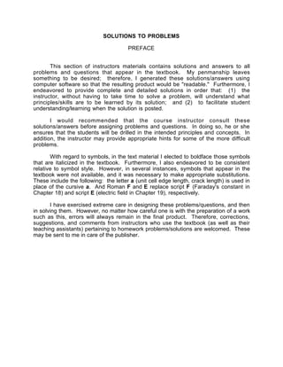
  • 5. 4 (b) Now, solving for r (= r o ) A r o 2 = nB r o (n + 1) or r o = ( ) A nB 1/(1 - n) (c) Substitution for r o into Equation (2.11) and solving for E (= E o ) E o = - A r o + B r o n = - A ( ) A nB 1/(1 - n) + B ( ) A nB n/(1 - n) 2.14 (a) Curves of E A , E R , and E N are shown on the plot below. 1.0 0.8 0.6 0.4 0.2 0.0 -7 -6 -5 -4 -3 -2 -1 0 1 2 Interatomic Separation (nm) Bonding Energy (eV) EA E R E N r o = 0.28 nm Eo = -4.6 eV
  • 6. 5 (b) From this plot r o = 0.28 nm E o = -4.6 eV (c) From Equation (2.11) for E N A = 1.436 B = 5.86 x 10 -6 n = 9 Thus, r o = ( ) A nB 1/(1 - n) =       1.436 (9)(5.86 x 10 -6 ) 1/(1 - 9) = 0.279 nm and E o = - 1.436       1.436 (9)(5.86 x 10 -6 ) 1/(1 - 9) + 5.86 x 10 -6       1.436 (9)(5.86 x 10 -6 ) 9/(1 - 9) = - 4.57 eV 2.15 This problem gives us, for a hypothetical X + -Y - ion pair, values for r o (0.35 nm), E o (-6.13 eV), and n (10), and asks that we determine explicit expressions for attractive and repulsive energies of Equations 2.8 and 2.9. In essence, it is necessary to compute the values of A and B in these equations. Expressions for r o and E o in terms of n, A, and B were determined in Problem 2.13, which are as follows: r o = ( ) A nB 1/(1 - n) E o = - A ( ) A nB 1/(1 - n) + B ( ) A nB n/(1 - n) Thus, we have two simultaneous equations with two unknowns (viz. A and B). Upon substitution of values for r o and E o in terms of n, these equations take the forms
  • 7. 6 0.35 nm = ( ) A 10B 1/(1 - 10) -6.13 eV = - A ( ) A 10B 1/(1 - 10) + B ( ) A 10B 10/(1 - 10) Simultaneous solution of these two equations leads to A = 2.38 and B = 1.88 x 10 -5 . Thus, Equations (2.8) and (2.9) become E A = - 2.38 r E R = 1.88 x 10 -5 r 10 Of course these expressions are valid for r and E in units of nanometers and electron volts, respectively. 2.16 (a) Differentiating Equation (2.12) with respect to r yields dE dr = C r 2 - De-r/ρ ρ At r = r o , dE/dr = 0, and C r 2 o = De-ro/ρ ρ (2.12b) Solving for C and substitution into Equation (2.12) yields an expression for E o as E o = De-ro/ρ       1 - r o ρ (b) Now solving for D from Equation (2.12b) above yields D = Cρe ro/ρ r o 2
  • 8. 7 Substitution of this expression for D into Equation (2.12) yields an expression for E o as E o = C r o      ρ r o - 1 2.17 (a) The main differences between the various forms of primary bonding are: Ionic--there is electrostatic attraction between oppositely charged ions. Covalent--there is electron sharing between two adjacent atoms such that each atom assumes a stable electron configuration. Metallic--the positively charged ion cores are shielded from one another, and also "glued" together by the sea of valence electrons. (b) The Pauli exclusion principle states that each electron state can hold no more than two electrons, which must have opposite spins. 2.18 Covalently bonded materials are less dense than metallic or ionically bonded ones because covalent bonds are directional in nature whereas metallic and ionic are not; when bonds are directional, the atoms cannot pack together in as dense a manner, yielding a lower mass density. 2.19 The percent ionic character is a function of the electron negativities of the ions X A and X B according to Equation (2.10). The electronegativities of the elements are found in Figure 2.7. For TiO 2 , XTi = 1.5 and X O = 3.5, and therefore, %IC = [ ] 1 - e(-0.25)(3.5 - 1.5)2 x 100 = 63.2% For ZnTe, XZn = 1.6 and XTe = 2.1, and therefore, %IC = [ ] 1 - e(-0.25)(2.1 - 1.6)2 x 100 = 6.1% For CsCl, XCs = 0.7 and XCl = 3.0, and therefore, %IC = [ ] 1 - e(-0.25)(3.0 - 0.7)2 x 100 = 73.4% For InSb, XIn = 1.7 and XSb = 1.9, and therefore,
  • 9. 8 %IC = [ ] 1 - e(-0.25)(1.9 - 1.7)2 x 100 = 1.0% For MgCl 2 , XMg = 1.2 and XCl = 3.0, and therefore, %IC = [ ] 1 - e(-0.25)(3.0 - 1.2)2 x 100 = 55.5% 2.20 Below is plotted the bonding energy versus melting temperature for these four metals. From this plot, the bonding energy for copper (melting temperature of 1084°C) should be approximately 3.6 eV. The experimental value is 3.5 eV. 4000 3000 2000 1000 0 -1000 0 2 4 6 8 10 Bonding Energy (eV) W Fe Al Hg 3.6 eV Melting Temperature (C) 2.21 For germanium, having the valence electron structure 4s 2 4p 2 , N' = 4; thus, there are 8 - N' = 4 covalent bonds per atom. For phosphorus, having the valence electron structure 3s 2 3p 3 , N' = 5; thus, there are 8 - N' = 3 covalent bonds per atom. For selenium, having the valence electron structure 4s 2 4p 4 , N' = 6; thus, there are 8 - N' = 2 covalent bonds per atom. For chlorine, having the valence electron structure 3s 2 3p 5 , N' = 7; thus, there is 8 - N' = 1 covalent bond per atom. 2.22 For brass, the bonding is metallic since it is a metal alloy. For rubber, the bonding is covalent with some van der Waals. (Rubber is composed primarily of carbon and hydrogen atoms.)
  • 10. 9 For BaS, the bonding is predominantly ionic (but with some covalent character) on the basis of the relative positions of Ba and S in the periodic table. For solid xenon, the bonding is van der Waals since xenon is an inert gas. For bronze, the bonding is metallic since it is a metal alloy (composed of copper and tin). For nylon, the bonding is covalent with perhaps some van der Waals. (Nylon is composed primarily of carbon and hydrogen.) For AlP the bonding is predominantly covalent (but with some ionic character) on the basis of the relative positions of Al and P in the periodic table. 2.23 The intermolecular bonding for HF is hydrogen, whereas for HCl, the intermolecular bonding is van der Waals. Since the hydrogen bond is stronger than van der Waals, HF will have a higher melting temperature. 2.24 The geometry of the H 2 O molecules, which are hydrogen bonded to one another, is more restricted in the solid phase than for the liquid. This results in a more open molecular structure in the solid, and a less dense solid phase.
  • 11. 10 CHAPTER 3 THE STRUCTURE OF CRYSTALLINE SOLIDS PROBLEM SOLUTIONS 3.1 Atomic structure relates to the number of protons and neutrons in the nucleus of an atom, as well as the number and probability distributions of the constituent electrons. On the other hand, crystal structure pertains to the arrangement of atoms in the crystalline solid material. 3.2 A crystal structure is described by both the geometry of, and atomic arrangements within, the unit cell, whereas a crystal system is described only in terms of the unit cell geometry. For example, face-centered cubic and body-centered cubic are crystal structures that belong to the cubic crystal system. 3.3 For this problem, we are asked to calculate the volume of a unit cell of aluminum. Aluminum has an FCC crystal structure (Table 3.1). The FCC unit cell volume may be computed from Equation (3.4) as V C = 16R 3√  2 = (16)(0.143 x 10 -9 m) 3 √  2 = 6.62 x 10 -29 m 3 3.4 This problem calls for a demonstration of the relationship a = 4R√  3 for BCC. Consider the BCC unit cell shown below a a N O P Q a Using the triangle NOP
  • 12. 11 (NP __ ) 2 = a 2 + a 2 = 2a 2 And then for triangle NPQ, (NQ __ ) 2 = (QP __ ) 2 + (NP __ ) 2 But NQ __ = 4R, R being the atomic radius. Also, QP __ = a. Therefore, (4R) 2 = a 2 + 2a 2 , or a = 4R √  3 3.5 We are asked to show that the ideal c/a ratio for HCP is 1.633. A sketch of one-third of an HCP unit cell is shown below. c a a J M K L Consider the tetrahedron labeled as JKLM, which is reconstructed as
  • 13. 12 K J L M H The atom at point M is midway between the top and bottom faces of the unit cell--that is MH __ = c/2. And, since atoms at points J, K, and M, all touch one another, JM __ = JK __ = 2R = a where R is the atomic radius. Furthermore, from triangle JHM, (JM __ ) 2 = ( JH __ ) 2 + (MH __ ) 2 , or a 2 = ( JH __ ) 2 + ( ) c 2 2 Now, we can determine the JH __ length by consideration of triangle JKL, which is an equilateral triangle, J L K H a/2 30 cos 30° = a/2 JH = √  3 2 , and JH __ = a √  3
  • 14. 13 Substituting this value for JH __ in the above expression yields a 2 =       a √  3 2 + ( ) c 2 2 = a 2 3 + c 2 4 and, solving for c/a c a = √  8 3 = 1.633 3.6 We are asked to show that the atomic packing factor for BCC is 0.68. The atomic packing factor is defined as the ratio of sphere volume to the total unit cell volume, or APF = V S V C Since there are two spheres associated with each unit cell for BCC V S = 2(sphere volume) = 2       4πR 3 3 = 8πR 3 3 Also, the unit cell has cubic symmetry, that is V C = a 3 . But a depends on R according to Equation (3.3), and V C =       4R √  3 3 = 64R 3 3√  3 Thus, APF = 8πR 3 /3 64R 3 /3√  3 = 0.68 3.7 This problem calls for a demonstration that the APF for HCP is 0.74. Again, the APF is just the total sphere-unit cell volume ratio. For HCP, there are the equivalent of six spheres per unit cell, and thus
  • 15. 14 V S = 6       4πR 3 3 = 8πR 3 Now, the unit cell volume is just the product of the base area times the cell height, c. This base area is just three times the area of the parallelepiped ACDE shown below. A B C D E a = 2R a = 2R a = 2R 60 30 The area of ACDE is just the length of CD __ times the height BC __ . But CD __ is just a or 2R, and BC __ = 2R cos(30°) = 2R√  3 2 Thus, the base area is just AREA = (3)(CD __ )(BC __ ) = (3)(2R)       2R√  3 2 = 6R 2 √  3 and since c = 1.633a = 2R(1.633) V C = (AREA)(c) = 6R 2 c√  3 = (6R 2 √  3)(2)(1.633)R = 12√  3(1.633)R 3 Thus, APF = V S V C = 8πR 3 12√  3(1.633)R 3 = 0.74 3.8 This problem calls for a computation of the density of iron. According to Equation (3.5)
  • 16. 15 ρ = nA Fe V C N A For BCC, n = 2 atoms/unit cell, and V C =       4R √  3 3 Thus, ρ = (2 atoms/unit cell)(55.9 g/mol) [ ] (4)(0.124 x 10 -7 cm) 3 /√  3 3 /(unit cell)(6.023 x 10 23 atoms/mol) = 7.90 g/cm 3 The value given inside the front cover is 7.87 g/cm 3 . 3.9 We are asked to determine the radius of an iridium atom, given that Ir has an FCC crystal structure. For FCC, n = 4 atoms/unit cell, and V C = 16R 3 √  2 [Equation (3.4)]. Now, ρ = nA Ir V C N A And solving for R from the above two expressions yields R =       nA Ir 16ρN A √  2 1/3 =       (4 atoms/unit cell)(192.2 g/mol) (√  2)(16)(22.4 g/cm 3 )(6.023 x 10 23 atoms/mol) 1/3 = 1.36 x 10 -8 cm = 0.136 nm 3.10 This problem asks for us to calculate the radius of a vanadium atom. For BCC, n = 2 atoms/unit cell, and
  • 17. 16 V C =       4R √  3 3 = 64R 3 3√  3 Since, ρ = nA V V C N A and solving for R R =       3√  3nA V 64ρN A 1/3 =         (3√  3)(2 atoms/unit cell)(50.9 g/mol) (64)(5.96 g/cm 3 )(6.023 x 10 23 atoms/mol) 1/3 = 1.32 x 10 -8 cm = 0.132 nm 3.11 For the simple cubic crystal structure, the value of n in Equation (3.5) is unity since there is only a single atom associated with each unit cell. Furthermore, for the unit cell edge length, a = 2R. Therefore, employment of Equation (3.5) yields ρ = nA V C N A = nA (2R) 3 N A = (1 atom/unit cell)(70.4 g/mol) [ ] (2)(1.26 x 10 -8 cm) 3 /unit cell(6.023 x 10 23 atoms/mol) = 7.30 g/cm 3 3.12. (a) The volume of the Zr unit cell may be computed using Equation (3.5) as V C = nA Zr ρN A Now, for HCP, n = 6 atoms/unit cell, and for Zr, A Zr = 91.2 g/mol. Thus,
  • 18. 17 V C = (6 atoms/unit cell)(91.2 g/mol) (6.51 g/cm 3 )(6.023 x 10 23 atoms/mol) = 1.396 x 10 -22 cm 3 /unit cell = 1.396 x 10 -28 m 3 /unit cell (b) From the solution to Problem 3.7, since a = 2R, then, for HCP V C = 3√  3a 2 c 2 but, since c = 1.593a V C = 3√  3(1.593)a 3 2 = 1.396 x 10 -22 cm 3 /unit cell Now, solving for a a =         (2)(1.396 x 10 -22 cm 3 ) (3)(√  3)(1.593) 1/3 = 3.23 x 10 -8 cm = 0.323 nm And finally c = 1.593a = (1.593)(0.323 nm) = 0.515 nm 3.13 This problem asks that we calculate the theoretical densities of Pb, Cr, Cu, and Co. Since Pb has an FCC crystal structure, n = 4, and V C = ( ) 2R√  2 3 . Also, R = 0.175 nm (1.75 x 10 -8 cm) and A Pb = 207.2 g/mol. Employment of Equation (3.5) yields ρ = (4 atoms/unit cell)(207.2 g/mol) [ ] (2)(1.75 x 10 -8 cm)(√  2) 3 /unit cell(6.023 x 10 23 atoms/mol) = 11.35 g/cm 3 The value given in the table inside the front cover is 11.35 g/cm 3 . Chromium has a BCC crystal structure for which n = 2 and a = 4R/√  3; also A Cr = 52.00 g/mol and R = 0.125 nm. Therefore, employment of Equation (3.5) leads to
  • 19. 18 ρ = (2 atoms/unit cell)(52.00 g/mol)         (4)(1.25 x 10 -8 cm) √  3 3 /unit cell(6.023 x 10 23 atoms/mol) = 7.18 g/cm 3 The value given in the table is 7.19 g/cm 3 . Copper has an FCC crystal structure; therefore, ρ = (4 atoms/unit cell)(63.55 g/mol) [ ] (2)(1.28 x 10 -8 cm)(√  2) 3 /unit cell(6.023 x 10 23 atoms/mol) = 8.89 g/cm 3 The value given in the table is 8.94 g/cm 3 . Cobalt has an HCP crystal structure, and from Problem 3.7, V C = 3√  3a 2 c 2 and, since c = 1.623a and a = 2R = 2(1.25 x 10 -8 cm) = 2.50 x 10 -8 cm V C = 3√  3(1.623)( ) 2.50 x 10 -8 cm 3 2 = 6.59 x 10 -23 cm 3 /unit cell Also, there are 6 atoms/unit cell for HCP. Therefore the theoretical density is ρ = nA Co V C N A = (6 atoms/unit cell)(58.93 g/mol) (6.59 x 10 -23 cm 3 /unit cell)(6.023 x 10 23 atoms/mol) = 8.91 g/cm 3
  • 20. 19 The value given in the table is 8.9 g/cm 3 . 3.14 In order to determine whether Rh has an FCC or BCC crystal structure, we need to compute its density for each of the crystal structures. For FCC, n = 4, and a = 2R√  2. Also, from Figure 2.6, its atomic weight is 102.91 g/mol. Thus, for FCC ρ = nA Rh ( ) 2R√  2 3 N A = (4 atoms/unit cell)(102.91 g/mol) [ ] (2)(1.345 x 10 -8 cm)(√  2) 3 /unit cell(6.023 x 10 23 atoms/mol) = 12.41 g/cm 3 which is the value provided in the problem. Therefore, Rh has an FCC crystal structure. 3.15 For each of these three alloys we need to, by trial and error, calculate the density using Equation (3.5), and compare it to the value cited in the problem. For SC, BCC, and FCC crystal structures, the respective values of n are 1, 2, and 4, whereas the expressions for a (since V C = a 3 ) are 2R, 2R√  2, and 4R/√  3. For alloy A, let us calculate ρ assuming a simple cubic crystal structure. ρ = nA A V C N A = (1 atom/unit cell)(77.4 g/mol) [ ] (2)(1.25 x 10 -8 cm) 3 /unit cell(6.023 x 10 23 atoms/mol) = 8.22 g/cm 3 Therefore, its crystal structure is SC. For alloy B, let us calculate ρ assuming an FCC crystal structure. ρ = (4 atoms/unit cell)(107.6 g/mol) [ ] (2)√  2(1.33 x 10 -8 cm) 3 /unit cell(6.023 x 10 23 atoms/mol)
  • 21. 20 = 13.42 g/cm 3 Therefore, its crystal structure is FCC. For alloy C, let us calculate ρ assuming an SC crystal structure. ρ = (1 atom/unit cell)(127.3 g/mol) [ ] (2)(1.42 x 10 -8 cm) 3 /unit cell(6.023 x 10 23 atoms/mol) = 9.23 g/cm 3 Therefore, its crystal structure is SC. 3.16 In order to determine the APF for Sn, we need to compute both the unit cell volume (V C ) which is just the a 2 c product, as well as the total sphere volume (V S ) which is just the product of the volume of a single sphere and the number of spheres in the unit cell (n). The value of n may be calculated from Equation (3.5) as n = ρV C N A A Sn = (7.30)(5.83) 2 (3.18)(x 10 -24 )(6.023 x 10 23 ) 118.69 = 4.00 atoms/unit cell Therefore APF = V S V C = (4)( ) 4 3 πR 3 (a) 2 (c) (4)[ ] 4 3 (π)(0.151) 3 (0.583) 2 (0.318) = 0.534 3.17 (a) From the definition of the APF
  • 22. 21 APF = V S V C = n( ) 4 3 πR 3 abc we may solve for the number of atoms per unit cell, n, as n = (APF)abc 4 3 πR 3 = (0.547)(4.79)(7.25)(9.78)(10 -24 cm 3 ) 4 3 π(1.77 x 10 -8 cm) 3 = 8.0 atoms/unit cell (b) In order to compute the density, we just employ Equation (3.5) as ρ = nA I abcN A = (8 atoms/unit cell)(126.91 g/mol) [ ] (4.79)(7.25)(9.78) x 10 -24 cm 3 /unit cell (6.023 x 10 23 atoms/mol) = 4.96 g/cm 3 3. 18 (a) We are asked to calculate the unit cell volume for Ti. From the solution to Problem 3.7 V C = 6R 2 c√  3 But, c = 1.58a, and a = 2R, or c = 3.16R, and V C = (6)(3.16)R 3 √  3 = (6)(3.16)(√  3)[ ] 0.1445 x 10 -7 cm 3 = 9.91 x 10 -23 cm 3 /unit cell (b) The density of Ti is determined as follows:
  • 23. 22 ρ = nA Ti V C N A For HCP, n = 6 atoms/unit cell, and for Ti, A Ti = 47.88 g/mol. Thus, ρ = (6 atoms/unit cell)(47.88 g/mol) (9.91 x 10 -23 cm 3 /unit cell)(6.023 x 10 23 atoms/mol) = 4.81 g/cm 3 The value given in the literature is 4.51 g/cm 3 . 3.19 This problem calls for us to compute the atomic radius for Zn. In order to do this we must use Equation (3.5), as well as the expression which relates the atomic radius to the unit cell volume for HCP; from Problem 3.7 it was shown that V C = 6R 2 c√  3 In this case c = 1.856(2R). Making this substitution into the previous equation, and then solving for R using Equation (3.5) yields R =         nA Zn (1.856)(12√  3)ρN A 1/3 =       (6 atoms/unit cell)(65.39 g/mol) (1.856)(12√  3)(7.13 g/cm 3 )(6.023 x 10 23 atoms/mol) 1/3 = 1.33 x 10 -8 cm = 0.133 nm 3.20 This problem asks that we calculate the unit cell volume for Re which has an HCP crystal structure. In order to do this, it is necessary to use a result of Problem 3.7, that is V C = 6R 2 c√  3 The problem states that c = 1.615a, and a = 2R. Therefore
  • 24. 23 V C = (1.615)(12√  3)R 3 = (1.615)(12√  3)(1.37 x 10 -8 cm) 3 = 8.63 x 10 -23 cm 3 = 8.63 x 10 -2 nm 3 3.21 (a) The unit cell shown in the problem belongs to the tetragonal crystal system since a = b = 0.30 nm, c = 0.40 nm, and α = β = γ = 90°. (b) The crystal structure would be called body-centered tetragonal. (c) As with BCC n = 2 atoms/unit cell. Also, for this unit cell V C = (3.0 x 10 -8 cm) 2 (4.0 x 10 -8 cm) = 3.60 x 10 -23 cm 3 /unit cell Thus, ρ = nA V C N A = (2 atoms/unit cell)(141 g/mol) (3.60 x 10 -23 cm 3 /unit cell)(6.023 x 10 23 atoms/mol) = 13.0 g/cm 3 3.22 The unit cell for AuCu 3 is to be generated using the software found on the CD-ROM. 3.23 The unit cell for AuCu is to be generated using the software found on the CD-ROM. 3.24 A unit cell for the body-centered orthorhombic crystal structure is presented below. b 90 90 90 a c
  • 25. 24 3.25 (a) This portion of the problem calls for us to draw a [121 _ ] direction within an orthorhombic unit cell (a ≠ b ≠ c, α = β = γ = 90°). Such a unit cell with its origin positioned at point O is shown below. We first move along the +x-axis a units (from point O to point A), then parallel to the +y- axis 2b units (from point A to point B). Finally, we proceed parallel to the z-axis -c units (from point B to point C). The [121 _ ] direction is the vector from the origin (point O) to point C as shown. b 90 90 90 c a x y z O A B C (b) We are now asked to draw a (210) plane within an orthorhombic unit cell. First remove the three indices from the parentheses, and take their reciprocals--i.e., 1/2, 1, and ∞. This means that the plane intercepts the x-axis at a/2, the y-axis at b, and parallels the z-axis. The plane that satisfies these requirements has been drawn within the orthorhombic unit cell below.
  • 26. 25 b c a x y z 3.26 (a) This portion of the problem asks that a [01 _ 1] direction be drawn within a monoclinic unit cell (a ≠ b ≠ c, and α = β = 90° ≠ γ). One such unit cell with its origin at point O is sketched below. For this direction, there is no projection along the x-axis since the first index is zero; thus, the direction lies in the y-z plane. We next move from the origin along the minus y-axis b units (from point O to point R). Since the final index is a one, move from point R parallel to the z-axis, c units (to point P). Thus, the [01 _ 1] direction corresponds to the vector passing from the origin to point P, as indicated in the figure. x y z a b c α β γ O -y R P [011] - (b) A (002) plane is drawn within the monoclinic cell shown below. We first remove the parentheses and take the reciprocals of the indices; this gives ∞, ∞, and 1/2. Thus, the (002) plane parallels both x- and y-axes, and intercepts the z-axis at c/2, as indicated in the drawing.
  • 27. 26 x y z a b c α β γ O 3.27 (a) We are asked for the indices of the two directions sketched in the figure. For direction 1, the projection on the x-axis is zero (since it lies in the y-z plane), while projections on the y- and z-axes are b/2 and c, respectively. This is an [012] direction as indicated in the summary below x y z Projections 0a b/2 c Projections in terms of a, b, and c 0 1/2 1 Reduction to integers 0 1 2 Enclosure [012] Direction 2 is [112 _ ] as summarized below. x y z Projections a/2 b/2 -c Projections in terms of a, b, and c 1/2 1/2 -1 Reduction to integers 1 1 -2 Enclosure [112 _ ]
  • 28. 27 (b) This part of the problem calls for the indices of the two planes which are drawn in the sketch. Plane 1 is an (020) plane. The determination of its indices is summarized below. x y z Intercepts ∞ a b/2 ∞ c Intercepts in terms of a, b, and c ∞ 1/2 ∞ Reciprocals of intercepts 0 2 0 Enclosure (020) Plane 2 is a (22 _ 1) plane, as summarized below. x y z Intercepts a/2 -b/2 c Intercepts in terms of a, b, and c 1/2 -1/2 1 Reciprocals of intercepts 2 -2 1 Enclosure (22 _ 1) 3.28 The directions asked for are indicated in the cubic unit cells shown below.
  • 30. 29 z y x [103] _ [133] _ [111] __ [122] _ 3.29 Direction A is a [01 _ 1 _ ] direction, which determination is summarized as follows. We first of all position the origin of the coordinate system at the tail of the direction vector; then in terms of this new coordinate system x y z Projections 0a -b -c Projections in terms of a, b, and c 0 -1 -1 Reduction to integers not necessary Enclosure [01 _ 1 _ ] Direction B is a [2 _ 10] direction, which determination is summarized as follows. We first of all position the origin of the coordinate system at the tail of the direction vector; then in terms of this new coordinate system x y z Projections -a b 2 0c Projections in terms of a, b, and c -1 1 2 0 Reduction to integers -2 1 0 Enclosure [2 _ 10]
  • 31. 30 Direction C is a [112] direction, which determination is summarized as follows. We first of all position the origin of the coordinate system at the tail of the direction vector; then in terms of this new coordinate system x y z Projections a 2 b 2 c Projections in terms of a, b, and c 1 2 1 2 1 Reduction to integers 1 1 2 Enclosure [112] Direction D is a [112 _ ] direction, which determination is summarized as follows. We first of all position the origin of the coordinate system at the tail of the direction vector; then in terms of this new coordinate system x y z Projections a 2 b 2 -c Projections in terms of a, b, and c 1 2 1 2 -1 Reduction to integers 1 1 -2 Enclosure [112 _ ] 3.30 Direction A is a [4 _ 30] direction, which determination is summarized as follows. We first of all position the origin of the coordinate system at the tail of the direction vector; then in terms of this new coordinate system x y z Projections - 2a 3 b 2 0c Projections in terms of a, b, and c - 2 3 1 2 0
  • 32. 31 Reduction to integers -4 3 0 Enclosure [4 _ 30] Direction B is a [23 _ 2] direction, which determination is summarized as follows. We first of all position the origin of the coordinate system at the tail of the direction vector; then in terms of this new coordinate system x y z Projections 2a 3 -b 2c 3 Projections in terms of a, b, and c 2 3 -1 2 3 Reduction to integers 2 -3 2 Enclosure [23 _ 2] Direction C is a [13 _ 3 _ ] direction, which determination is summarized as follows. We first of all position the origin of the coordinate system at the tail of the direction vector; then in terms of this new coordinate system x y z Projections a 3 -b -c Projections in terms of a, b, and c 1 3 -1 -1 Reduction to integers 1 -3 -3 Enclosure [13 _ 3 _ ] Direction D is a [136 _ ] direction, which determination is summarized as follows. We first of all position the origin of the coordinate system at the tail of the direction vector; then in terms of this new coordinate system
  • 33. 32 x y z Projections a 6 b 2 -c Projections in terms of a, b, and c 1 6 1 2 -1 Reduction to integers 1 3 -6 Enclosure [136 _ ] 3.31 For tetragonal crystals a = b ≠ c and α = β = γ = 90°; therefore, projections along the x and y axes are equivalent, which are not equivalent to projections along the z axis. (a) Therefore, for the [101] direction, equivalent directions are the following: [1 _ 01 _ ], [1 _ 01], [101 _ ], [011], [011 _ ], [01 _ 1], [01 _ 1 _ ]. (b) For the [110] direction, equivalent directions are the following: [1 _ 1 _ 0], [1 _ 10], and [11 _ 0]. (c) For the [010] direction, equivalent directions are the following: [01 _ 0], [100], and [1 _ 00] 3.32 (a) We are asked to convert [100] and [111] directions into the four- index Miller-Bravais scheme for hexagonal unit cells. For [100] u' = 1, v' = 0, w' = 0 From Equations (3.6) u = n 3 (2u' - v') = n 3 (2 - 0) = 2n 3 v = n 3 (2v' - u') = n 3 (0 - 1) = - n 3 t = - (u + v) = - ( ) 2n 3 - n 3 = - n 3 w = nw' = 0
  • 34. 33 If we let n = 3, then u = 2, v = -1, t = -1, and w = 0. Thus, the direction is represented as [uvtw] = [211 __ 0]. For [111], u' = 1, v' = 1, and w' = 1; therefore, u = n 3 (2 - 1) = n 3 v = n 3 (2 - 1) = n 3 t = - ( ) n 3 + n 3 = - 2n 3 w = n If we again let n = 3, then u = 1, v = 1, t = -2, and w = 3. Thus, the direction is represented as [112 _ 3]. (b) This portion of the problem asks for the same conversion of the (010) and (101) planes. A plane for hexagonal is represented by (hkil) where i = - (h + k), and h, k, and l are the same for both systems. For the (010) plane, h = 0, k = 1, l = 0, and i = - (0 + 1) = -1 Thus, the plane is now represented as (hkil) = (011 _ 0). For the (101) plane, i = - (1 + 0) = -1, and (hkil) = (101 _ 1). 3.33 For plane A we will leave the origin at the unit cell as shown; this is a (403) plane, as summarized below. x y z Intercepts a 2 ∞b 2c 3 Intercepts in terms of a, b, and c 1 2 ∞ 2 3
  • 35. 34 Reciprocals of intercepts 2 0 3 2 Reduction 4 0 3 Enclosure (403) For plane B we will move the origin of the unit cell one unit cell distance to the right along the y axis, and one unit cell distance parallel to the x axis; thus, this is a (1 _ 1 _ 2) plane, as summarized below. x y z Intercepts -a -b c 2 Intercepts in terms of a, b, and c -1 -1 1 2 Reciprocals of intercepts -1 -1 2 Enclosure (1 _ 1 _ 2) 3.34 For plane A we will move the origin of the coordinate system one unit cell distance to the upward along the z axis; thus, this is a (322 _ ) plane, as summarized below. x y z Intercepts a 3 b 2 - c 2 Intercepts in terms of a, b, and c 1 3 1 2 - 1 2 Reciprocals of intercepts 3 2 -2 Enclosure (322 _ ) For plane B we will move the original of the coordinate system on unit cell distance along the x axis; thus, this is a (1 _ 01) plane, as summarized below. x y z Intercepts - a 2 ∞b c 2
  • 36. 35 Intercepts in terms of a, b, and c - 1 2 ∞ 1 2 Reciprocals of intercepts -2 0 2 Reduction -1 0 1 Enclosure (1 _ 01) 3.35 For plane A since the plane passes through the origin of the coordinate system as shown, we will move the origin of the coordinate system one unit cell distance to the right along the y axis; thus, this is a (32 _ 4) plane, as summarized below. x y z Intercepts 2a 3 -b c 2 Intercepts in terms of a, b, and c 2 3 -1 1 2 Reciprocals of intercepts 3 2 -1 2 Reduction 3 -2 4 Enclosure (32 _ 4) For plane B we will leave the origin at the unit cell as shown; this is a (221) plane, as summarized below. x y z Intercepts a 2 b 2 c Intercepts in terms of a, b, and c 1 2 1 2 1 Reciprocals of intercepts 2 2 1 Enclosure (221) 3.36 The (11 _ 01) and (112 _ 0) planes in a hexagonal unit cell are shown below.
  • 37. 36 z a 1 a 2 a 3 z a 1 a 2 a 3 (1101) _ (1120) _ 3.37 (a) For this plane we will leave the origin of the coordinate system as shown; thus, this is a (11 _ 00) plane, as summarized below. a 1 a 2 a 3 z Intercepts a - a ∞a ∞c Intercepts in terms of a's and c 1 -1 ∞ ∞ Reciprocals of intercepts 1 -1 0 0 Enclosure (11 _ 00) (b) For this plane we will leave the origin of the coordinate system as shown; thus, this is a (211 __ 2) plane, as summarized below. a 1 a 2 a 3 z Intercepts a 2 -a -a c 2 Intercepts in terms of a's and c 1 2 -1 -1 1 2 Reciprocals of intercepts 2 -1 -1 2 Enclosure (211 __ 2) 3.38 The planes called for are plotted in the cubic unit cells shown below.
  • 38. 37 x y z (131) _ (112) _ (102) _ z x y (011) __ x y z (111) _ _ _ (122) _ x y z _ (013) _ _ (123) _ 3.39 (a) The atomic packing of the (100) plane for the FCC crystal structure is called for. An FCC unit cell, its (100) plane, and the atomic packing of this plane are indicated below. (100) Plane
  • 39. 38 (b) For this part of the problem we are to show the atomic packing of the (111) plane for the BCC crystal structure. A BCC unit cell, its (111) plane, and the atomic packing of this plane are indicated below. Plane (111) 3.40 (a) The unit cell in Problem 3.21 is body-centered tetragonal. Only the (100) (front face) and (01 _ 0) (left side face) planes are equivalent since the dimensions of these planes within the unit cell (and therefore the distances between adjacent atoms) are the same (namely 0.40 nm x 0.30 nm), which are different than the (001) (top face) plane (namely 0.30 nm x 0.30 nm). (b) The (101) and (011) planes are equivalent; their dimensions within the unit cell are the same--that is 0.30 nm x [ ] (0.30 nm) 2 + (0.40 nm) 2 1/2 . Furthermore, the (110) and (1 _ 10) planes are equivalent; the dimensions of these planes within a unit cell are the same--that is 0.40 nm x [ ] (0.30 nm) 2 + (0.30 nm) 2 1/2 . (c) All of the (111), (11 _ 1), (111 _ ), and (1 _ 11 _ ) planes are equivalent. 3.41 (a) The intersection between (110) and (111) planes results in a [1 _ 10], or equivalently, a [11 _ 0] direction. (b) The intersection between (110) and (11 _ 0) planes results in a [001], or equivalently, a [001 _ ] direction. (c) The intersection between (101 _ ) and (001) planes results in a [010], or equivalently, a [01 _ 0] direction. 3.42 For FCC the linear density of the [100] direction is computed as follows: The linear density, LD, is defined by the ratio LD = L c L l
  • 40. 39 where L l is the line length within the unit cell along the [100] direction, and L c is line length passing through intersection circles. Now, L l is just the unit cell edge length, a which, for FCC is related to the atomic radius R according to a = 2R√  2 [Equation (3.1)]. Also for this situation, L c = 2R and therefore LD = 2R 2R√  2 = 0.71 For the [110] direction, L l = L c = 4R and therefore, LD = 4R 4R = 1.0 For the [111] direction L c = 2R, whereas L l = 2R√  6, therefore LD = 2R 2R√  6 = 0.41 3.43 The linear density, LD, is the ratio of L c and L l . For the [110] direction in BCC, L c = 2R, whereas L l = 4R√  2 √  3 . Therefore LD = L c L l = 2R 4R√  2 √  3 = 0.61 For the [111] direction in BCC, L c = L l = 4R; therefore LD = 4R 4R = 1.0 3.44 Planar density, PD, is defined as PD = A c A p where A p is the total plane area within the unit cell and A c is the circle plane area within this same plane. For the (100) plane in FCC, in terms of the atomic radius, R, and the unit cell edge length a
  • 41. 40 A p = a 2 = ( ) 2R√  2 2 = 8R 2 Also, upon examination of that portion of the (100) plane within a single unit cell, it may be noted that there reside 2 equivalent atoms--one from the center atom, and one-fourth of each of the four corner atoms. Therefore, A c = (2)πR 2 Hence PD = 2πR 2 8R 2 = 0.79 That portion of a (111) plane that passes through a FCC unit cell forms a triangle as shown below. 4R R 2R 3 In terms of the atomic radius R, the length of the triangle base is 4R, whereas the height is 2R√  3. Therefore, the area of this triangle, which is just A p is A p = 1 2 (4R)(2R√  3) = 4R 2 √  3 Now it becomes necessary to determine the number of equivalent atoms residing within this plane. One-sixth of each corner atom and one-half of each middle atom belong belongs to the unit cell. Therefore, since there are 3 corner and 3 middle atoms, there is an equivalent of 2 atoms within the unit cell. Hence A c = 2(πR 2 )
  • 42. 41 and PD = 2πR 2 4R 2 √  3 = 0.91 3.45 Planar density, PD, is defined as PD = A c A p where A p is the total plane area within the unit cell and A c is the circle plane area within this same plane. For the (100) plane in BCC, in terms of the atomic radius, R, and the unit cell edge length a A p = a 2 =       4R √  3 2 = 16R 2 3 Also, upon examination of that portion of the (100) plane within a single unit cell, that there resides a single equivalent atom--one-fourth from each of the four corner atoms. Therefore, A c = πR 2 Hence PD = πR 2 16R 2 3 = 0.59 That portion of a (110) plane that passes through a BCC unit cell forms a rectangle as shown below.
  • 43. 42 3 4R R 3 2 4R In terms of the atomic radius R, the length of the rectangle base is 4R√  2/√  3, whereas the height is a = 4R √  3 . Therefore, the area of this rectangle, which is just A p is A p =       4R√  2 √  3       4R √  3 = 16R 2 √  2 3 Now for the number equivalent atoms within this plane. One-fourth of each corner atom and the entirety of the center atom belong to the unit cell. Therefore, there is an equivalent of 2 atoms within the unit cell. Hence A c = 2(πR 2 ) and PD = 2πR 2 16R 2 √  2 3 = 0.83 3.46 Below is shown portion of a (0001) plane for HCP. Also indicated is a hexagon corresponding to the base of one unit cell which consists of six equilateral triangles.
  • 44. 43 2R In terms of the atomic radius R, the area of each triangle is R 2 √  3, or the total area A p is just 6R 2 √  3. Now, the entirety of the center circle lies within this hexagon, as well as and one-third of each of the six corner circles; thus there are 3 equivalent circles associated with the hexagon, and therefore, A c = (3)πR 2 Thus, the planar density is just PD = A c A p = 3πR 2 6R 2 √  3 = 0.91 3.47 Below is constructed a unit cell using the six crystallographic directions that were provided in the problem. x z y [001] (0.50 nm) [100] (0.40 nm) [010] (0.40 nm) [110] (0.566 nm) [011] (0.64 nm) [101] (0.64 nm) (a) This unit cell belongs to the tetragonal crystal system since a = b = 0.40 nm, c = 0.50 nm, and α = β = γ = 90°.
  • 45. 44 (b) This crystal structure would be called face-centered tetragonal since the unit cell has tetragonal symmetry, and an atom is located at each of the corners, as well as at the centers of all six unit cell faces. In the figure above, atoms are only shown at the centers of three faces; however, atoms would also be situated at opposite faces. 3.48 The unit cell is constructed below from the three crystallographic planes that were provided in the problem. x y z 0.40nm 0.30nm 0.35nm (001) (110) (101) (a) This unit cell belongs to the orthorhombic crystal system since a = 0.30 nm, b = 0.40 nm, c = 0.35 nm, and α = β = γ = 90°. (b) This crystal structure would be called body-centered orthorhombic since the unit cell has orthorhombic symmetry, and an atom is located at each of the corners, as well as at the cell center. (c) In order to compute its atomic weight, we employ Equation (3.5), with n = 2; thus A = ρV C N A n = (8.95 g/cm 3 )(3.0)(4.0)(3.5)(x 10 -24 cm 3 /unit cell)(6.023 x 10 23 atoms/mol) 2 atoms/unit cell = 113.2 g/mol 3.49 Although each individual grain in a polycrystalline material may be anisotropic, if the grains have random orientations, then the solid aggregate of the many anisotropic grains will behave isotropically.
  • 46. 45 3.50 From the table, molybdenum has a BCC crystal structure and an atomic radius of 0.1363 nm. Using Equation (3.3), the lattice parameter a may be computed as a = 4R √  3 = (4)(0.1363 nm) √  3 = 0.3148 nm Now, the interplanar spacing d 111 maybe determined using Equation (3.10) as d 111 = a √  (1) 2 + (1) 2 + (1) 2 = 0.3148 √  3 = 0.1818 nm 3.51 We must first calculate the lattice parameter using Equation (3.1) and the value of R cited in Table 3.1 as a = 2R√  2 = (2)(0.1387 nm)√  2 = 0.3923 nm Next, the interplanar spacing may be determined using Equation (3.10) according to d 113 = a √  (1) 2 + (1) 2 + (3) 2 = 0.3923 nm √  11 = 0.1183 nm And finally, employment of Equation (3.9) yields sin θ = nλ 2d = (1)(0.1542 nm) (2)(0.1183 nm) = 0.652 θ = sin -1 (0.652) = 40.69° And 2θ = (2)(40.69°) = 81.38° 3.52 From the table, aluminum has an FCC crystal structure and an atomic radius of 0.1431 nm. Using Equation (3.1) the lattice parameter, a, may be computed as a = 2R√  2 = (2)(0.1431 nm)(√  2) = 0.4047 nm Now, the d 110 interplanar spacing may be determined using Equation (3.10) as
  • 47. 46 d 110 = a √  (1) 2 + (1) 2 + (0) 2 = 0.4047 nm √  2 = 0.2862 nm And, similarly for d 221 d 221 = a √  (2) 2 + (2) 2 + (1) 2 = 0.4047 nm √  9 = 0.1349 nm 3.53 (a) From the data given in the problem, and realizing that 69.22° = 2θ, the interplanar spacing for the (220) set of planes may be computed using Equation (3.9) as d 220 = nλ 2 sin θ = (1)(0.1542 nm) (2)( ) sin 69.22° 2 = 0.1357 nm (b) In order to compute the atomic radius we must first determine the lattice parameter, a using Equation (3.10), and then R from Equation (3.1) since Ir has a FCC crystal structure. Therefore, a = d 220 √  (2) 2 + (2) 2 + (0) 2 = (0.1357 nm)(√  8) = 0.3838 nm And R = a 2√  2 = 0.3838 nm 2√  2 = 0.1357 nm 3.54 (a) From the data given in the problem, and realizing that 27.00° = 2θ, the interplanar spacing for the (321) set of planes may be computed using Equation (3.9) as d 321 = nλ 2 sin θ = (1)(0.0711 nm) (2)( ) sin 27.00° 2 = 0.1523 nm (b) In order to compute the atomic radius we must first determine the lattice parameter, a using Equation (3.10), and then R from Equation (3.3) since Rb has a BCC crystal structure. Therefore, a = d 321 √  (3) 2 + (2) 2 + (1) 2 = (0.1523 nm)(√  14) = 0.5700 nm And
  • 48. 47 R = a√  3 4 = (0.5700 nm)√  3 4 = 0.2468 nm 3.55 The first step to solve this problem is to compute the interplanar spacing using Equation (3.9). Thus, d hkl = nλ 2 sin θ = (1)(0.0711 nm) (2)( ) sin 46.21° 2 = 0.0906 nm Now, employment of both Equations (3.10) and (3.3), and the value of R for iron from Table 3.1 (0.1241 nm) leads to √  h 2 + k 2 + l 2 = a d hkl = 4R d hkl √  3 = (4)(0.1241 nm) (0.0906 nm)√  3 = 3.163 This means that h 2 + k 2 + l 2 = (3.163) 2 = 10.0 By trial and error, the only three integers having a sum that is even, and the sum of the squares of which equals 10.0 are 3, 1, and 0. Therefore, the set of planes responsible for this diffraction peak are the (310) ones. 3.56 For each peak, in order to compute the interplanar spacing and the lattice parameter we must employ Equations (3.10) and (3.9), respectively. For the first peak which occurs at 45.0° d 110 = nλ 2 sin θ = (1)(0.1542 nm) (2)( ) sin 45.0° 2 = 0.2015 nm And a = d hkl √  (h) 2 + (k) 2 + (l) 2 = d 110 √  (1) 2 + (1) 2 + (0) 2
  • 49. 48 = (0.2015 nm)√  2 = 0.2850 nm Similar computations are made for the other peaks which results are tabulated below: Peak Index 2θ d hkl (nm) a (nm) 200 65.1 0.1433 0.2866 211 82.8 0.1166 0.2856 3.57 The first four diffraction peaks that will occur for FCC consistent with h, k, and l all being odd or even are (111), (200), (220), and (311). 3.58 (a) Since Cu has an FCC crystal structure, only those peaks for which h, k, and l are all either odd or even will appear. Therefore, the first peak results by diffraction from (111) planes. (b) For each peak, in order to calculate the interplanar spacing we must employ Equation (3.9). For the first peak which occurs at 43.8° d 111 = nλ 2 sin θ = (1)(0.1542 nm) (2)( ) sin 43.8° 2 = 0.2067 nm (c) Employment of Equations (3.10) and (3.1) is necessary for the computation of R for Cu as R = a 2√  2 = (d hkl )√  (h) 2 + (k) 2 + (l) 2 2√  2 = (0.2067 nm)√  (1) 2 + (1) 2 + (1) 2 2√  2 = 0.1266 nm Similar computations are made for the other peaks which results are tabulated below: Peak Index 2θ d hkl (nm) R (nm) 200 50.8 0.1797 0.1271 220 74.4 0.1275 0.1275 311 90.4 0.1087 0.1274
  • 50. 49 The value cited in Table 3.1 is 0.1278 nm, which is relatively close to these values. 3.59 A material in which atomic bonding is predominantly ionic in nature is less likely to form a noncrystalline solid upon solidification than a covalent material because covalent bonds are directional whereas ionic bonds are nondirectional; it is more difficult for the atoms in a covalent material to assume positions giving rise to an ordered structure.
  • 51. 48 CHAPTER 4 IMPERFECTIONS IN SOLIDS PROBLEM SOLUTIONS 4.1 In order to compute the fraction of atom sites that are vacant in lead at 600 K, we must employ Equation (4.1). As stated in the problem, Q v = 0.55 eV/atom. Thus, N V N = exp       - Q V kT = exp       - 0.55 eV/atom (8.62 x 10 -5 eV/atom-K)(600 K) = 2.41 x 10 -5 4.2 Determination of the number of vacancies per cubic meter in iron at 850°C (1123 K) requires the utilization of Equations (4.1) and (4.2) as follows: N V = N exp       - Q V kT = N A ρ Fe A Fe exp       - Q V kT = (6.023 x 10 23 atoms/mol)(7.65 g/cm 3 ) 55.85 g/mol exp       - 1.08 eV/atom (8.62 x 10 -5 eV/atom-K)(1123 K) = 1.18 x 10 18 cm -3 = 1.18 x 10 24 m -3 4.3 This problem calls for the computation of the activation energy for vacancy formation in silver. Upon examination of Equation (4.1), all parameters besides Q v are given except N, the total number of atomic sites. However, N is related to the density, (ρ), Avogadro's number (N A ), and the atomic weight (A) according to Equation (4.2) as N = N A ρ Pb A Pb = (6.023 x 10 23 atoms/mol)(9.5 g/cm 3 ) 107.9 g/mol = 5.30 x 10 22 atoms/cm 3 = 5.30 x 10 28 atoms/m 3
  • 52. 49 Now, taking natural logarithms of both sides of Equation (4.1), and, after some algebraic manipulation Q V = - RT ln       N V N = - (8.62 x 10 -5 eV/atom-K)(1073 K) ln         3.60 x 10 23 m -3 5.30 x 10 28 m -3 = 1.10 eV/atom 4.4 In this problem we are asked to cite which of the elements listed form with Cu the three possible solid solution types. For complete substitutional solubility the following criteria must be met: 1) the difference in atomic radii between Ni and the other element (∆R%) must be less than ±15%, 2) the crystal structures must be the same, 3) the electronegativities must be similar, and 4) the valences should be the same, or nearly the same. Below are tabulated, for the various elements, these criteria. Crystal ∆Electro- Element ∆R% Structure negativity Valence Cu FCC 2+ C -44 H -64 O -53 Ag +13 FCC 0 1+ Al +12 FCC -0.4 3+ Co -2 HCP -0.1 2+ Cr -2 BCC -0.3 3+ Fe -3 BCC -0.1 2+ Ni -3 FCC -0.1 2+ Pd +8 FCC +0.3 2+ Pt +9 FCC +0.3 2+ Zn +4 HCP -0.3 2+
  • 53. 50 (a) Ni, Pd, and Pt meet all of the criteria and thus form substitutional solid solutions having complete solubility. (b) Ag, Al, Co, Cr, Fe, and Zn form substitutional solid solutions of incomplete solubility. All these metals have either BCC or HCP crystal structures, and/or the difference between their atomic radii and that for Ni are greater than ±15%, and/or have a valence different than 2+. (c) C, H, and O form interstitial solid solutions. These elements have atomic radii that are significantly smaller than the atomic radius of Cu. 4.5 In the drawing below is shown the atoms on the (100) face of a FCC unit cell; the interstitial site is at the center of the edge. R R 2r a The diameter of an atom that will just fit into this site (2r) is just the difference between that unit cell edge length (a) and the radii of the two host atoms that are located on either side of the site (R); that is 2r = a - 2R However, for FCC a is related to R according to Equation (3.1) as a = 2R√  2; therefore, solving for r gives r = a - 2R 2 = 2R√  2 - 2R 2 = 0.41R A (100) face of a BCC unit cell is shown below.
  • 54. 51 R R + r a/4 a/2 The interstitial atom that just fits into this interstitial site is shown by the small circle. It is situated in the plane of this (100) face, midway between the two vertical unit cell edges, and one quarter of the distance between the bottom and top cell edges. From the right triangle that is defined by the three arrows we may write ( ) a 2 2 + ( ) a 4 2 = ( ) R + r 2 However, from Equation (3.3), a = 4R √  3 , and, therefore, the above equation takes the form       4R 2√  3 2 +       4R 4√  3 2 = R 2 + 2Rr + r 2 After rearrangement the following quadratic equation results: r 2 + 2Rr - 0.667R 2 = 0 And upon solving for r, r = 0.291R. Thus, for a host atom of radius R, the size of an interstitial site for FCC is approximately 1.4 times that for BCC.
  • 55. 52 4.6 (a) This problem asks that we derive Equation (4.7a). To begin, C 1 is defined according to Equation (4.3) as C 1 = m 1 m 1 + m 2 x 100 or, equivalently C 1 = m ' 1 m ' 1 + m ' 2 x 100 where the primed m's indicate masses in grams. From Equation (4.4) we may write m ' 1 = n m1 A 1 m ' 2 = n m2 A 2 And, substitution into the C 1 expression C 1 = n m1 A 1 n m1 A 1 + n m2 A 2 x 100 From Equation (4.5) it is the case that n m1 = C ' 1 (n m1 + n m2 ) 100 n m2 = C ' 2 (n m1 + n m2 ) 100 And substitution of these expressions into the above equation leads to C 1 = C ' 1 A 1 C ' 1 A 1 + C ' 2 A 2 x 100 which is just Equation (4.7a).
  • 56. 53 (b) This problem asks that we derive Equation (4.9a). To begin, C" 1 is defined as the mass of component 1 per unit volume of alloy, or C" 1 = m 1 V If we assume that the total alloy volume V is equal to the sum of the volumes of the two constituents--i.e., V = V 1 + V 2 --then C" 1 = m 1 V 1 + V 2 Furthermore, the volume of each constituent is related to its density and mass as V 1 = m 1 ρ 1 V 2 = m 2 ρ 2 This leads to C" 1 = m 1 m 1 ρ 1 + m 2 ρ 2 From Equation (4.3), m 1 and m 2 may be expressed as follows: m 1 = C 1 (m 1 + m 2 ) 100 m 2 = C 2 (m 1 + m 2 ) 100 Substitution of these equations into the preceding expression yields
  • 57. 54 C" 1 = C 1 (m 1 + m 2 ) 100 C 1 (m 1 + m 2 ) 100 ρ 1 + C 2 (m 1 + m 2 ) 100 ρ 2 = C 1 C 1 ρ 1 + C 2 ρ 2 If the densities ρ 1 and ρ 2 are given in units of g/cm 3 , then conversion to units of kg/m 3 requires that we multiply this equation by 10 3 , inasmuch as 1 g/cm 3 = 10 3 kg/m 3 Therefore, the previous equation takes the form C" 1 =           C 1 C 1 ρ 1 + C 2 ρ 2 x 10 3 which is the desired expression. (c) Now we are asked to derive Equation (4.10a). The density of an alloy ρ ave is just the total alloy mass M divided by its volume V ρ ave = M V Or, in terms of the component elements 1 and 2 ρ ave = m 1 + m 2 V 1 + V 2 Here it is assumed that the total alloy volume is equal to the separate volumes of the individual components, which is only an approximation; normally V will not be exactly equal to (V 1 + V 2 ).
  • 58. 55 Each of V 1 and V 2 may be expressed in terms of its mass density, which when substituted into the above equation ρ ave = m 1 + m 2 m 1 ρ 1 + m 2 ρ 2 Furthermore, from Equation (4.3) m 1 = C 1 (m 1 + m 2 ) 100 m 2 = C 2 (m 1 + m 2 ) 100 Which, when substituted into the above ρ ave expression yields ρ ave = m 1 + m 2 C 1 (m 1 + m 2 ) 100 ρ 1 + C 2 (m 1 + m 2 ) 100 ρ 2 = 100 C 1 ρ 1 + C 2 ρ 2 (d) And, finally, the derivation of Equation (4.11b) for A ave is requested. The alloy average molecular weight is just the ratio of total alloy mass in grams M' and the total number of moles in the alloy N m . That is A ave = M' N m = m ' 1 + m ' 2 n m1 + n m2 But using Equation (4.4) we may write m ' 1 = n m1 A 1 m ' 2 = n m2 A 2
  • 59. 56 Which, when substituted into the above A ave expression yield A ave = M' N m = n m1 A 1 + n m2 A 2 n m1 + n m2 Furthermore, from Equation (4.5) n m1 = C ' 1 (n m1 + n m2 ) 100 n m2 = C ' 2 (n m1 + n m2 ) 100 Thus A ave = C ' 1 A 1 (n m1 + n m2 ) 100 + C ' 2 A 2 (n m1 + n m2 ) 100 n m1 + n m2 = C ' 1 A 1 + C ' 2 A 2 100 which is the desired result. 4.7 In order to compute composition, in atom percent, of a 30 wt% Zn-70 wt% Cu alloy, we employ Equation (4.6) as C Zn ' = C Zn A Cu C Zn A Cu + C Cu A Zn x 100 = (30)(63.55 g/mol) (30)(63.55 g/mol) + (70)(65.39 g/mol) x 100 = 29.4 at% C Cu ' = C Cu A Zn C Zn A Cu + C Cu A Zn x 100
  • 60. 57 = (70)(65.39 g/mol) (30)(63.55 g/mol) + (70)(65.39 g/mol) x 100 = 70.6 at% 4.8 In order to compute composition, in weight percent, of a 6 at% Pb-94 at% Sn alloy, we employ Equation (4.7) as C Pb = C Pb ' A Pb C Pb ' A Pb + C Sn ' A Sn x 100 = (6)(207.2 g/mol) (6)(207.2 g/mol) + (94)(118.69 g/mol) x 100 10.0 wt% C Sn = C Sn ' A Sn C Pb ' A Pb + C Sn ' A Sn x 100 = (94)(118.69 g/mol) (6)(207.2 g/mol) + (94)(118.69 g/mol) x 100 90.0 wt% 4.9 The concentration, in weight percent, of an element in an alloy may be computed using a modification of Equation (4.3). For this alloy, the concentration of titanium (C Ti ) is just C Ti = m Ti m Ti + m Al + m V x 100 = 218 kg 218 kg + 14.6 kg + 9.7 kg x 100 = 89.97 wt% Similarly, for aluminum C Al = 14.6 kg 218 kg + 14.6 kg + 9.7 kg x 100 = 6.03 wt% And for vanadium
  • 61. 58 C V = 9.7 kg 218 kg + 14.6 kg + 9.7 kg x 100 = 4.00 wt% 4.10 The concentration of an element in an alloy, in atom percent, may be computed using Equation (4.5). With this problem, it first becomes necessary to compute the number of moles of both Sn and Pb, for which Equation (4.4) is employed. Thus, the number of moles of Sn is just n mSn = m ' Sn A Sn = 98 g 118.69 g/mol = 0.826 mol Likewise, for Pb n mPb = 65 g 207.2 g/mol = 0.314 mol Now, use of Equation (4.5) yields C ' Sn = n mSn n mSn + n mPb x 100 = 0.826 mol 0.826 mol + 0.314 mol x 100 = 72.5 at% Also, C ' Pb = 0.314 mol 0.826 mol + 0.314 mol x 100 = 27.5 at% 4.11 In this problem we are asked to determine the concentrations, in atom percent, of the Cu-Zn- Pb alloy. It is first necessary to convert the amounts of Cu, Zn, and Pb into grams. m ' Cu = (99.7 lb m )(453.6 g/lb m ) = 45224 g m ' Zn = (102 lb m )(453.6 g/lb m ) = 46267 g m ' Pb = (2.1 lb m )(453.6 g/lb m ) = 953 g These masses must next be converted into moles, as
  • 62. 59 n mCu = m ' Cu A Cu = 45224 g 63.55 g/mol = 711.6 mol n mZn = 46267 g 65.39 g/mol = 707.6 mol n mPb = 953 g 207.2 g/mol = 4.6 mol Now, employment of a modified form of Equation (4.5) C ' Cu = n mCu n mCu + n mZn + n mPb x 100 = 711.6 mol 711.6 mol + 707.6 mol + 4.6 mol x 100 = 50.0 at% C ' Zn = 707.6 mol 711.6 mol + 707.6 mol + 4.6 mol x 100 = 49.7 at% C ' Pb = 4.6 mol 711.6 mol + 707.6 mol + 4.6 mol x 100 = 0.3 at% 4.12 We are asked to compute the composition of an alloy in atom percent. Employment of Equation (4.6) leads to C Fe ' = C Fe A Si C Fe A Si + C Si A Fe x 100 = 97(28.09 g/mol) 97(28.09 g/mol) + 3(55.85 g/mol) x 100 = 94.2 at% C Si ' = C Si A Fe C Si A Fe + C Fe A Si x 100 = 3(55.85 g/mol) 3(55.85 g/mol) + 97(28.09 g/mol) x 100
  • 63. 60 = 5.8 at% 4.13 This problem calls for a conversion of composition in atom percent to composition in weight percent. The composition in atom percent for Problem 4.11 is 50 at% Cu, 49.7 at% Zn, and 0.3 at% Pb. Modification of Equation (4.7) to take into account a three-component alloy leads to the following C Cu = C Cu ' A Cu C Cu ' A Cu + C Zn ' A Zn + C Pb ' A Pb x 100 = 50(63.55 g/mol) 50(63.55 g/mol) + 49.7(65.39 g/mol) + 0.3(207.2 g/mol) x 100 = 49.0 wt% C Zn = C Zn ' A Zn C Cu ' A Cu + C Zn ' A Zn + C Pb ' A Pb x 100 = 49.7(65.39 g/mol) 50(63.55 g/mol) + 49.7(65.39 g/mol) + 0.3(207.2 g/mol) x 100 = 50.1 wt% C Pb = C Pb ' A Pb C Cu ' A Cu + C Zn ' A Zn + C Pb ' A Pb x 100 = 0.3(207.2 g/mol) 50(63.55 g/mol) + 49.7(65.39 g/mol) + 0.3(207.2 g/mol) x 100 1.0 wt% 4.14 This problem calls for a determination of the number of atoms per cubic meter of aluminum. In order to solve this problem, one must employ Equation (4.2), N = N A ρ Al A Al The density of Al (from the table inside of the front cover) is 2.71 g/cm 3 , while its atomic weight is 26.98 g/mol. Thus,
  • 64. 61 N = (6.023 x 10 23 atoms/mol)(2.71 g/cm 3 ) 26.98 g/mol = 6.05 x 10 22 atoms/cm 3 = 6.05 x 10 28 atoms/m 3 4.15 In order to compute the concentration in kg/m 3 of C in a 0.15 wt% C-99.85 wt% Fe alloy we must employ Equation (4.9) as C C " =           C C C C ρ C + C Fe ρ Fe x 10 3 The densities for carbon (graphite) and iron are taken to be 2.25 and 7.87 g/cm 3 , respectively; and, therefore C C " =         0.15 0.15 2.25 g/cm 3 + 99.85 7.87 g/cm 3 x 10 3 = 11.8 kg/m 3 4.16 We are asked in this problem to determine the approximate density of a high-leaded brass that has a composition of 64.5 wt% Cu, 33.5 wt% Zn, and 2 wt% Pb. In order to solve this problem, Equation (4.10a) is modified to take the following form: ρ ave = 100 C Cu ρ Cu + C Zn ρ Zn + C Pb ρ Pb And, using the density values for Cu, Zn, and Pb appear inside the front cover of the text, the density is computed as follows: ρ ave = 100 64.5 wt% 8.94 g/cm 3 + 33.5 wt% 7.13 g/cm 3 + 2 wt% 11.35 g/cm 3 = 8.27 g/cm 3
  • 65. 62 4.17 This problem asks that we derive Equation (4.17), using other equations given in the chapter. The concentration of component 1 in atom percent (C ' 1 ) is just 100c ' 1 where c ' 1 is the atom fraction of component 1. Furthermore, c ' 1 is defined as c ' 1 = N 1 /N where N 1 and N are, respectively, the number of atoms of component 1 and total number of atoms per cubic centimeter. Thus, from the above the following holds: N 1 = C 1 ' N 100 Substitution into this expression of the appropriate form of N from Equation (4.2) yields N 1 = C 1 ' N A ρ ave 100A ave And, finally, substitution into this equation expressions for C 1 ' [Equation (4.6a)], ρ ave [Equation (4.10a)], A ave [Equation (4.11a)], and realizing that C 2 = (C 1 - 100), and after some algebraic manipulation we obtain the desired expression: N 1 = N A C 1 C 1 A 1 ρ 1 + A 1 ρ 2 ( ) 100 - C 1 4.18 This problem asks us to determine the number of gold atoms per cubic centimeter for a 10 wt% Au-90 wt% Ag solid solution. To solve this problem, employment of Equation (4.17) is necessary, using the following values: C 1 = C Au = 10 wt% ρ 1 = ρ Au = 19.32 g/cm 3 ρ 2 = ρ Ag = 10.49 g/cm 3 A 1 = A Au = 196.97 g/mol Thus N Au = N A C Au C Au A Au ρ Au + A Au ρ Ag ( ) 100 - C Au
  • 66. 63 N 1 = (6.023 x 10 23 atoms/mol)(10) (10)(196.97 g/mol) (19.32 g/cm 3 ) + 196.97 g/mol 10.49 g/cm 3 ( ) 100 - 10 = 3.36 x 10 21 atoms/cm 3 4.19 This problem asks us to determine the number of germanium atoms per cubic centimeter for a 15 wt% Ge-85 wt% Si solid solution. To solve this problem, employment of Equation (4.17) is necessary, using the following values: C 1 = C Ge = 15 wt% ρ 1 = ρ Ge = 5.32 g/cm 3 ρ 2 = ρ Si = 2.33 g/cm 3 A 1 = A Ge = 72.59 g/mol Thus N Ge = N A C Ge C Ge A Ge ρ Ge + A Ge ρ Si ( ) 100 - C Ge N 1 = (6.023 x 10 23 atoms/mol)(15) (15)(72.59 g/mol) (5.32 g/cm 3 ) + 72.59 g/mol 2.33 g/cm 3 ( ) 100 - 15 = 3.17 x 10 21 atoms/cm 3 4.20 This problem asks that we derive Equation (4.18), using other equations given in the chapter. The number of atoms of component 1 per cubic centimeter is just equal to the atom fraction of component 1 (c 1 ' ) times the total number of atoms per cubic centimeter in the alloy (N). Thus, using the equivalent of Equation (4.2), we may write N 1 = c ' 1 N = c ' 1 N A ρ ave A ave Realizing that c ' 1 = C ' 1 100
  • 67. 64 and C ' 2 = 100 - C ' 1 and substitution of the expressions for ρ ave and A ave , Equations (4.10b) and (4.11b) leads to N 1 = c ' 1 N A ρ ave A ave = N A C ' 1 ρ 1 ρ 2 C ' 1 ρ 2 A 1 + (100 - C ' 1 )ρ 1 A 2 And, solving for C ' 1 C ' 1 = 100N 1 ρ 1 A 2 N A ρ 1 ρ 2 - N 1 ρ 2 A 1 + N 1 ρ 1 A 2 Substitution of this expression for C ' 1 into Equation (4.7a) C 1 = C ' 1 A 1 C ' 1 A 1 + C ' 2 A 2 = C ' 1 A 1 C ' 1 A 1 + 100( ) 1 - C ' 1 A 2 yields C 1 = 100 1 + N A ρ 2 N 1 A 1 - ρ 2 ρ 1 the desired expression. 4.21 This problem asks us to determine the weight percent of Mo that must be added to W such that the resultant alloy will contain 10 22 Mo atoms per cubic centimeter. To solve this problem, employment of Equation (4.18) is necessary, using the following values:
  • 68. 65 N 1 = N Mo = 10 22 atoms/cm 3 ρ 1 = ρ Mo = 10.22 g/cm 3 ρ 2 = ρ W = 19.30 g/cm 3 A 1 = A Mo = 95.94 g/mol A 2 = A W = 183.85 g/mol Thus C Mo = 100 1 + N A ρ W N Mo A Mo - ρ W ρ Mo = 100 1 + (6.023 x 20 23 atoms/mole)(19.30 g/cm 3 ) (10 22 atoms/cm 3 )(95.94 g/mol) -       19.30 g/cm 3 10.22 g/cm 3 = 8.91 wt% 4.22 This problem asks us to determine the weight percent of Nb that must be added to V such that the resultant alloy will contain 1.55 x10 22 Nb atoms per cubic centimeter. To solve this problem, employment of Equation (4.18) is necessary, using the following values: N 1 = N Nb = 1.55 x 10 22 atoms/cm 3 ρ 1 = ρ Nb = 8.57 g/cm 3 ρ 2 = ρ V = 6.10 g/cm 3 A 1 = A Nb = 92.91 g/mol A 2 = A V = 50.94 g/mol Thus C Nb = 100 1 + N A ρ V N Nb A Nb - ρ V ρ Nb = 100 1 + (6.023 x 20 23 atoms/mole)(6.10 g/cm 3 ) (1.55 x 10 22 atoms/cm 3 )(92.91 g/mol) -       6.10 g/cm 3 8.57 g/cm 3
  • 69. 66 = 35.2 wt% 4.23 This problems asks that we compute the unit cell edge length for a 95 wt% Pt-5 wt% Cu alloy. First of all, the atomic radii for Cu and Pt (Table 3.1) are 0.1278 and 0.1387 nm, respectively. Also, using Equation (3.5) it is possible to compute the unit cell volume, and inasmuch as the unit cell is cubic, the unit cell edge length is just the cube root of the volume. However, it is first necessary to calculate the density and average atomic weight of this alloy using Equations (4.10a) and (4.11a). For the density ρ ave = 100 C Cu ρ Cu + C Pt ρ Pt = 100 5 wt% 8.94 g/cm 3 + 95 wt% 21.45 g/cm 3 = 20.05 g/cm 3 And for the average atomic weight A ave = 100 C Cu A Cu + C Pt A Pt = 100 5 wt% 63.55 g/mole + 95 wt% 195.08 g/mol = 176.79 g/mol Now, V C is determined from Equation (3.5) as V C = nA ave ρ ave N A = (4 atoms/unit cell)(176.79 g/mol) (20.05 g/cm 3 )(6.023 x 10 23 atoms/mol)
  • 70. 67 = 5.856 x 10 -23 cm 3 /unit cell And, finally a = ( ) V C 1/3 = ( ) 5.856 x 10 -23 cm 3 /unit cell 1/3 = 3.883 x 10 -8 cm = 0.3883 nm 4.24 The Burgers vector and dislocation line are perpendicular for edge dislocations, parallel for screw dislocations, and neither perpendicular nor parallel for mixed dislocations. 4.25 (a) The Burgers vector will point in that direction having the highest linear density. From Problem 3.42 the linear density for the [110] direction in FCC is 1.0, the maximum possible; therefore for FCC b = a 2 [110] From Problem 3.43 the linear density for the [111] direction in BCC is also 1.0, and therefore for BCC b = a 2 [111] For simple cubic, a unit cell of which is shown in Figure 3.22, the atom spheres touch one another along the cube edges (i.e., in [100] directions) and therefore, the atomic packing is greatest in these directions. Therefore the Burgers vector is b = a 2 [100] (b) For Al which has an FCC crystal structure, R = 0.1431 nm (Table 3.1) and a = 2R√  2 = 0.4047 nm [Equation (3.1)]; therefore
  • 71. 68 b = a 2 √  h 2 + k 2 + l 2 = 0.4047 nm 2 √  (1) 2 + (1) 2 + (0) 2 = 0.2862 nm For W which has a BCC crystal structure, R = 0.1371 nm (Table 3.1) and a = 4R/√  3 = 0.3166 nm [Equation (3.3)]; hence b = 0.3166 nm 2 √  (1) 2 + (1) 2 + (1) 2 = 0.2742 nm 4.26 (a) The surface energy of a single crystal depends on crystallographic orientation because the atomic packing is different for the various crystallographic planes, and, therefore, the number of unsatisfied bonds will vary from plane to plane. (b) The surface energy will be greater for an FCC (100) plane than for a (111) plane because the (111) plane is more densely packed (i.e., has more nearest neighbor atoms in the plane); as a consequence, more atomic bonds will be satisfied for the (111) plane, giving rise to a lower surface energy. 4.27 (a) The surface energy will be greater than the grain boundary energy since some atoms on one side of the boundary will bond to atoms on the other side--i.e., there will be fewer unsatisfied bonds along a grain boundary. (b) The low angle grain boundary energy is lower than for a high angle one because more atoms bond across the boundary for the low angle, and, thus, there are fewer unsatisfied bonds. 4.28 (a) A twin boundary is an interface such that atoms on one side are located at mirror image positions of those atoms situated on the other boundary side. The region on one side of this boundary is called a twin. (b) Mechanical twins are produced as a result of mechanical deformation and generally occur in BCC and HCP metals. Annealing twins form during annealing heat treatments, most often in FCC metals. 4.29 (a) The interfacial defect that exists for this stacking sequence is a twin boundary, which occurs at the following position
  • 72. 69 A B C A B C B A C B A The stacking sequence on one side of this position is mirrored on the other side. (b) The interfacial defect that exists within this FCC stacking sequence is a stacking fault, which occurs over the region indicated A B C A B C B C A B C For this region, the stacking sequence is HCP. 4.30 This problem calls for a determination of the average grain size of the specimen which microstructure is shown in Figure 4.12b. Seven line segments were drawn across the micrograph, each of which was 60 mm long. The average number of grain boundary intersections for these lines was 8.7. Therefore, the average line length intersected is just 60 mm 8.7 = 6.9 mm Hence, the average grain diameter, d, is d = ave. line length intersected magnification = 6.9 mm 100 = 6.9 x 10 -2 mm 4.31 This problem calls for a determination of the average grain size of the specimen which microstructure is shown in Figure 9.23a. Seven line segments were drawn across the micrograph, each of which was 60 mm long. The average number of grain boundary intersections for these lines was 6.3. Therefore, the average line length intersected is just 60 mm 6.3 = 9.5 mm Hence, the average grain diameter, d, is d = ave. line length intersected magnification = 9.5 mm 90 = 0.106 mm
  • 73. 70 4.32 (a) We are asked for the number of grains per square inch (N) at a magnification of 100X, and for an ASTM grain size of 4. From Equation (4.16), n = 4, and N = 2 (n - 1) = 2 (4 - 1) = 2 3 = 8 (b) This problem calls for an estimation of the grain size number (n) for the micrograph shown in Figure 4.12b. By observation, the number of grains per square inch (N) ranges between eight and twelve. Now, rearranging Equation (4.16) so that n becomes the dependent variable yields n = log N log 2 + 1 For N = 8 n = log 8 log 2 + 1 = 4.0 Whereas, for N = 12 n = log 12 log 2 + 1 = 4.6 Thus, the ASTM grain size number will lie between 4.0 and 4.6. 4.33 For this problem we are asked to solve for the parameter n from Equation (4.16) given that N is 10. Rearrangement of Equation (4.16) such that n is the dependent variable yields n = log N log 2 + 1 Now, solving for n n = log 10 log 2 + 1 = 4.3 Design Problems
  • 74. 71 4.D1 This problem calls for us to compute the concentration of lithium (in wt%) that, when added to aluminum, will yield a density of 2.55 g/cm 3 . Solution of this problem requires the use of Equation (4.10a), which takes the form ρ ave = 100 C Li ρ Li + 100 - C Li ρ Al inasmuch as C Li + C Al = 100. According to the table inside the front cover, the respective densities of Li and Al are 0.534 and 2.71 g/cm 3 . Upon solving for C Li from the above equation C Li = 100ρ Li( ) ρ Al - ρ ave ρ ave( ) ρ Al - ρ Li = (100)(0.534 g/cm 3 )( ) 2.71 g/cm 3 - 2.55 g/cm 3 2.55 g/cm 3( ) 2.71 g/cm 3 - 0.534 g/cm 3 = 1.537 wt% 4.D2 This problem asks that we determine the concentration (in weight percent) of V that must be added to Fe so as to yield a unit cell edge length of 0.289 nm. To begin, it is necessary to employ Equation (3.5), and solve for the unit cell volume, V C , as V C = nA ave ρ ave N A where A ave and ρ ave are the atomic weight and density, respectively, of the Fe-V alloy. Inasmuch as both of these materials have the BCC crystal structure, which has cubic symmetry, V C is just the cube of the unit cell length, a. That is V C = a 3 = (0.289 nm) 3 = ( ) 2.89 x 10 -8 cm 3 = 2.414 x 10 -23 cm 3 It is now necessary to construct expressions for A ave and ρ ave in terms of the concentration of vanadium, C V using Equations (4.11a) and (4.10a). For A ave we have
  • 75. 72 A ave = 100 C V A V + (100 - C V ) A Fe = 100 C V 50.94 g/mol + (100 - C V ) 55.85 g/mol whereas for ρ ave ρ ave = 100 C V ρ V + (100 - C V ) ρ Fe = 100 C V 6.10 g/cm 3 + (100 - C V ) 7.87 g/cm 3 Within the BCC unit cell there are 2 equivalent atoms, and thus, the value of n in Equation (3.5) is 2; hence, this expression may be written in terms of the concentration of V in weight percent as follows: V C = 2.414 x 10 -23 cm 3 = nA ave ρ ave N A = (2 atoms/unit cell)           100 C V 50.94 g/mol + (100 - C V ) 55.85 g/mol           100 C V 6.10 g/cm 3 + (100 - C V ) 7.87g/cm 3 (6.023 x 10 23 atoms/mol) And solving this expression for C V leads to C V = 12.9 wt%.
  • 76. 73 CHAPTER 5 DIFFUSION PROBLEM SOLUTIONS 5.1 Self-diffusion is atomic migration in pure metals--i.e., when all atoms exchanging positions are of the same type. Interdiffusion is diffusion of atoms of one metal into another metal. 5.2 Self-diffusion may be monitored by using radioactive isotopes of the metal being studied. The motion of these isotopic atoms may be monitored by measurement of radioactivity level. 5.3 (a) With vacancy diffusion, atomic motion is from one lattice site to an adjacent vacancy. Self- diffusion and the diffusion of substitutional impurities proceed via this mechanism. On the other hand, atomic motion is from interstitial site to adjacent interstitial site for the interstitial diffusion mechanism. (b) Interstitial diffusion is normally more rapid than vacancy diffusion because: (1) interstitial atoms, being smaller, are more mobile; and (2) the probability of an empty adjacent interstitial site is greater than for a vacancy adjacent to a host (or substitutional impurity) atom. 5.4 Steady-state diffusion is the situation wherein the rate of diffusion into a given system is just equal to the rate of diffusion out, such that there is no net accumulation or depletion of diffusing species--i.e., the diffusion flux is independent of time. 5.5 (a) The driving force is that which compels a reaction to occur. (b) The driving force for steady-state diffusion is the concentration gradient. 5.6 This problem calls for the mass of hydrogen, per hour, that diffuses through a Pd sheet. It first becomes necessary to employ both Equations (5.1a) and (5.3). Combining these expressions and solving for the mass yields M = JAt = - DAt ∆C ∆x = - (1.0 x 10 -8 m 2 /s)(0.2 m 2 )(3600 s/h)         0.6 - 2.4 kg/m 3 5 x 10 -3 m
  • 77. 74 = 2.6 x 10 -3 kg/h 5.7 We are asked to determine the position at which the nitrogen concentration is 2 kg/m 3 . This problem is solved by using Equation (5.3) in the form J = - D C A - C B x A - x B If we take C A to be the point at which the concentration of nitrogen is 4 kg/m 3 , then it becomes necessary to solve for x B , as x B = x A + D       C A - C B J Assume x A is zero at the surface, in which case x B = 0 + (6 x 10 -11 m 2 /s)         (4 kg/m 3 - 2 kg/m 3 ) 1.2 x 10 -7 kg/m 2 -s = 1 x 10 -3 m = 1 mm 5.8 This problem calls for computation of the diffusion coefficient for a steady-state diffusion situation. Let us first convert the carbon concentrations from wt% to kg C/m 3 using Equation (4.9a). For 0.012 wt% C C C " =           C C C C ρ C + C Fe ρ Fe x 10 3 =         0.012 0.012 2.25 g/cm 3 + 99.988 7.87 g/cm 3 x 10 3 0.944 kg C/m 3
  • 78. 75 Similarly, for 0.0075 wt% C C C " =         0.0075 0.0075 2.25 g/cm 3 + 99.9925 7.87 g/cm 3 x 10 3 = 0.590 kg C/m 3 Now, using a form of Equation (5.3) D = - J         x A - x B C A - C B = - (1.40 x 10 -8 kg/m 2 -s)         -10 -3 m 0.944 kg/m 3 - 0.590 kg/m 3 = 3.95 x 10 -11 m 2 /s 5.9 This problems asks for us to compute the diffusion flux of hydrogen gas through a 1-mm thick plate of iron at 250°C when the pressures on the two sides are 0.15 and 7.5 MPa. Ultimately we will employ Equation (5.3) to solve this problem. However, it first becomes necessary to determine the concentration of hydrogen at each face using Equation (5.11). At the low pressure (or B) side C H(B) = (1.34 x 10 -2 )√  0.15 MPa exp ( ) - 27200 J/mol (8.31 J/mol-K)(250 + 273 K) 9.93 x 10 -6 wt% Whereas, for the high pressure (or A) side C H(A) = (1.34 x 10 -2 )√  7.5 MPa exp ( ) - 27200 J/mol (8.31 J/mol-K)(250 + 273 K) 7.02 x 10 -5 wt%
  • 79. 76 We now convert concentrations in weight percent to mass of hydrogen per unit volume of solid. At face B there are 9.93 x 10 -6 g (or 9.93 x 10 -9 kg) of hydrogen in 100 g of Fe, which is virtually pure iron. From the density of iron (7.87 g/cm 3 ), the volume iron in 100 g (V B ) is just V B = 100 g 7.87 g/cm 3 = 12.7 cm 3 = 1.27 x 10 -5 m 3 Therefore, the concentration of hydrogen at the B face in kilograms of H per cubic meter of alloy [C H " (B) ] is just C H " (B) = C H(B) V B = 9.93 x 10 -9 kg 1.27 x 10 -5 m 3 = 7.82 x 10 -4 kg/m 3 At the A face the volume of iron in 100 g (V A ) will also be 1.27 x 10 -5 m 3 , and C H " (A) = C H(A) V A = 7.02 x 10 -8 kg 1.27 x 10 -5 m 3 = 5.53 x 10 -3 kg/m 3 Thus, the concentration gradient is just the difference between these concentrations of hydrogen divided by the thickness of the iron membrane; that is ∆C ∆x = C H " (B) - C H " (A) x B - x A = 7.82 x 10 -4 kg/m 3 - 5.53 x 10 -3 kg/m 3 10 -3 m = - 4.75 kg/m 4 At this time it becomes necessary to calculate the value of the diffusion coefficient at 250°C using Equation (5.8). Thus, D = D o exp       - Q o RT
  • 80. 77 = ( ) 1.4 x 10 -7 m 2 /s exp ( ) - 13400 J/mol (8.31 J/mol-K)(250 + 273 K) = 6.41 x 10 -9 m 2 /s And, finally, the diffusion flux is computed using Equation (5.3) by taking the negative product of this diffusion coefficient and the concentration gradient, as J = - D ∆C ∆x = - (6.41 x 10 -9 m 2 /s)(- 4.75 kg/m 4 ) = 3.05 x 10 -8 kg/m 2 -s 5.10 It can be shown that C x = B √  Dt exp -       x 2 4Dt is a solution to ∂C ∂t = D ∂ 2 C ∂x 2 simply by taking appropriate derivatives of the C x expression. When this is carried out, ∂C ∂t = D ∂ 2 C ∂x 2 = B 2D 1/2 t 3/2       x 2 2Dt - 1 exp       - x 2 4Dt 5.11 We are asked to compute the diffusion time required for a specific nonsteady-state diffusion situation. It is first necessary to use Equation (5.5). C x - C o C s - C o = 1 - erf       x 2√  Dt wherein, C x = 0.45, C o = 0.20, C s = 1.30, and x = 2 mm = 2 x 10 -3 m. Thus,
  • 81. 78 C x - C o C s - C o = 0.45 - 0.20 1.30 - 0.20 = 0.2273 = 1 - erf       x 2√  Dt or erf       x 2√  Dt = 1 - 0.2273 = 0.7727 By linear interpolation from Table 5.1 z erf(z) 0.85 0.7707 z 0.7727 0.90 0.7970 z - 0.850 0.900 - 0.850 = 0.7727 - 0.7707 0.7970 - 0.7707 From which z = 0.854 = x 2√  Dt Now, from Table 5.2, at 1000°C (1273 K) D = (2.3 x 10 -5 m 2 /s) exp [ ] - 148000 J/mol (8.31J/mol-K)(1273 K) = 1.93 x 10 -11 m 2 /s Thus, 0.854 = 2 x 10 -3 m (2)√  ( ) 1.93 x 10 -11 m 2 /s (t) Solving for t yields t = 7.1 x 10 4 s = 19.7 h
  • 82. 79 5.12 This problem asks that we determine the position at which the carbon concentration is 0.15 wt% after a 10-h heat treatment at 1400 K when C o = 0.35 wt% C. From Equation (5.5) C x - C o C s - C o = 0.15 - 0.35 0 - 0.35 = 0.5714 = 1 - erf       x 2√  Dt Thus, erf       x 2√  Dt = 0.4286 Using data in Table 5.1 and linear interpolation z erf (z) 0.40 0.4284 z 0.4286 0.45 0.4755 z - 0.40 0.45 - 0.40 = 0.4286 - 0.4284 0.4755 - 0.4284 And, z = 0.4002 Which means that x 2√  Dt = 0.4002 And, finally x = 2(0.4002)√  Dt = (0.8004)√  (6.9 x 10 -11 m 2 /s)(3.6 x 10 4 s) = 1.26 x 10 -3 m = 1.26 mm 5.13 This problem asks us to compute the nitrogen concentration (C x ) at the 1 mm position after a 10 h diffusion time, when diffusion is nonsteady- state. From Equation (5.5) C x - C o C s - C o = C x - 0 0.1 - 0 = 1 - erf       x 2√  Dt
  • 83. 80 = 1 - erf           10 -3 m (2)√  ( ) 2.5 x 10 -11 m 2 /s (10 h)(3600 s/h) = 1 - erf (0.527) Using data in Table 5.1 and linear interpolation z erf (z) 0.500 0.5205 0.527 y 0.550 0.5633 0.527 - 0.500 0.550 - 0.500 = y - 0.5205 0.5633 - 0.5205 from which y = erf (0.527) = 0.5436 Thus, C x - 0 0.1 - 0 = 1.0 - 0.5436 This expression gives C x = 0.046 wt% N 5.14 (a) The solution to Fick's second law for a diffusion couple composed of two semi-infinite solids of the same material is as follows: C x =       C 1 + C 2 2 -       C 1 - C 2 2 erf       x 2√  Dt for the boundary conditions C = C 1 for x < 0, and t = 0
  • 84. 81 C = C 2 for x > 0, and t = 0 (b) For this particular silver-gold diffusion couple for which C 1 = 5 wt% Au and C 2 = 2 wt% Au, we are asked to determine the diffusion time at 750°C that will give a composition of 2.5 wt% Au at the 50 µm position. Thus, the equation in part (a) takes the form 2.5 = ( ) 5 + 2 2 - ( ) 5 - 2 2 erf       50 x 10 -6 m 2√  Dt It now becomes necessary to compute the diffusion coefficient at 750°C (1023 K) given that D o = 8.5 x 10 -5 m 2 /s and Q d = 202,100 J/mol. From Equation (5.8) we have D = D o exp       - Q d RT = 8.5 x 10 -5 m 2 /s exp ( ) - 202100 J/mol (8.31 J/mol-K)(1023 K) = 4.03 x 10 -15 m 2 /s Substitution of this value into the above equation leads to 2.5 = ( ) 5 + 2 2 - ( ) 5 - 2 2 erf       50 x 10 -6 m 2√  (4.03 x 10 -15 m 2 /s)(t) This expression reduces to the following form: 0.6667 = erf       393.8 √  s √  t Using data in Table 5.1 and linear interpolation z erf (z) 0.650 0.6420 y 0.6667 0.700 0.6778
  • 85. 82 y - 0.650 0.700 - 0.650 = 0.6667 - 0.6420 0.6779 - 0.6420 from which y = 0.6844 = 393.8 √  s √  t And, solving for t gives t = 3.31 x 10 5 s = 92 h 5.15 This problem calls for an estimate of the time necessary to achieve a carbon concentration of 0.45 wt% at a point 5 mm from the surface. From Equation (5.6b), x 2 Dt = constant But since the temperature is constant, so also is D constant, and x 2 t = constant or x 1 2 t 1 = x 2 2 t 2 Thus, (2.5 mm) 2 10 h = (5.0 mm) 2 t 2 from which t 2 = 40 h 5.16 We are asked to compute the diffusion coefficients of C in both α and γ iron at 900°C. Using the data in Table 5.2, D α = (6.2 x 10 -7 m 2 /s) exp [ ] - 80000 J/mol (8.31 J/mol-K)(1173 K)
  • 86. 83 = 1.69 x 10 -10 m 2 /s D γ = (2.3 x 10 -5 m 2 /s) exp [ ] - 148000 J/mol (8.31 J/mol-K)(1173 K) = 5.86 x 10 -12 m 2 /s The D for diffusion of C in BCC α iron is larger, the reason being that the atomic packing factor is smaller than for FCC γ iron (0.68 versus 0.74); this means that there is slightly more interstitial void space in the BCC Fe, and, therefore, the motion of the interstitial carbon atoms occurs more easily. 5.17 This problem asks us to compute the magnitude of D for the diffusion of Zn in Cu at 650°C (923 K). From Table 5.2 D = (2.4 x 10 -5 m 2 /s) exp [ ] - 189000 J/mol (8.31 J/mol-K)(923 K) = 4.8 x 10 -16 m 2 /s 5.18 We are asked to calculate the temperature at which the diffusion coefficient for the diffusion of Cu in Ni has a value of 6.5 x 10 -17 m 2 /s. Solving for T from Equation (5.9a) T = - Q d R(ln D - ln D o ) and using the data from Table 5.2 for the diffusion of Cu in Ni T = - 256000 J/mol (8.31 J/mol-K)[ ] ln (6.5 x 10 -17 ) - ln (2.7 x 10 -5 ) = 1152 K = 879°C 5.19 For this problem we are given D o and Q d for the diffusion of Fe in Co, and asked to compute the temperature at which D = 2.1 x 10 -14 m 2 /s. Solving for T from Equation (5.9a) yields
  • 87. 84 T = Q d R(ln D o - ln D) = 253300 J/mol (8.31 J/mol-K)[ ] ln (1.1 x 10 -5 ) - ln (2.1 x 10 -14 ) = 1518 K = 1245°C 5.20 In this problem we are given Q d for the diffusion of C in Cr (i.e., 111,000 J/mol) and asked to compute D at 1100 K given that the value of D at 1400 K is 6.25 x 10 -11 m 2 /s. It first becomes necessary to solve for D o from Equation (5.8) as D o = D exp       Q d RT = (6.25 x 10 -11 m 2 /s) exp [ ] 111000 J/mol (8.31 J/mol-K)(1400 K) = 8.7 x 10 -7 m 2 /s Now, solving for D at 1100 K gives D = (8.7 x 10 -7 m 2 /s) exp [ ] - 111000 J/mol (8.31 J/mol-K)(1100 K) = 4.6 x 10 -12 m 2 /s 5.21 (a) Using Equation (5.9a), we set up two simultaneous equations with Q d and D o as unknowns. Solving for Q d in terms of temperatures T 1 and T 2 (1273 K and 1473 K) and D 1 and D 2 (9.4x10 -16 and 2.4 x 10 -14 m 2 /s), we get Q d = - R ln D 1 - ln D 2 1/T 1 - 1/T 2 = - (8.31 J/mol-K)[ ] ln (9.4 x 10 -16 ) - ln (2.4 x 10 -14 ) 1/(1273 K) - 1/(1473 K) = 252,400 J/mol
  • 88. 85 Now, solving for D o from Equation (5.8) D o = D 1 exp       Q d RT 1 = (9.4 x 10 -16 m 2 /s) exp [ ] 252400 J/mol (8.31 J/mol-K)(1273 K) = 2.2 x 10 -5 m 2 /s (b) Using these values of D o and Q d , D at 1373 K is just D = (2.2 x 10 -5 m 2 /s) exp [ ] - 252400 J/mol (8.31 J/mol-K)(1373 K) = 5.4 x 10 -15 m 2 /s 5.22 (a) Using Equation (5.9a), we set up two simultaneous equations with Q d and D o as unknowns. Solving for Q d in terms of temperatures T 1 and T 2 (923 K [650°C] and 1173 K [900°C]) and D 1 and D 2 (5.5 x 10 -16 and 1.3 x 10 -13 m 2 /s), we get Q d = - R ln D 1 - ln D 2 1/T 1 - 1/T 2 = - (8.31 J/mol-K)[ ] ln (5.5 x 10 -16 ) - ln (1.3 x 10 -13 ) 1 923 K - 1 1173 K = 196,700 J/mol Now, solving for D o from Equation (5.8) D o = D 1 exp       Q d RT 1 = (5.5 x 10 -16 m 2 /s) exp [ ] 196700 J/mol (8.31 J/mol-K)(923 K)
  • 89. 86 = 7.5 x 10 -5 m 2 /s (b) Using these values of D o and Q d , D at 1148 K (875°C) is just D = (7.5 x 10 -5 m 2 /s) exp [ ] - 196700 J/mol (8.31 J/mol-K)(1148 K) = 8.3 x 10 -14 m 2 /s 5.23 This problem asks us to determine the values of Q d and D o for the diffusion of Fe in Cr from the plot of log D versus 1/T. According to Equation (5.9b) the slope of this plot is equal to - Q d /2.3R (rather than - Q d /R since we are using log D rather than ln D) and the intercept at 1/T = 0 gives the value of log D o . The slope is equal to slope = ∆(log D) ∆( ) 1 T = log D 1 - log D 2 1 T 1 - 1 T 2 Taking 1/T 1 and 1/T 2 as 0.65 x 10 -3 and 0.60 x 10 -3 K -1 , respectively, then the values of log D 1 and log D 2 are -15.60 and -14.74, respectively. Therefore, Q d = - 2.3 R ∆(log D) ∆( ) 1 T = - (2.3)(8.31 J/mol-K)       -15.60 - (-14.74) (0.65 x 10 -3 - 0.60 x 10 -3 ) K -1 = 329,000 J/mol Rather than trying to make a graphical extrapolation to determine D o , a more accurate value is obtained analytically using Equation (5.9b) taking a specific value of both D and T (from 1/T) from the plot given in the problem; for example, D = 1.0 x 10 -15 m 2 /s at T = 1626 K (1/T = 0.615 x 10 -3 ). Therefore D o = D exp       Q d RT
  • 90. 87 = 1.0 x 10 -15 m 2 /s exp [ ] 329000 J/mol (8.31 J/mol-K)(1626 K) = 3.75 x 10 -5 m 2 /s 5.24 This problem asks that we compute the temperature at which the diffusion flux is 1.43 x 10 -9 kg/m 2 -s. Combining Equations (5.3) and (5.8) yields J = - D o ∆C ∆x exp       - Q d RT Solving for T from this expression leads to T =       Q d R 1 ln       - D o ∆C J∆x = ( ) 80000 J/mol 8.31 J/mol-K 1 ln         (6.2 x 10 -7 m 2 /s)(0.35 kg/m 3 ) (1.43 x 10 -9 kg/m 2 -s)(1.5 x 10 -2 m) = 1044 K = 771°C 5.25 In order to solve this problem, we must first compute the value of D o from the data given at 1000 K; this requires the combining of both Equations (5.3) and (5.8). Solving for D o from these expressions gives D o = - J ∆C/∆x exp       Q d RT = -       5.4 x 10 -10 kg/m 2 -s - 350 kg/m 4 exp [ ] 125000 J/mol (8.31 J/mol-K)(1000 K) = 5.26 x 10 -6 m 2 /s The value of the diffusion flux at 1300 K may be computed using these same two equations as follows:
  • 91. 88 J = - D o( ) ∆C ∆x exp       - Q d RT = - (5.26 x 10 -6 m 2 /s)(- 350 kg/m 4 ) exp [ ] - 125000 J/mol (8.31 J/mol-K)(1300 K) = 1.74 x 10 -8 kg/m 2 -s 5.26 To solve this problem it is necessary to employ Equation (5.7) which takes on the form (Dt) 900 = (Dt) T At 900°C, and using the data from Table 5.2 D 900 = (2.3 x 10 -5 m 2 /s) exp [ ] - 148000 J/mol (8.31 J/mol-K)(900 + 273 K) = 5.9 x 10 -12 m 2 /s Thus, (5.9 x 10 -12 m 2 /s)(15 h) = D T (2 h) And D T = 4.43 x 10 -11 m 2 /s Solving for T from Equation (5.9a) T = - Q d R(ln D T - ln D o ) = - 148000 J/mol (8.31 J/mol-K)[ ] ln (4.43 x 10 -11 ) - ln (2.3 x 10 -5 ) = 1353 K = 1080°C 5.27 (a) We are asked to calculate the diffusion coefficient for Cu in Al at 500°C. Using the data in Table 5.2
  • 92. 89 D = D o exp       - Q d RT = (6.5 x 10 -5 m 2 /s) exp [ ] - 136000 J/mol (8.31 J/mol-K)(500 + 273 K) = 4.15 x 10 -14 m 2 /s (b) This portion of the problem calls for the time required at 600°C to produce the same diffusion result as for 10 h at 500°C. Equation (5.7) is employed as (Dt) 500 = (Dt) 600 Now, from Equation (5.8) D 600 = (6.5 x 10 -5 m 2 /s) exp [ ] - 136000 J/mol (8.31 J/mol-K)(600 + 273 K) = 4.69 x 10 -13 m 2 /s Thus, t 600 = (Dt) 500 D 600 = (4.15 x 10 -14 m 2 /s)(10 h) (4.69 x 10 -13 m 2 /s) = 0.88 h 5.28 In order to determine the temperature to which the diffusion couple must be heated so as to produce a concentration of 2.5 wt% Ni at the 2 mm position, we must first utilize Equation (5.6b) with time t being a constant. That is x 2 D = constant Or x 2 1100 D 1100 = x 2 T D T
  • 93. 90 Now, solving for D T utilizing Equation (5.8) in order to compute D 1100 yields D T = (x 2 T )       D o exp       - Q d RT x 2 1100 = (2 mm) 2       (2.7 x 10 -5 m 2 /s) exp ( ) - 256000 J/mol (8.31 J/mol-K)(1373 K) (3 mm) 2 = 2.16 x 10 -15 m 2 /s We now need to find the T at which D has this value. This is accomplished by rearranging Equation (5.9a) and solving for T as T = Q d R(ln D o - ln D) = 256000 J/mol (8.31 J/mol-K)[ ] ln(2.7 x 10 -5 ) - ln(2.16 x 10 -15 ) = 1325 K = 1052°C 5.29 In order to determine the position within the diffusion couple at which the concentration of A in B is 3.2 wt%, we must employ Equation (5.6b) with t constant. That is x 2 D = constant Or x 2 800 D 800 = x 2 1000 D 1000 It is necessary to compute both D 800 and D 1000 using Equation (5.8), as follows: D 800 = (1.8 x 10 -5 m 2 /s) exp [ ] - 152000 J/mol (8.31 J/mol-K)(800 K) = 2.12 x 10 -15 m 2 /s
  • 94. 91 D 1000 = (1.8 x 10 -5 m 2 /s) exp [ ] - 152000 J/mol (8.31 J/mol-K)(1000 K) = 2.05 x 10 -13 m 2 /s Now, solving for x 800 yields x 800 = x 1000 √  D 800 D 1000 = (15.5 mm) √  2.12 x 10 -15 m 2 /s 2.05 x 10 -13 m 2 /s = 1.6 mm 5.30 In order to compute the diffusion time at 650°C to produce a carbon concentration of 0.90 wt% at a position 1.0 mm below the surface we must employ Equation (5.6b) with position constant; that is Dt = constant Or D 850 t 850 = D 650 t 650 In addition, it is necessary to compute both D 850 and D 650 using Equation (5.8). From Table 5.2, for the diffusion of C in α Fe, Q d = 80,000 J/mol and D o = 6.2 x 10 -7 m 2 /s. Therefore, D 850 = (6.2 x 10 -7 m 2 /s) exp [ ] - 80000 J/mol (8.31 J/mol-K)(850 + 273 K) = 1.17 x 10 -10 m 2 /s D 650 = (6.2 x 10 -7 m 2 /s) exp [ ] - 80000 J/mol (8.31 J/mol-K)(650 + 273 K) = 1.83 x 10 -11 m 2 /s Now, solving for t 650 gives
  • 95. 92 t 650 = D 850 t 850 D 650 = (1.17 x 10 -10 m 2 /s)(10 min) 1.83 x 10 -11 m 2 /s = 63.9 min 5.31 This problem asks us to compute the temperature at which a nonsteady-state 49.5 h diffusion anneal was carried out in order to give a carbon concentration of 0.35 wt% C in FCC Fe at a position 4.0 mm below the surface. From Equation (5.5) C x - C o C s - C o = 0.35 - 0.20 1.0 - 0.20 = 0.1875 = 1 - erf       x 2√  Dt Or erf       x 2√  Dt = 0.8125 Now it becomes necessary to, using the data in Table 5.1 and linear interpolation, to determine the value of x/2√  Dt. z erf (z) 0.90 0.7970 y 0.8125 0.95 0.8209 y - 0.90 0.95 - 0.90 = 0.8125 - 0.7970 0.8209 - 0.7970 From which y = 0.9324 Thus, x 2√  Dt = 0.9324
  • 96. 93 And since t = 49.5 h and x = 4.0 mm D = x 2 (4t)(0.9324) 2 = (4.0 x 10 -3 ) 2 m 2 (4)(178,200 s)(0.869) = 2.58 x 10 -11 m 2 /s Now, in order to solve for the temperature at which D has the above value, we must employ Equation (5.9a); solving for T yields T = Q d R(ln D o - ln D) From Table 5.2, D o and Q d for the diffusion of C in FCC Fe are 2.3 x 10 -5 m 2 /s and 148,000 J/mol, respectively. Therefore T = 148000 J/mol (8.31 J/mol-K)[ ] ln(2.3 x 10 -5 ) - ln(2.58 x 10 -11 ) = 1300 K = 1027°C Design Problems 5.D1 This problem calls for us to ascertain whether or not a hydrogen-nitrogen gas mixture may be enriched with respect to hydrogen partial pressure by allowing the gases to diffuse through an iron sheet at an elevated temperature. If this is possible, the temperature and sheet thickness are to be specified; if such is not possible, then we are to state the reasons why. Since this situation involves steady-state diffusion, we employ Fick's first law, Equation (5.3). Inasmuch as the partial pressures on the high-pressure side of the sheet are the same, and the pressure of hydrogen on the low pressure side is five times that of nitrogen, and concentrations are proportional to the square root of the partial pressure, the diffusion flux of hydrogen J H is the square root of 5 times the diffusion flux of nitrogen J N --i.e. √  5 J H = J N
  • 97. 94 Thus, equating the Fick's law expressions incorporating the given equations for the diffusion coefficients and concentrations in terms of partial pressures leads to the following √  5 J H = √  5 ∆x x (584) ( ) √  0.1013 MPa - √  0.051 MPa exp ( ) - 27.8 kJ RT (1.4 x 10 -7 m 2 /s) exp ( ) - 13.4 kJ RT = J N = 1 ∆x x (2.75 x 10 3 ) ( ) √  0.1013 MPa - √  0.01013 MPa exp ( ) - 37.6 kJ RT (3.0 x 10 -7 m 2 /s) exp ( ) - 76.15 kJ RT The ∆x's cancel out, which means that the process is independent of sheet thickness. Now solving the above expression for the absolute temperature T gives T = 3694 K which values is extremely high (surely above the vaporization point of iron). Thus, such a diffusion process is not possible. 5.D2 This problem calls for us to ascertain whether or not an A 2 -B 2 gas mixture may be enriched with respect to A partial pressure by allowing the gases to diffuse through a metal sheet at an elevated temperature. If this is possible, the temperature and sheet thickness are to be specified; if such is not possible, then we are to state the reasons why. Since this situation involves steady-state diffusion, we employ Fick's first law, Equation (5.3). Inasmuch as the partial pressures on the high-pressure side of the sheet are the same, and the pressure of A 2 on the low pressure side is 2.5 times that of B 2 , and concentrations are proportional to the square root of the partial pressure, the diffusion flux of A J A is the square root of 2.5 times the diffusion flux of nitrogen J B --i.e. √  2.5 J A = J B
  • 98. 95 Thus, equating the Fick's law expressions incorporating the given equations for the diffusion coefficients and concentrations in terms of partial pressures leads to the following √  2.5 J A = √  2.5 ∆x x (500) ( ) √  0.1013 MPa - √  0.051 MPa exp ( ) - 20.0 kJ RT (5.0 x 10 -7 m 2 /s) exp ( ) - 13.0 kJ RT = J B = 1 ∆x x (2.0 x 10 3 ) ( ) √  0.1013 MPa - √  0.0203 MPa exp ( ) - 27.0 kJ RT (3.0 x 10 -6 m 2 /s) exp ( ) - 21.0 kJ RT The ∆x's cancel out, which means that the process is independent of sheet thickness. Now solving the above expression for the absolute temperature T gives T = 537 K (264°C) 5.D3 This is a nonsteady-state diffusion situation; thus, it is necessary to employ Equation (5.5), utilizing the following values for the concentration parameters: C o = 0.002 wt% N C s = 0.50 wt% N C x = 0.10 wt% N Therefore C x - C o C s - C o = 0.10 - 0.002 0.50 - 0.002 0.1968 = 1 - erf       x 2√  Dt And thus
  • 99. 96 0.8032 = erf       x 2√  Dt Using linear interpolation and the data presented in Table 5.1 z erf (z) 0.9000 0.7970 y 0.8032 0.9500 0.8209 0.8032 - 0.7970 0.8209 - 0.7970 = y - 0.9000 0.9500 - 0.9000 From which y = x 2√  Dt = 0.9130 The problem stipulates that x = 0.40 mm = 4.0 x 10 -4 m. Therefore 4.0 x 10 -4 m 2√  Dt = 0.9130 Which leads to Dt = 4.80 x 10 -8 m 2 Furthermore, the diffusion coefficient depends on temperature according to Equation (5.8); and, as stipulated in the problem, D o = 3 x 10 -7 m 2 /s and Q d = 76,150 J/mol. Hence Dt = D o exp       - Q d RT (t) = 4.80 x 10 -8 m 2 (3.0 x 10 -7 m 2 /s) exp [ ] - 76150 (8.31 J/mol-K)(T) (t) = 4.80 x 10 -8 m 2 And solving for the time t
  • 100. 97 t (in s) = 0.160 exp ( ) - 9163.7 T Thus, the required diffusion time may be computed for some specified temperature (in K). Below are tabulated t values for three different temperatures that lie within the range stipulated in the problem. _________________________________ Temperature Time (°C) s h _________________________________ 500 22,500 6.3 550 11,000 3.1 600 5,800 1.6 __________________________________