abcd

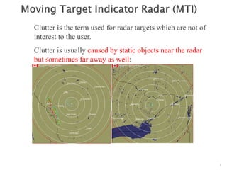
1. 1
n
n
n
n
Clutter is the term used for radar targets which are not of
interest to the user.
Clutter is usually caused by static objects near the radar
but sometimes far away as well:

2. 11/24/2016 2
n
n
n
n
Sometimes clutter can be caused by sidelobes in the
antenna pattern or a poorly adjusted antenna
In any case it is desirable to eliminate as much
clutter as possible

3. 11/24/2016 3
n
n
n
n
This is done by using the fact that the desired target
is usually moving relative to the radar and thus
causes a Doppler shift in the return signal.
The Doppler shift can also be used to determine the
relative speed of the target.

4. 11/24/2016 4
n
n
n
n
The simple CW example can be modified to
incorporate pulse modulation
Note that the same oscillator is used transmission and
demodulation of the return
Thus the return is processed coherently
i.e. the phase of the signal is preserved

5. 11/24/2016 5
n
n
n
n
The transmitted signal is
and the received signal is
these are mixed and the
difference is extracted
This has two components, one is a sine wave at Doppler
frequency, the other is a phase shift which depends on the
range to the target, R0

6. 11/24/2016 6
n
n
n
n
Note that for stationary targets fd = 0 so Vdiff is constant
Depending on the Doppler frequency one two situations will occur
fd>1/τ
fd<1/τ

7. 11/24/2016 7
n
n
n
n
Note that for a pulse width of 1μs, the dividing line is a
Doppler shift of 1 MHz.
If the carrier frequency is 1 GHz, this implies a relative
speed of 30,000 m/s .
Thus all terrestrial radars operate in a sampled mode
and thus are subject to the rules of sampled signals
e.g. Nyquist’s criterion
We shall also see that we can use Discrete Sample
Processing (DSP) to handle some of the problems

8. 11/24/2016 8
n
n
n
n
Looking a successive oscilloscope displays of radar
receiver output we see:
At the ranges of the two
targets, the return amplitude
is varying as the radar
samples the (relatively) slow
Doppler signal.
The bottom trace shows what
would be seen in real time
with the moving targets
indicated by the amplitude
changes.

9. 11/24/2016 9
n
n
n
n
We usually want to process the information
automatically. To do this we take advantage of the fact
that the amplitudes of successive pulse returns are
different:
OR
z-1
-

10. 11/24/2016 10
n
n
n
n
MTI Radar Block Diagrams
MOPA (master oscillator, power amplifier)
Power amplifiers:
Klystron
TWT (Travelling wave tube)
Solid State (Parallel)

11. 11/24/2016 11
n
n
n
n
One of the problems with MTI in pulsed radars is that
magnetrons are ON/OFF devices.
i.e. When the magnetron is pulsed it starts up with a
random phase and is thus its ouput is not coherent with the
pulse before it. Also it can not provide a reference oscillator to
mix with the received signals.
Therefore some means must be provided to maintain the
coherence (at least during a single pulse period)

12. 11/24/2016
ELEC4600 Radar and Navigation
Engineering 12
n
n
n
n
PLL

13. 11/24/2016 13
n
n
n
n
The notes have a section on various types of delay line
cancellers.
This is a bit out of date because almost all radars today
use digitized data and implementing the required
delays is relatively trivial but it also opens up much
more complex processing possibilities.

14. 11/24/2016 14
n
n
n
n
The Filtering Characteristics of a Delay Line Canceller
The output of a single delay canceller is:
This will be zero whenever πfdT is 0 or
a multiple of π
The speeds at which this occurs are
called the blind speeds of the radar
.
where n is
0,1,2,3,…

15. 11/24/2016 15
n
n
n
n
If the first blind speed is to be greater than the highest
expected radial speed the λfp must be large
large λ means larger antennas for a given beamwidth
large fp means that the unambiguous range will be quite small
So there has to be a compromise in the design of an MTI radar

16. 11/24/2016 16
n
n
n
n
The choice of operating with blind speeds or ambiguous
ranges depends on the application
Two ways to mitigate the problem at the expense of increased
complexity are:
a. operating with multiple prfs
b. operating with multiple carrier frequencies

17. 11/24/2016 17
n
n
n
n
Double Cancellation:
Single cancellers do not have a very sharp cutoff at the nulls
which limits their rejection of clutter
(clutter does not have a zero width spectrum)
Adding more cancellers sharpens the nulls

18. 11/24/2016 18
n
n
n
n
Double Cancellation:
There are two implementations:
These have the same frequency response: which is the
square of the single canceller response
)
(
sin
4 2
T
f
v d



19. 11/24/2016 19
n
n
n
n
Double Cancellation:

20. 11/24/2016 20
n
n
n
n
Transversal Filters
These are basically a tapped delay line with the taps
summed at the output

21. 11/24/2016 21
n
n
n
n
Transversal Filters
To obtain a frequency response of sinnπfdT,
the taps must be binomially weighted i.e.

22. 11/24/2016 22
n
n
n
n
Filter Performance Measures
MTI Improvement Factor, IC
in
out
C
C
S
C
S
I
)
/
(
)
/
(

Note that this is averaged over all Doppler frequencies
1/2T
0
Signal Clutter
1/2T
0
Filter

23. 23
n
n
n
n
Filter Performance Measures
Clutter Attenuation ,C/A
The ratio of the clutter power at the input of the canceler
to the clutter power at the output of the canceler
It is normalized, (or adjusted) to the signal attenuation of
the canceler.
i.e. the inherent signal attenuation of the canceler is
ignored

24. 11/24/2016 24
n
n
n
n
Transversal Filters with Binomial Weighting with alternating
sign
Advantages:
Close to optimum for maximizing the Clutter
improvement factor
Also close to maximizing the Clutter Attenuation
Cin/Cout
in
out
C
C
S
C
S
I
)
/
(
)
/
(


25. 11/24/2016 25
n
n
n
n
Transversal Filters with Binomial Weighting with alternating
sign
Disadvantage:
As n increases the sinn filter cuts off more and more of the
spectrum around DC and multiples of PRF
This leads to wider blind speed zones and hence loss of
legitimate targets.