213 221

ISSN: 2278 – 1323
International Journal of Advanced Research in Computer Engineering & Technology
Volume 1, Issue 5, July 2012

Optimized MAC Protocol with Power Efficiency in
Mobile Ad-hoc Network
Rahul Mukherjee
HOD and Assistant Professor, Electronics & Communication Department,
St. Aloysius Institute of Technology (SAIT), Jabalpur, Rajiv Gandhi Technical University, India
rahulmukherjee.sait@gmail.com

Abstract – Mobile Ad-hoc Network (MANET) is an
autonomous system of mobile nodes connected by wireless  Hidden and Exposed Node Issue
links. The nodes are free to move about and organize
themselves into a network. These nodes change position The transmission range of stations in wireless network is
frequently. To accommodate the changing topology special limited by the transmission power; therefore, all the station in
routing algorithms are needed. The Media Access Control a LAN cannot listen to each other. This means that normal
(MAC) data communication protocol sub-layer provides carrier sense mechanism which assumes that all stations can
addressing and channel access control mechanisms that listen to each other, fails. In particular, this gives rise to
make it possible for network nodes to access common hidden node and exposed node problem. Consider stations A,
wireless channel through distributed coordination function B, C and D as shown in figure.
(DCF).This work proposes a new power controlled MAC
protocol based on IEEE 802.11. Network Simulator 2
(NS2) has been used for simulation. It saves considerable
amount of power and achieves the performance matching
with that of IEEE 802.11.
Keywords - MANET, 802.11 MAC, DCF, CSMA

I. INTRODUCTION
A Mobile Ad-hoc network (MANET) is a network formed
and functioning without any established infrastructure or
centralized administration and consists of mobile nodes that
use a wireless interface to communicate with each other.
These mobile nodes serve as both hosts and routers so they
can forward packets on behalf of each other. Hence the
mobile nodes are able to communicate beyond their Figure .2. Hidden & Exposed node problem
transmission range by supporting multihop communication.
Mobile nodes can move freely, and organize themselves
randomly i.e. each host can dynamically enter and leave the
network. Thus, the network topology may change frequently II. CSMA/CA
and rapidly. This means that the network has to adapt itself to
the current topology. A MANET may either work as
The most important part of a MAC protocol is
self-configured stand-alone network or may be connected to
the Internet through gateway nodes. Channel Access Mechanism. The channel access mechanism
is way of regulating the use of physical channel among the
stations present in the network. It specifies when a station can
send or receive data on the channel.

CSMA/CA (Carrier Sense Multiple Access) is derived
from CSMA/CD (Collision Detection) which is the channel
access mechanism used in wired Ethernets. Since the
transmission range of wireless stations is limited, collision
cannot be detected directly. This protocols tries to avoid the
collision. On arrival of a data packet from LLC, a station
senses the channel before transmission and if found idle,
starts transmission. If another transmission is going on, the
station waits for the length of current transmission, and starts
contention. Since the contention is a random time, each
station get statistically equal chance to win the contention.
Figure .1. Ad-hoc Wireless Network

213
All Rights Reserved © 2012 IJARCET

ISSN: 2278 – 1323
III. CLASSIFICATION OF MAC PROTOCOL

MAC protocols for ad-hoc wireless networks can be
classified into several categories based on various criteria
such as initiation approach, time synchronization, and
reservation approach. Ad-hoc Network MAC protocols are
classified in three types;
Contention based protocols.
Contention based protocols with reservation mechanism.
Contention based protocols with scheduling mechanism.

A. Contention Based Protocols
These protocols follow a contention based channel access
policy. A node doesn’t make any resource reservation in
priori. Whenever it receives a packet to be transmitted, it
contends with other nodes for access to the shared channel.
These are further divided into two types;
 Sender initiated protocols
 Receiver initiated protocols
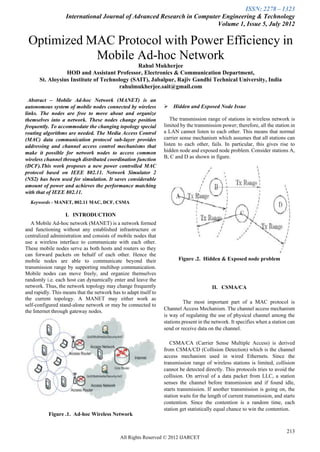
Figure .3. CSMA Channel Access Mechanism
B. Contention Based Protocol with Reservation Mechanisms
CSMA/CA is asynchronous mechanism for medium Ad-hoc wireless networks sometimes may need to support
access and does not provide any bandwidth guarantee. It’s a real time traffic, which requires QoS guarantees to be
best effort service and is suited for packetized applications provided. In order to support such traffic, certain protocols
like TCP/IP. It adapts quite well to the variable traffic have mechanism for reserving bandwidth in priori. These
conditions and is quite robust against interference. protocols are classified into two types;
 Synchronous protocols
 Asynchronous protocols

C. Contention Based Protocol with Scheduling Mechanisms
These protocols focus on packet scheduling at nodes, and
also scheduling nodes for access to the channel. Node
scheduling is done in a manner so that all nodes are treated
fairly. Scheduling based scheme are also used for enforcing
priorities among flows whose packets are queued at nodes.

Figure .4. Flow chart of CSMA/CA Figure .5. MAC Architecture

214

ISSN: 2278 – 1323
IV. IEEE 802.11 OPERATION The IEEE 802.11 MAC is designed for wireless LANs.
The requirements of multi-hop ad-hoc networks are more
The IEEE 802.11 MAC offers two kinds of medium access challenging than those of wireless LANs. In this research, we
methods, namely Distributed Coordination Function (DCF), investigate the operation of IEEE 802.11 MAC in centralized
and Point Coordination Function (PCF). DCF is the basic multi-hop ad-hoc networks. The terms station and node are
access method in 802.11 and requires no infrastructure. used interchangeably throughout the thesis. Multi-hop
cooperative wireless ad-hoc networks will be simply referred
to as multi-hop networks.

Figure .8. Multi-hop Scenario

Consider a multi-hop centralized scenario, as shown in the
figure. For convenience, the stations inside the network are
classified into following categories:
Figure .6. DCF-PCF Coordination Central station : is the central controlling station. Most
of the traffic in the network is directed towards it.
The IEEE 802.11 MAC offers DCF, and PCF. DCF Inner stations : are within one hop boundary of the central
requires no infrastructure. When wireless stations are within station.
transmit range of each other, they form a Basic Service Set
Boundary stations : are at one hop boundary of the
(BSS), and can communicate to each other using DCF. If the
central station. These stations act as relaying stations for the
BSS contains only two stations, it is called Independent Basic
stations outside the reach of central node. Outer stations are
Service Set (IBSS). Many BSSs may be connected by a
outside the communication range of central node.
Distribution System (DS) to form an Extended Service Set
(ESS). An access point (AP) is the station that provides
access to DS services.

Figure .7. 802.11 Architecture

Figure .9. IEEE 802.11 Protocol Architecture

215

ISSN: 2278 – 1323
VI. MAC SUB LAYER IN IEEE 802.11
V. IEEE 802.11 SCHEME SPECIFICATION
The IEEE standard 802.11 specifies the most famous
IEEE 802.11 specifies two medium access control family of WLANs in which many products are already
protocols, PCF (Point Coordination Function) and DCF available. This means that the standard specifies the physical
(Distributed Coordination Function). PCF is a centralized and medium access layer adapted to the special requirements
scheme, whereas DCF is a fully distributed scheme. We of wireless LANs, but offers the same interface as the others
consider DCF in this paper. to higher layers to maintain interoperability.

 SYSTEM ARCHITECTURE
 Transmission range : When a node is within transmission
range of a sender node, it can receive and correctly decode The basic service set (BSS) is the fundamental building
packets from the sender node. In our simulations, the block of the IEEE 802.11 architecture. A BSS is defined as a
transmission range is 250 m when using the highest group of stations that are under the direct control of a single
transmit power level. coordination function (i.e., a DCF or PCF) which is defined
below. The geographical area covered by the BSS is known
 Carrier sensing range : Nodes in the carrier sensing as the basic service area (BSA), which is analogous to a cell
range can sense the sender’s transmission. Carrier sensing in a cellular communications network.
range is typically larger than the transmission range, for
instance, two times larger than the transmission range. In Conceptually, all stations in a BSS can communicate
our simulations, the carrier sensing range is 550 m when directly with all other stations in a BSS. However,
using the highest power level. Note that the carrier transmission medium degradations due to multipath fading,
sensing range and transmission range depend on the or interference from nearby BSSs reusing the same
transmit power level. physical-layer characteristics (e.g., frequency and spreading
code, or hopping pattern), can cause some stations to appear
hidden from other stations. An ad hoc network is a deliberate
 Carrier sensing zone : When a node is within the carrier
grouping of stations into a single BSS for the purposes of
sensing zone, it can sense the signal but cannot decode it internetworked communications without the aid of an
correctly. Note that, as per our definition here, the carrier infrastructure network. Given figure is an illustration of an
sensing zone does not include transmission range. Nodes independent BSS (IBSS), which is the formal name of an ad
in the transmission range can indeed sense the hoc network in the IEEE 802.11 standard. Any station can
transmission, but they can also decode it correctly. establish a direct communications session with any other
Therefore, these nodes will not be in the carrier sensing station in the BSS, without the requirement of channeling all
zone as per our definition. The carrier sensing zone is traffic through a centralized access point (AP).
between 250 m and 550 m with the highest power level in
our simulation.

Figure .11. System Architecture of an Ad-hoc network

In contrast to the ad hoc network, infrastructure networks
are established to provide wireless users with specific
services and range extension. Infrastructure networks in the
Figure .10. Carrier Sensing context of IEEE 802.11 are established using APs. The AP
supports range extension by providing the integration points
necessary for network connectivity between multiple BSSs,
thus forming an extended service set (ESS). The ESS has the
appearance of one large BSS to the logical link control (LLC)
sub layer of each station (STA). The ESS consists of multiple

216

ISSN: 2278 – 1323
BSSs that are integrated together using a common A. Inter frame Spacing
distribution system (DS). The DS can be thought of as a IFS is the time interval between frames. IEEE 802.11
backbone network that is responsible for MAC-level defines four IFSs – SIFS (short inter frame space), PIFS (PCF
transport of MAC service data units (MSDUs). inter frame space), DIFS (DCF inter frame space), and EIFS
(extended inter frame space). The IFSs provide priority levels
for accessing the channel. The SIFS is the shortest of the inter
frame spaces and is used after RTS, CTS, and DATA frames
to give the highest priority to CTS, DATA and ACK,
respectively. In DCF, when the channel is idle, a node waits
for the DIFS duration before transmitting any packet.

In figure, nodes in transmission range correctly set their
NAVs when receiving RTS or CTS. However, since nodes in
the carrier sensing zone cannot decode the packet, they do not
know the duration of the packet transmission. To prevent a
collision with the ACK reception at the source node, when
nodes detect a transmission and cannot decode it, they set
their NAVs for the EIFS duration. The main purpose of the
EIFS is to provide enough time for a source node to receive
Figure .12. Example of infrastructure network the ACK frame, so the duration of EIFS is longer than that of
an ACK transmission. As per IEEE 802.11, the EIFS is
VII. DCF OPERATION obtained using the SIFS, the DIFS, and the length of time to
transmit an ACK frame at the physical layer’s lowest
The DCF is the fundamental access method used to mandatory rate, as the following equation :
support asynchronous data transfer on a best effort basis. The
DCF is based on CSMA/CA. The carrier sense is performed
at both the air interface, referred to as physical carrier EIFS = SIFS + DIFS + [(8·ACKsize) + Preamble
sensing, and at the MAC sub layer, referred to as virtual Length + PLCP Header Length] / Bit Rate
carrier sensing. Physical carrier sensing detects presence of
other users by analyzing the activity in the channel through where ACK size is the length (in bytes) of an ACK frame, and
the received signal strength. Bit Rate is the physical layer’s lowest mandatory rate. Preamble
A station performs virtual carrier sense by Length is 144 bits and PLCP Header Length is 48 bits . Using a 1
examining the received MPDU (MAC Protocol Data Unit) Mbps channel bit rate, EIFS is equal to 364 μs.
information in the header of RTS, CTS and ACK frames. The
stations in BSS use this information to adjust their Network
Allocation Vector (NAV), which indicates amount of time
that must elapse until the current transmission is complete
and the channel can be sampled again for idle status.

Figure .14. NAV duration in transmission range and
carrier sensing zone

VIII. BASIC POWER CONTROL PROTOCOL

Here nodes A and B send RTS and CTS, respectively, with
the highest power level so that node C receives the CTS and
defers its transmission. By using a lower power for DATA
Figure .13. DCF access using RTS/CTS and ACK packets, nodes can conserve energy.

217

ISSN: 2278 – 1323

Figure .15. Basic Scheme.

In the Basic scheme, the RTS–CTS handshake is used to
decide the transmission power for subsequent DATA and
ACK packets. This can be done in two different ways as
Figure .16. Basic Power Control Protocol.
described below. Let pmax denote the maximum possible
transmit power level.
IX. DEFICIENCY OF THE BASIC PROTOCOL
 Suppose that node A wants to send a packet to node B.
In the Basic scheme, RTS and CTS are sent using
Node A transmits the RTS at power level pmax. When
pmax, and DATA and ACK packets are sent using the
B receives the RTS from A with signal level pr, B can
minimum necessary power to reach the destination. When the
calculate the minimum necessary transmission power
neighbour nodes receive an RTS or CTS, they set their NAVs
level, pdesired, for the DATA packet based on received
for the duration of the DATA–ACK transmission. When D
power level pr, the transmitted power level, pmax, and
and E transmit the RTS and CTS, respectively, B and C
noise level at the receiver B.
receive the RTS, and F and G receive the CTS, so these nodes
We can borrow the procedure for estimating pdesired will defer their transmissions for the duration of the D–E
from. This procedure determines pdesired taking into account transmission. Node A is in the carrier sensing zone of D
the current noise level at node B. Node B then specifies (when D transmits at pmax) so it will only sense the signals
pdesired in its CTS to node A. After receiving CTS, node A and cannot decode the packets correctly. Node A will set its
sends DATA using power level pdesired. Since the NAV for EIFS duration when it senses the RTS transmission
signal-to-noise ratio at the receiver B is taken into from D. Similarly, node H will set its NAV for EIFS duration
consideration, this method can be accurate in estimating the following CTS transmission from E.
appropriate transmit power level for DATA. When transmit power control is not used, the carrier
sensing zone is the same for RTS–CTS and DATA–ACK
 In the second alternative, when a destination node
since all packets are sent using the same power level.
However, in Basic, when a source and destination pair
receives an RTS, it responds by sending a CTS as usual
decides to reduce the transmit power for DATA–ACK, the
(at power level p max). When the source node receives
transmission range for DATA–ACK is smaller than that of
the CTS, it calculates p desired based on received
RTS–CTS; similarly, the carrier sensing zone for
power level, pr, and transmitted power level (p max), as
DATA–ACK is also smaller than that of RTS–CTS.

P desired = p max/pr · Rxthresh · c,

where Rxthresh is the minimum necessary received signal
strength and c is a constant. We set c equal to 1 in our
simulations. Then, the source transmits DATA using a power
level equal to p desired. Similarly, the transmit power for the
ACK transmission is determined when the destination
receives the RTS.

Figure .17. Basic Scheme

218

ISSN: 2278 – 1323
X. PROPOSED POWER CONTROL MAC PROTOCOL transmissions at pmax is 210 μs, which is shorter than EIFS
duration. A source node starts transmitting DATA at pmax
Proposed power control MAC (PCM) is similar to the for 20 μs and reduces the transmit power to a power level
Basic scheme in that it uses power level pmax for RTS–CTS adequate for the given transmission for 190 μs. Then, it
and the minimum necessary transmit power for DATA–ACK repeats this process during DATA transmission. The node
transmissions. We now describe the procedure used in PCM. also transmits DATA at pmax for the last 20 μs of the
transmission.
1. Source and destination nodes transmit the RTS and CTS
With the above simple modification, PCM
using pmax. Nodes in the carrier sensing zone set their NAVs
overcomes the problem of the BASIC scheme and can
for EIFS duration when they sense the signal and cannot
achieve efficiency comparable to 802.11, but uses less
decode it correctly.
energy.
2. The source node may transmit DATA using a lower
The proposed power control protocol is modified such that
power level, similar to the BASIC scheme.
in this the Data and ACK is transmitted at lower power level
3. To avoid a potential collision with the ACK (as but after a certain duration it is transmitted at higher power
discussed earlier), the source node transmits DATA at the level for a very fraction of time, in order to make the
power level pmax, periodically, for just enough time so that neighboring nodes understand that transmission is going on
nodes in the carrier sensing zone can sense it. and they should restrict their transmission during that period
so that collision does not take place hence saving power
4. The destination node transmits an ACK using the consumption.
minimum required power to reach the source node, similar to
the BASIC scheme.
Figure shows how the transmit power level changes
during the sequence of an RTS–CTS–DATA–ACK
transmission. After the RTS–CTS handshake using pmax,
suppose the source and destination nodes decide to use power
level p1 for DATA and ACK. Then, the source will transmit
DATA using p1 and periodically use pmax. The destination
uses p1 for ACK transmission.

Figure .18. PCM periodically increases

The main difference between PCM and the Basic scheme
is that PCM periodically increases the transmit power to
pmax during the DATA packet transmission. With this
change, nodes that can potentially interfere with the reception
of ACK at the sender will periodically sense the channel as
busy, and defer their own transmission.
Accordingly, 15 μs should be adequate for carrier
sensing, and time required to increase output power (power
on) from 10% to 90% of maximum power (or power-down
from 90% to 10% of maximum power) should be less than 2
μs. Thus, we believe 20 μs should be enough to power up (2
μs), sense the signal (15 μs), and power down (2 μs). In our
simulation, EIFS duration is set to 212 μs using a 2 Mbps Figure .19. Flow chart of Proposed Protocol
bit rate. In PCM, a node transmits DATA at pmax every 190
μs for a 20μs duration. Thus, the interval between the
219

ISSN: 2278 – 1323
XI. SIMULATION RESULTS
The given table shows all the different parameters taken
into account for conducting the simulation in NS-2
atmosphere. In this table the values of all the different
parameters are shown, using which the simulation for
aggregate throughput and total data delivered per joule in
accordance with Data rate per flow and Packet size is
calculated for all three schemes namely, BASIC, 802.11 and
Proposed protocol’s.

Parameters Values
Number of nodes 50
Simulation Area(m) 800x800
Topology Random
Transmission range 50,100,150,200,250
C. Simulation Result for Data Delivered per Joule vs Data
Radio Propagation model Shadowing
rate per flow
Traffic model CBR, TCP
Packet Size 256,512,1024 bytes
Simulation times 150 seconds,300 seconds
Bandwidth 2 Mbps
Routing DSR

A. Simulation Result for Aggregate Throughput vs Data
Rate Per Flow

D. Simulation Result for Data Delivered per joule vs
Packet Size

B. Simulation Result for Aggregate Throughput vs Packet
Size

220

ISSN: 2278 – 1323
XII. CONCLUSION [6] Performance analysis of AODV,DSDV AND DSR in
MANETS, International Journal of Distributed and
It is shown that the Basic scheme increases collisions and Parallel Systems (IJDPS) Vol.2, No.6, November 2011
retransmissions, which can result in more energy
consumption and throughput degradation. Hence, the [7] Geetha jayakumar and G Gopinath – ―Performance
proposed protocol is more efficient than Basic scheme and comparison of Two On- demand routing protocols for
802.11 yielding better throughput Ad-hoc Networks based on random way point mobility
model.‖ – Department of Computer Science,
Bharathidasan University, Triuchirapalli- 620 023,
India

XIII. SUGGESTION FOR FUTURE WORK

 We have shown the throughput of proposed protocol
comparable to 802.11 with less power consumption for
random topology ad hoc network.
 In future the same power consumption scheme will be
conducted for grid topology.

One possible approach to the mobile ad hoc network
power control scheme is that, it is only applied to the Random Rahul Mukherjee : H.O.D. & Asst Prof. (EC-Deptt),
topology ad hoc scenario but it can also be made applicable St. Aloysius Institute of Technology (SAIT), Jabalpur, India.
for Grid Topology power control scheme without degrading Pursuing P.hd in the field of Mobile Ad-hoc Network.
the network throughput. Where the nodes will be placed Published research papers in five international journals.
sequentially in a proper manner i.e, in an arranged fashion. Completed B.E.(EC) from RGPV, Bhopal. Pursued M.Tech
in Communication Systems Engineering from KIIT
University, Bhubaneswar. His field of interests comprises of
Mobile Technology & Wireless Networking.
XIV. REFERENCES

[1] B. Awerbunch,D. Holmer, and H. Rubens .The medium
time metric: High throughput route selection in
multi-rate adhoc wireless network.

[2] Ruay-Shiung Chang and Shing-Jiuan Leu, January
2006,”Long-lived Path Routing With Received Signal
Strength for Ad Hoc Networks”, IEEE International
Symposium on Wireless Pervasive Computing.

[3] R. Wattenhofer, L. Li, P. Bahl and Y.-M. Wang,
Distributed topology control for power efficient
operation in multihop wireless ad hoc networks,Vol. 3
pp. 1388–1397 (April 2001).

[4] N. Poojary, S.V. Krishnamurthy and S. Dao, Medium
access control in a network of ad hoc mobile nodes with
heterogeneous power capabilities, in: Proc. IEEE
International Conference on Communications (ICC
2001), Vol. 3 pp. 872–877 (2001).

[5] M.K.Marina and S.R.Das, 2001, “On-Demand
Multipath distance vector routing in ad hoc Networks”
in: Proceedings of 9th IEEE International Conference
on Network Protocols (ICNP).

221

213 221

Recommended

Recommended

More Related Content

What's hot

What's hot (19)

Viewers also liked

Viewers also liked (9)

Similar to 213 221

Similar to 213 221 (20)

More from Editor IJARCET

More from Editor IJARCET (20)

Recently uploaded

Recently uploaded (20)

213 221