Hadoop sensordata part2
•
1 recomendación•839 vistas

Terabyte scale Sensor Network data analysis using MapReduce/ Hadoop

Recomendados
Más contenido relacionado
La actualidad más candente
La actualidad más candente (17)
Destacado
Similar a Hadoop sensordata part2
Similar a Hadoop sensordata part2 (20)
Más de Joaquin Vanschoren
Más de Joaquin Vanschoren (19)
Último
Último (20)
Hadoop sensordata part2
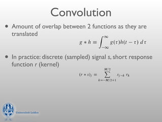
- 1. 2 if0 t h.t / e ” H.f f / frequency shiftin Figure 13.1.2. Convolution of discretely sampled functions. Note how the response function fo 0 Convolution times is wrapped around and stored at the extreme right end of the array rk . With two functions h.t / and g.t /, and their corresponding H.f / and G.f /, we can form two combinations of special intere • Amount of Example: Abetween g functions 1asbyall other rk ’s equal of the two functions, denoted 2 h, is r0 D and overlap response function with defined they are translatedjust the identity filter. Convolution Zis1signal with this response functio is of a identically the signal. Another example the response function with r14 D hÁ all other rk ’s equal to zero.gThis produces convolved output / d is the inpu g. /h.t that 1 multiplied by 1:5 and delayed by 14 sample intervals. • In Evidently, we have just described in words the following definition of practice: discrete a(sampled) theof finitedomain M : that g h D Note convolution witha function in signal s,duration and that g h is response function time short response that the function g h is one member of a simple transform pair, function r (kernel) M=2 X g h ” G.f /H.f / .r s/j Á convolution theorem sj k rk kD M=2C1 In other words, the Fourier transform of the convolution is just individual Fourier transforms.is nonzero only in some range M=2 < k Ä If a discrete response function The correlation of two functions, denoted Corr.g; h/, is defi where M is a sufficiently large even integer, then the response function is finite impulse response (FIR), and its duration is M . (Notice that we are defi Z 1 as the number of nonzero values of rk ; these values span a time interval of Corr.g; circumstances the C t /h. / d is the sampling times.) In most practicalh/ Á g. case of finite M interest, either because the response really has1finite duration, or because we a
- 2. 2 if0 t h.t / e ” H.f f / frequency shiftin Figure 13.1.2. Convolution of discretely sampled functions. Note how the response function fo 0 Convolution times is wrapped around and stored at the extreme right end of the array rk . With two functions h.t / and g.t /, and their corresponding H.f / and G.f /, we can form two combinations of special intere • Amount of Example: Abetween g functions 1asbyall other rk ’s equal of the two functions, denoted 2 h, is r0 D and overlap response function with defined they are translatedjust the identity filter. Convolution Zis1signal with this response functio is of a identically the signal. Another example the response function with r14 D hÁ all other rk ’s equal to zero.gThis produces convolved output / d is the inpu g. /h.t that 1 multiplied by 1:5 and delayed by 14 sample intervals. • In Evidently, we have just described in words the following definition of practice: discrete a(sampled) theof finitedomain M : that g h D Note convolution witha function in signal s,duration and that g h is response function time short response that the function g h is one member of a simple transform pair, function r (kernel) M=2 X g h ” G.f /H.f / .r s/j Á convolution theorem sj k rk kD M=2C1 In other words, the Fourier transform of the convolution is just individual Fourier transforms. convolution If a discrete response function is nonzero only in some range M=2 < k Ä The correlation of two functions, denoted Corr.g; h/, is defi where M is a sufficiently large even integer, then the response function is signal finite impulse response (FIR), and its duration is M . (Notice that we are defi Z 1 as the number of nonzero values of rk ; these values span a time interval of Corr.g; circumstances the C t /h. / d is the sampling times.) In most practicalh/ Á g. case of finite M kernel interest, either because the response really has1finite duration, or because we a
- 3. Convolution • Width of kernel defines smoothing strength
- 4. Convolution • Width of kernel defines smoothing strength convolution 1 convolution 2 signal kernel 1 kernel 2
- 5. Convolution • Width of kernel defines smoothing strength convolution 1 convolution 2 signal kernel 1 kernel 2 • Quite fast (O(N*M)), not fast enough
- 6. Convolution • Width of kernel defines smoothing strength convolution 1 convolution 2 signal kernel 1 kernel 2 • Quite fast (O(N*M)), not fast enough
- 7. Map Reduce
- 8. Map Reduce
- 9. Map Map Map Map Map Reduce
- 10. Map Map Map Map Map Reduce Reduce Reduce Reduce Reduce
- 11. Map Map Map Map Map Reduce Reduce Reduce Reduce Reduce
- 12. Build Build Build Build Build Map Map Map Map Map windows windows windows windows windows Reduce Reduce Reduce Reduce Reduce
- 13. Build Build Build Build Build Map Map Map Map Map windows windows windows windows windows Reduce Reduce Reduce Reduce Reduce
- 14. Build Build Build Build Build Map Map Map Map Map windows windows windows windows windows Shuffle Reduce Reduce Reduce Reduce Reduce
- 15. Build Build Build Build Build Map Map Map Map Map windows windows windows windows windows Shuffle Reduce Convolute Reduce Convolute Reduce Convolute Reduce Convolute Reduce Convolute
- 16. Build Build Build Build Build Map Map Map Map Map windows windows windows windows windows Shuffle Reduce Convolute Reduce Convolute Reduce Convolute Reduce Convolute Reduce Convolute
- 17. Build Build Build Build Build Map Map Map Map Map windows windows windows windows windows Shuffle Reduce Convolute Reduce Convolute Reduce Convolute Reduce Convolute Reduce Convolute
- 18. i Convolution in Hadoop “nr3” — 2007/5/1 — 20:53 — page 644 — #666 644 • Wrap-around problem Chapter 13. Fourier and Spectral Applications response function m+ m− sample of original function m+ m− convolution spoiled unspoiled spoiled
- 19. Convolution in Hadoop spoiled convolution unspoiled spoiled • Wrap-around problem Figure 13.1.3. The wraparound problem in convolving finite segments of a function. Not only must the response function wrap be viewed as cyclic, but so must the sampled original function. Therefore, a portion at each end of the original function is erroneously wrapped around by convolution with the • Ignore spoiled regions response function. response function • Mirror the sequence (works well in our case) m+ m− • Zero-padding original function zero padding m− m+ not spoiled because zero m+ m− unspoiled spoiled but irrelevant
- 20. Convolution in Hadoop • Data split problem: windowing • `Overlap-convolute’
- 21. Convolution in Hadoop • Data split problem: windowing • `Overlap-convolute’ Map (window) timestamp1 timestamp2 timestamp3
- 22. Convolution in Hadoop • Data split problem: windowing • `Overlap-convolute’ Mapper1 Mapper2 Mapper3 Map (window) 1 2 1 2 3 2 3 timestamp1 timestamp2 timestamp3
- 23. Convolution in Hadoop • Data split problem: windowing • `Overlap-convolute’ Mapper1 Mapper2 Mapper3 Map (window) 1 2 1 2 3 2 3 timestamp1 timestamp2 Reduce (convolute) timestamp3
- 24. Convolution in Hadoop • Data split problem: windowing • `Overlap-convolute’ Mapper1 Mapper2 Mapper3 Map (window) 1 2 1 2 3 2 3 timestamp1 timestamp2 Reduce (convolute) timestamp3 Emit only unpolluted data
- 25. Convolution in Hadoop • Data split problem: windowing • `Convolute-add’
- 26. Convolution in Hadoop • Data split problem: windowing • `Convolute-add’ Map 0 0 (convolute 0 0 with 0-padding) 0 0
- 27. Convolution in Hadoop • Data split problem: windowing • `Convolute-add’ Map (convolute with 0-padding) Reduce (add) A A+B B B+C C Add values in overlapping regions
- 28. Hint: Keep mappers alive • Mappers will be killed if you spend too much time in a loop (e.g. during long convolutions) • Do this in large loops: • for(loopcount%1000==0){context.progress();}
- 29. Even faster: Fourier Transform • Converts signal from time domain to frequency domain • Stress sensor (time domain) •f • Fourier transform (frequency domain)
- 30. Discrete Fourier Transform • Converts signal from time domain to frequency domain • Vibration sensor (time domain) • Fourier transform (frequency domain)
- 31. H.f / and G.f /, we can form two combinatio of the two functions, denoted g h, is defined DFT for convolution g hÁ Z 1 g. /h • Convolution theorem: Note that gtransform of convolution i Fourier h is a function in the time domai 1 is product of individualthat the 2007/5/1 — 20:53 one page 643 of a#665 Fourier transforms— member — sim i “nr3” — function g h is g h ” G.f /H.f / conv • Discrete convolution13.1 Convolution and the Fourier transform FFTthe c theorem: In other words, Deconvolution Using the of individual Fourier transforms. The correlation of two functions, denoted N=2 X sj k rk ” Sn Rn Z 1 • Conditions: kD N=2C1 Corr.g; h/ Á g. 1 • Signal periodic: 0-padding (see above) of t , which is call Here Sn .n D 0; : : : ; N 1/ is the discrete Fourier transform of the valu The correlation is a function 0; : : : ; N 1/, while Rn .n D 0; : : : ; N 1/ is the discrete Fourier t • Signals of same length: Pad response ” G.f /H .f /0s c domain, and it turns out to be one member of t the values rk .k D 0; : : : ; N 1/. These values of rk are the same as f function with k D N=2 C 1; : : : ; N=2, but in wraparound order, exactly as was desc end of 12.2. Corr.g; h/ 13.1.1 Treatment of End Effects by Zero Paddingpai [More generally, the second member of the
- 32. Discrete Fourier Transform • DFT is O(NlogN) • In Hadoop: • Modification of Parallel-FFT • Convolution: • MR-DFT • Take product of both FTs • inverse MR-DFT
- 33. Segmentation Windowing Windowing Windowing Windowing Windowing Shuffle Convolute Convolute Convolute Convolute Convolute G’,G’’,G’’’ G’,G’’,G’’’ G’,G’’,G’’’ G’,G’’,G’’’ G’,G’’,G’’’ Emit zero-crossings
- 34. Segmentation signal convolution segmentation 1st, 2nd,3rd degree derivatives