FUll download : https://alibabadownload.com/product/econometric-analysis-8th-edition-greene-solutions-manual/ Econometric Analysis 8th Edition Greene Solutions Manual

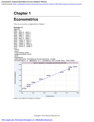
1. Copyright © 2018 Pearson Education, Inc.
Chapter 1
Econometrics
There are no exercises or applications in Chapter 1.
Example 1.2
import$
Year, X,C
2000, 8559.4, 6830.4
2001, 8883.3, 7148.8
2002, 9060.1, 7439.2
2003, 9378.1, 7804.0
2004, 9937.2, 8285.1
2005, 10485.9, 8819.0
2006, 11268.1, 9322.7
2007, 11894.1, 9826.4
2008, 12238.8, 10129.9
2009, 12030.3, 10088.5
plot
;lhs=x
;rhs=c
;limits=6500,10500
;endpoints=8500,12500
;grid
;regression
;vaxis=Personal Consumption;Footer=Personal Income
;Title=Figure 1.1 Aggregate U.S. Consumption and Income Data, 2000-2009$
(Dates were added to the figure by editing.)
Econometric Analysis 8th Edition Greene Solutions Manual
Full Download: https://alibabadownload.com/product/econometric-analysis-8th-edition-greene-solutions-manual/
This sample only, Download all chapters at: AlibabaDownload.com

2. 2
Chapter 2
The Linear Regression Model
There are no exercises or applications in Chapter 2.
Example 2.1. Keynes’s Consumption
import$
Year X C W
1940 241 226 0
1941 280 240 0
1942 319 235 1
1943 331 245 1
1944 345 255 1
1945 340 265 1
1946 332 295 0
1947 320 300 0
1948 339 305 0
1949 338 315 0
1950 371 325 0
plot;lhs=x;rhs=c;limits=200,350; endpoints=225,375;regression
;title=Figure 2.1 Consumption Data, 1940-1950 $
(Dates and dashed lines were added by editing.)

3. 3
Example 2.7. Nonzero Conditional Mean of the Disturbances

4. 4
Chapter 3
Least Squares Regression
EXAMPLES – Section 3.2.2 and Table 3.2
Import$
YEAR RealGNP Invest GNPDefl Interest Infl Trend RealInv
2000 87.1 2.034 81.9 9.23 3.4 1 2.484
2001 88.0 1.929 83.8 6.91 1.6 2 2.311
2002 89.5 1.925 85.0 4.67 2.4 3 2.265
2003 92.0 2.028 86.7 4.12 1.9 4 2.339
2004 95.5 2.277 89.1 4.34 3.3 5 2.556
2005 98.7 2.527 91.9 6.19 3.4 6 2.750
2006 101.4 2.681 94.8 7.96 2.5 7 2.828
2007 103.2 2.644 97.3 8.05 4.1 8 2.717
2008 102.9 2.425 99.2 5.09 0.1 9 2.445
2009 100.0 1.878 100.0 3.25 2.7 10 1.878
2010 102.5 2.101 101.2 3.25 1.5 11 2.076
2011 104.2 2.240 103.3 3.25 3.0 12 2.168
2012 105.6 2.479 105.2 3.25 1.7 13 2.356
2013 109.0 2.648 106.7 3.25 1.5 14 2.482
2014 111.6 2.856 108.3 3.25 0.8 15 2.637
EndData
Create ; Y = RealInv $
Create ; T = trend $
Create ; G = realgnp $
Create ; R = interest $
Create ; P = infl $
Namelist;z=y,t,g,r,p$
Dstat ; rhs=z$
--------+---------------------------------------------------------------------
| Standard Missing
Variable| Mean Deviation Minimum Maximum Cases Values
--------+---------------------------------------------------------------------
Y| 2.420067 .262666 1.878 2.828 15 0
T| 8.0 4.472136 1.0 15.0 15 0
G| 99.41333 7.525468 87.1 111.6 15 0
R| 5.070667 2.081351 3.25 9.23 15 0
P| 2.26 1.092703 .1 4.1 15 0
--------+---------------------------------------------------------------------
Descriptive Statistics for 5 variables
Dstat results are matrix LASTDSTA in current project.
Regress;Lhs=y;rhs=one,t,g,r,p$
-----------------------------------------------------------------------------
Ordinary least squares regression ............
LHS=Y Mean = 2.42007
Standard deviation = .26267
---------- No. of observations = 15 DegFreedom Mean square
Regression Sum of Squares = .760908 4 .19023
Residual Sum of Squares = .205002 10 .02050
Total Sum of Squares = .965911 14 .06899
---------- Standard error of e = .14318 Root MSE .11691
Fit R-squared = .78776 R-bar squared .70287
Model test F[ 4, 10] = 9.27926 Prob F > F* .00213
--------+--------------------------------------------------------------------
| Standard Prob. 95% Confidence
Y| Coefficient Error t |t|>T* Interval
--------+--------------------------------------------------------------------
Constant| -6.26176*** 1.93671 -3.23 .0090 -10.57700 -1.94651

5. 5
T| -.16187*** .04739 -3.42 .0066 -.26746 -.05628
G| .09960*** .02421 4.11 .0021 .04566 .15355
R| .01972 .03380 .58 .5725 -.05559 .09503
P| -.01109 .03990 -.28 .7867 -.09998 .07781
--------+--------------------------------------------------------------------
***, **, * ==> Significance at 1%, 5%, 10% level.
Model was estimated on Aug 01, 2017 at 08:37:09 AM
-----------------------------------------------------------------------------
Namelist; x=one,t,g,r,p$
Matrix ; list;x'x$
--------+----------------------------------------------------------------------
RESULT| 1 2 3 4 5
--------+----------------------------------------------------------------------
1| 15.0000 120.000 1491.20 76.0600 33.9000
2| 120.000 1240.00 12381.5 522.060 244.100
3| 1491.20 12381.5 149038. 7453.03 3332.83
4| 76.0600 522.060 7453.03 446.323 186.656
5| 33.9000 244.100 3332.83 186.656 93.3300
Matrix ; list;x'y$
--------+--------------
RESULT| 1
--------+--------------
1| 36.3010
2| 288.691
3| 3612.90
4| 188.300
5| 82.8193
Matrix ; list;<x'x>*x'y$
--------+--------------
RESULT| 1
--------+--------------
1| -6.26176
2| -.161870
3| .0996027
4| .0197220
5| -.0110883
Matrix ; list;xcor(z)$
--------+--------------------------------------------
Cor.Mat.| Y T G R P
--------+--------------------------------------------
Y| 1.00000 -.10441 .14809 .55261 .19388
T| -.10441 1.00000 .95910 -.66317 -.39612
G| .14809 .95910 1.00000 -.49410 -.32384
R| .55261 -.66317 -.49410 1.00000 .46358
P| .19388 -.39612 -.32384 .46358 1.00000
Create ; dy = dev(y) $
Create ; dt = dev(t) $
Create ; dg = dev(g) $
Calc ; list ; xbr(y)
; xbr(t)
; xbr(g) $
[CALC] = 2.4200667
[CALC] = 8.0000000
[CALC] = 99.4133333
Calculator: Computed 3 scalar results
Calc ; list ; sty = dt'dy
; sgg = dg'dg
; sgy = dg'dy
; stg = dt'dg
; stt = dt'dt$
[CALC] STY = -1.7170000
[CALC] SGG = 792.8573333

6. 6
[CALC] SGY = 4.0982867
[CALC] STG = 451.9000000
[CALC] STT = 280.0000000
Calculator: Computed 5 scalar results
Calc ; list ; b2 = (sty*sgg - sgy*stg)/(stt*sgg-stg*stg)$
[CALC] B2 = -.1806630
Calc ; list ; b3 = (sgy*stt - sty*stg)/(stt*sgg-stg*stg)$
[CALC] B3 = .1081404
Calc ; list ; b1 = xbr(y) - b2*xbr(t)-b3*xbr(g)$
[CALC] B1 = -6.8852242
Calc ; list ; byg = sgy / sgg $
[CALC] BYG = .0051690
Calc ; list ; byt = sty / stt $
[CALC] BYT = -.0061321
Calc ; list ; btg = stg / sgg$
[CALC] BTG = .5699638
Calc ; list ; r2gt=stg^2/(sgg*stt)$
[CALC] R2GT = .9198809
Calc ; list ; byg_t=byg-((byt*btg-r2gt*byg)/(1-r2gt))$
[CALC] BYG_T = .1081404
Namelist ; yvar=y $
Matrix;list;xcor(x,yvar)$
--------+--------
Cor.Mat.| Y
--------+--------
ONE| .00000
T| -.10441
G| .14809
R| .55261
P| .19388
Regress;quietly ; Lhs=y;rhs=one,t,g,r,p$
Matrix ; vars = diag(varb) ; sdevs=sqrt(vars)$
Matrix ; tstats = <sdevs>*b$
Matrix ; pcor = dirp(tstats,tstats) + degfrdm$
Matrix ; pci = diri(pcor)$
Matrix ; pcor = dirp(tstats,tstats,pci)$
Matrix ; list ; pcor = esqr(pcor)$
--------+--------------
PCOR| 1
--------+--------------
1| .000000
2| .733814
3| .792847
4| .181449
5| .0875491

7. 7
Exercises
1. Let
11
... ...
1 n
x
x
 
 
 
 
X .
(a) The normal equations are given by (3-12), X'e 0 (we drop the minus sign), hence for each of the columns
of X, xk, we know that xke = 0. This implies that 1 0n
i ie  and 1 0n
i i ix e  .
(b) Use 1
n
i ie to conclude from the first normal equation that a y bx  .
(c) We know that 1 0n
i ie  and 1 0n
i i ix e  . It follows then that 1( ) 0n
i i ix x e   because
1 1 0n n
i i i ixe x e     . Substitute ei to obtain 1( )( ) 0n
i i i ix x y a bx    
or 1( )( ( )) 0n
i i i ix x y y b x x     
Then, 1
1 1 2
1
( )( )
( )( ) ( )( )) so .
( )
n
n n i i i
i i i i i i n
i i
x x y y
x x y y b x x x x b
x x

 

  
       
 
(d) The first derivative vector of ee is -2Xe. (The normal equations.) The second derivative matrix is
2
(ee)/bb = 2XX. We need to show that this matrix is positive definite. The diagonal elements are 2n
and 2
12 n
i ix which are clearly both positive. The determinant is
[(2n)( 2
12 n
i ix )] - ( 12 n
i ix )2
= 2
14 n
i in x -4( nx )2
= 2 2 2
1 14 [( ) ] 4 [( ( ) ]n n
i i i in x nx n x x      .
Note that a much simpler proof appears after (3-6).
2. Write c as b + (c - b). Then, the sum of squared residuals based on c is
(y - Xc)(y - Xc) = [y - X(b + (c - b))] [y - X(b + (c - b))] = [(y - Xb) + X(c - b)] [(y - Xb) + X(c - b)]
= (y - Xb) (y - Xb) + (c - b) XX(c - b) + 2(c - b) X(y - Xb).
But, the third term is zero, as 2(c - b) X(y - Xb) = 2(c - b)Xe = 0. Therefore,
(y - Xc) (y - Xc) = ee + (c - b) XX(c - b)
or (y - Xc) (y - Xc) - ee = (c - b) XX(c - b).
The right hand side can be written as dd where d = X(c - b), so it is necessarily positive. This confirms what
we knew at the outset, least squares is least squares.
3. In the regression of y on i and X, the coefficients on X are b = (XM0
X)-1
XM0
y. M0
= I - i(ii)-1
i is the
matrix which transforms observations into deviations from their column means. Since M0
is idempotent and
symmetric we may also write the preceding as [(XM0
)(M0
X)]-1
(XM0
)(M0
y) which implies that the regression
of M0
y on M0
X produces the least squares slopes. If only X is transformed to deviations, we would compute
[(XM0
)(M0
X)]-1
(XM0
)y but, of course, this is identical. However, if only y is transformed, the result is
(XX)-1
XM0
y which is likely to be quite different.
4. What is the result of the matrix product M1M where M1 is defined in (3-19) and M is defined in (3-14)?
M1M = (I - X1(X1X1)-1
X1)(I - X(XX)-1
X) = M - X1(X1X1)-1
X1M
There is no need to multiply out the second term. Each column of MX1 is the vector of residuals in the regression
of the corresponding column of X1 on all of the columns in X. Since that x is one of the columns in X, this
regression provides a perfect fit, so the residuals are zero. Thus, MX1 is a matrix of zeroes which implies that
M1M = M.
5. The original X matrix has n rows. We add an additional row, xs. The new y vector likewise has an additional
element. Thus, , ,and .n n
n s n s
s sy
   
       
X y
X y
x
The new coefficient vector is
bn,s = (Xn,s Xn,s)-1
(Xn,syn,s). The matrix is Xn,sXn,s = XnXn + xsxs. To invert this, use (A -66);

8. 8
1 1 1 1
, , 1
1
( ) ( ) ( ) ( )
1 ( )
n s n s n n n n s s n n
s n n s
   

     
 
X X X X X X x x X X
x X X x
. The vector is
(Xn,syn,s) = (Xnyn) + xsys. Multiply out the four terms to get
(Xn,s Xn,s)-1
(Xn,syn,s) =
bn – 1
1
1
( )
1 ( )
n n s s n
s n n s


 
 
X X x x b
x X X x
+ 1
( )n n

X X xsys
1 1
1
1
( ) ( )
1 ( )
n n s s n n
s n n s
 

  
 
X X x x X X
x X X x
xsys
=
bn + 1
( )n n

X X xsys –
1
1
1
( )
( )
1 ( )
s n n s
n n s s
s n n s
y



 

 
x X X x
X X x
x X X x
– 1
1
1
( )
1 ( )
n n s s n
s n n s


 
 
X X x x b
x X X x
bn +
1
1
1
( )
1 ( )
1 ( )
s n n s
n n s s
s n n s
y



  
   
x X X x
X X x
x X X x
– 1
1
1
( )
1 ( )
n n s s n
s n n s


 
 
X X x x b
x X X x
bn + 1
1
1
( )
1 ( )
n n s s
s n n s
y


 
X X x
x X X x
– 1
1
1
( )
1 ( )
n n s s n
s n n s


 
 
X X x x b
x X X x
bn + 1
1
1
( ) ( )
1 ( )
n n s s s n
s n n s
y

 
 
X X x x b
x X X x
6. Define the data matrix as follows:  1 1 2, and .
1 0 1 1
o
my
    
        
     
yi x 0 0
X X X X y (The subscripts on
the parts of y refer to the “observed” and “missing” rows of X. We will use Frish-Waugh to obtain the first
two columns of the least squares coefficient vector. b1=(X1M2X1)-1
(X1M2y). Multiplying it out, we find that
M2 = an identity matrix save for the last diagonal element that is equal to 0.
X1M2X1 = 1 1 1 1
1
 
    
0 0
X X X X
0
. This just drops the last observation. X1M2y is computed likewise. Thus,
the coeffients on the first two columns are the same as if y0 had been linearly regressed on X1. The denomonator
of R2
is different for the two cases (drop the observation or keep it with zero fill and the dummy variable). For
the first strategy, the mean of the n-1 observations should be different from the mean of the full n unless the last
observation happens to equal the mean of the first n-1.
For the second strategy, replacing the missing value with the mean of the other n-1 observations, we can
deduce the new slope vector logically. Using Frisch-Waugh, we can replace the column of x’s with deviations
from the means, which then turns the last observation to zero. Thus, once again, the coefficient on the x equals
what it is using the earlier strategy. The constant term will be the same as well.
7. For convenience, reorder the variables so that X = [i, Pd, Pn, Ps, Y]. The three dependent variables are Ed,
En, and Es, and Y = Ed + En + Es. The coefficient vectors are
bd = (XX)-1
XEd,
bn = (XX)-1
XEn, and
bs = (XX)-1
XEs.
The sum of the three vectors is
b = (XX)-1
X[Ed + En + Es] = (XX)-1
XY.
Now, Y is the last column of X, so the preceding sum is the vector of least squares coefficients in the regression
of the last column of X on all of the columns of X, including the last. Of course, we get a perfect fit. In addition,
X[Ed + En + Es] is the last column of XX, so the matrix product is equal to the last column of an identity
matrix. Thus, the sum of the coefficients on all variables except income is 0, while that on income is 1.

9. 9
8. Let RK
2
denote the adjusted R2
in the full regression on K variables including xk, and let R1
2
denote the
adjusted R2
in the short regression on K-1 variables when xk is omitted. Let RK
2
and R1
2
denote their unadjusted
counterparts. Then,
RK
2
= 1 - ee/yM0
y
R1
2
= 1 - e1e1/yM0
y
where ee is the sum of squared residuals in the full regression, e1e1 is the (larger) sum of squared residuals in
the regression which omits xk, and yM0
y = i (yi - y )2
.
Then, RK
2
= 1 - [(n-1)/(n-K)](1 - RK
2
)
and R1
2
= 1 - [(n-1)/(n-(K-1))](1 - R1
2
).
The difference is the change in the adjusted R2
when xk is added to the regression,
RK
2
- R1
2
= [(n-1)/(n-K+1)][e1e1/yM0
y] - [(n-1)/(n-K)][ee/yM0
y].
The difference is positive if and only if the ratio is greater than 1. After cancelling terms, we require for the
adjusted R2
to increase that e1e1/(n-K+1)]/[(n-K)/ee] > 1. From the previous problem, we have that e1e1 =
ee + bK
2
(xkM1xk), where M1 is defined above and bk is the least squares coefficient in the full regression of y
on X1 and xk. Making the substitution, we require [(ee + bK
2
(xkM1xk))(n-K)]/[(n-K)ee + ee] > 1. Since ee
= (n-K)s2
, this simplifies to [ee + bK
2
(xkM1xk)]/[ee + s2
] > 1. Since all terms are positive, the fraction is
greater than one if and only bK
2
(xkM1xk) > s2
or bK
2
(xkM1xk/s2
) > 1. The denominator is the estimated
variance of bk, so the result is proved.
9. This R2
must be lower. The sum of squares associated with the coefficient vector which omits the constant
term must be higher than the one which includes it. We can write the coefficient vector in the regression without
a constant as c = (0,b*
) where b*
= (WW)-1
Wy, with W being the other K-1 columns of X. Then, the result
of the previous exercise applies directly.
10. We use the notation ‘Var[.]’ and ‘Cov[.]’ to indicate the sample variances and covariances. Our information
is Var[N] = 1, Var[D] = 1, Var[Y] = 1.
Since C = N + D, Var[C] = Var[N] + Var[D] + 2Cov[N,D] = 2(1 + Cov[N,D]).
From the regressions, we have
Cov[C,Y]/Var[Y] = Cov[C,Y] = .8.
But, Cov[C,Y] = Cov[N,Y] + Cov[D,Y].
Also, Cov[C,N]/Var[N] = Cov[C,N] = .5,
but, Cov[C,N] = Var[N] + Cov[N,D] = 1 + Cov[N,D], so Cov[N,D] = -.5,
so that Var[C] = 2(1 + -.5) = 1.
And, Cov[D,Y]/Var[Y] = Cov[D,Y] = .4.
Since Cov[C,Y] = .8 = Cov[N,Y] + Cov[D,Y], Cov[N,Y] = .4.
Finally, Cov[C,D] = Cov[N,D] + Var[D] = -.5 + 1 = .5.
Now, in the regression of C on D, the sum of squared residuals is (n-1){Var[C] - (Cov[C,D]/Var[D])2
Var[D]}
based on the general regression result e2
= (yi - y )2
- b2
(xi - x )2
. All of the necessary figures were obtained
above. Inserting these and n-1 = 20 produces a sum of squared residuals of 15.
11. Computed results are
Regress;lhs=realinv;rhs=one,realgnp,interest$
-----------------------------------------------------------------------------
Ordinary least squares regression ............
LHS=REALINV Mean = 2.42007
Standard deviation = .26267
---------- No. of observations = 15 DegFreedom Mean square
Regression Sum of Squares = .521605 2 .26080
Residual Sum of Squares = .444305 12 .03703
Total Sum of Squares = .965911 14 .06899
---------- Standard error of e = .19242 Root MSE .17211

10. 10
Fit R-squared = .54001 R-bar squared .46335
Model test F[ 2, 12] = 7.04388 Prob F > F* .00947
--------+--------------------------------------------------------------------
| Standard Prob. 95% Confidence
REALINV| Coefficient Error t |t|>T* Interval
--------+--------------------------------------------------------------------
Constant| -.04298 .86319 -.05 .9611 -1.92371 1.83775
REALGNP| .01945** .00786 2.47 .0293 .00232 .03657
INTEREST| .10448*** .02842 3.68 .0032 .04256 .16640
--------+--------------------------------------------------------------------
Namelist; X=one,realgnp,interest$
Matrix ; list ; x'x ; x'realinv$
RESULT| 1 2 3
--------+------------------------------------------
1| 15.0000 1491.20 76.0600
2| 1491.20 149038. 7453.03
3| 76.0600 7453.03 446.323
RESULT| 1
--------+--------------
1| 36.3010
2| 3612.90
3| 188.300
Matrix ; list ; <x'x>*x'realinv$
RESULT| 1
--------+--------------
1| -.0429785
2| .0194467
3| .104480
Matrix ; list ; ba=<x'x>*x'realinv$
BA| 1
--------+--------------
1| -.0429785
2| .0194467
3| .104480
Matrix ; e = realinv - x*ba$
Calc ; list ; r2 = 1 - e'e / ((n-1)*var(realinv)) $
[CALC] R2 = .5400140
12. The results cannot be correct. Since log S/N = log S/Y + log Y/N by simple, exact algebra, the same result
must apply to the least squares regression results. That means that the second equation estimated must equal
the first one plus log Y/N. Looking at the equations, that means that all of the coefficients would have to be
identical save for the second, which would have to equal its counterpart in the first equation, plus 1.
Therefore, the results cannot be correct. In an exchange between Leff and Arthur Goldberger that appeared
later in the same journal, Leff argued that the difference was simple rounding error. You can see that the
results in the second equation resemble those in the first, but not enough so that the explanation is credible.
Further discussion about the data themselves appeared in subsequent discussion. [See Goldberger (1973)
and Leff (1973).]
13. a. Consider a regresion of y on x1, x2 and x3. The incremental contribution of x3 will be different
depending on whether the order entered is (x1,x3,x2) or (x1,x2,x3), (x2,x1,x3), or (x2,x3,x1).
b. Use the equation above (3-31) and consider x2 after x1. If x1 and x2 are orthogonal, then X2’M1X2 = X2’X2
and the result reduces to R1.2
2
= R1
2
+ R2
2
. This is the if part. For only if, note that (3-31) implies that if the
variables are not orthogonal, then, as observed earlier the previous result cannot hold.
c. Entering T first raises R2
from 0.00000 to 0.01090. Entering T last raises R2
from .54013 to .78776.
-----------------------------------------------------
Ordinary least squares regression ............
T entered first R-squared = .01090
T not entered R-squared = .54013
T entered last R-squared = .78776
------------------------------------------------------

11. 11
Application
?=======================================================================
? Chapter 3 Application 1
?=======================================================================
Read $
(Data appear in the text.)
Namelist ; X1 = one,educ,exp,ability$
Namelist ; X2 = mothered,fathered,sibs$
?=======================================================================
? a.
?=======================================================================
Regress ; Lhs = wage ; Rhs = x1$
+----------------------------------------------------+
| Ordinary least squares regression |
| LHS=WAGE Mean = 2.059333 |
| Standard deviation = .2583869 |
| WTS=none Number of observs. = 15 |
| Model size Parameters = 4 |
| Degrees of freedom = 11 |
| Residuals Sum of squares = .7633163 |
| Standard error of e = .2634244 |
| Fit R-squared = .1833511 |
| Adjusted R-squared = -.3937136E-01 |
| Model test F[ 3, 11] (prob) = .82 (.5080) |
+----------------------------------------------------+
+--------+--------------+----------------+--------+--------+----------+
|Variable| Coefficient | Standard Error |t-ratio |P[|T|>t]| Mean of X|
+--------+--------------+----------------+--------+--------+----------+
Constant| 1.66364000 .61855318 2.690 .0210
EDUC | .01453897 .04902149 .297 .7723 12.8666667
EXP | .07103002 .04803415 1.479 .1673 2.80000000
ABILITY | .02661537 .09911731 .269 .7933 .36600000
?=======================================================================
? b.
?=======================================================================
Regress ; Lhs = wage ; Rhs = x1,x2$
+----------------------------------------------------+
| Ordinary least squares regression |
| LHS=WAGE Mean = 2.059333 |
| Standard deviation = .2583869 |
| WTS=none Number of observs. = 15 |
| Model size Parameters = 7 |
| Degrees of freedom = 8 |
| Residuals Sum of squares = .4522662 |
| Standard error of e = .2377673 |
| Fit R-squared = .5161341 |
| Adjusted R-squared = .1532347 |
| Model test F[ 6, 8] (prob) = 1.42 (.3140) |
+----------------------------------------------------+
+--------+--------------+----------------+--------+--------+----------+
|Variable| Coefficient | Standard Error |t-ratio |P[|T|>t]| Mean of X|
+--------+--------------+----------------+--------+--------+----------+
Constant| .04899633 .94880761 .052 .9601
EDUC | .02582213 .04468592 .578 .5793 12.8666667
EXP | .10339125 .04734541 2.184 .0605 2.80000000
ABILITY | .03074355 .12120133 .254 .8062 .36600000
MOTHERED| .10163069 .07017502 1.448 .1856 12.0666667
FATHERED| .00164437 .04464910 .037 .9715 12.6666667
SIBS | .05916922 .06901801 .857 .4162 2.20000000
?=======================================================================
? c.

12. 12
?=======================================================================
Regress ; Lhs = mothered ; Rhs = x1 ; Res = meds $
Regress ; Lhs = fathered ; Rhs = x1 ; Res = feds $
Regress ; Lhs = sibs ; Rhs = x1 ; Res = sibss $
Namelist ; X2S = meds,feds,sibss $
Matrix ; list ; Mean(X2S) $
Matrix Result has 3 rows and 1 columns.
1
+--------------
1| -.1184238D-14
2| .1657933D-14
3| -.5921189D-16
The means are (essentially) zero. The sums must be zero, as these new
variables are orthogonal to the columns of X1. The first column in X1 is a
column of ones, so this means that these residuals must sum to zero.
?=======================================================================
? d.
?=======================================================================
Namelist ; X = X1,X2 $
Matrix ; i = init(n,1,1) $
Matrix ; M0 = iden(n) - 1/n*i*i' $
Matrix ; b12 = <X'X>*X'wage$
Calc ; list ; ym0y =(N-1)*var(wage) $
Matrix ; list ; cod = 1/ym0y * b12'*X'*M0*X*b12 $
Matrix COD has 1 rows and 1 columns.
1
+--------------
1| .51613
Matrix ; e = wage - X*b12 $
Calc ; list ; cod = 1 - 1/ym0y * e'e $
COD = .516134
The R squared is the same using either method of computation.
Calc ; list ; RsqAd = 1 - (n-1)/(n-col(x))*(1-cod)$
RSQAD = .153235
? Now drop the constant
Namelist ; X0 = educ,exp,ability,X2 $
Matrix ; i = init(n,1,1) $
Matrix ; M0 = iden(n) - 1/n*i*i' $
Matrix ; b120 = <X0'X0>*X0'wage$
Matrix ; list ; cod = 1/ym0y * b120'*X0'*M0*X0*b120 $
Matrix COD has 1 rows and 1 columns.
1
+--------------
1| .52953
Matrix ; e0 = wage - X0*b120 $
Calc ; list ; cod = 1 - 1/ym0y * e0'e0 $
COD = .515973
The R squared now changes depending on how it is computed. It also goes up,
completely artificially.
?=======================================================================
? e.
?=======================================================================
The R squared for the full regression appears immediately below.
? f.
Regress ; Lhs = wage ; Rhs = X1,X2 $
+----------------------------------------------------+
| Ordinary least squares regression |
| WTS=none Number of observs. = 15 |
| Model size Parameters = 7 |
| Degrees of freedom = 8 |
| Fit R-squared = .5161341 |
+----------------------------------------------------+
+--------+--------------+----------------+--------+--------+----------+

13. 13
|Variable| Coefficient | Standard Error |t-ratio |P[|T|>t]| Mean of X|
+--------+--------------+----------------+--------+--------+----------+
Constant| .04899633 .94880761 .052 .9601
EDUC | .02582213 .04468592 .578 .5793 12.8666667
EXP | .10339125 .04734541 2.184 .0605 2.80000000
ABILITY | .03074355 .12120133 .254 .8062 .36600000
MOTHERED| .10163069 .07017502 1.448 .1856 12.0666667
FATHERED| .00164437 .04464910 .037 .9715 12.6666667
SIBS | .05916922 .06901801 .857 .4162 2.20000000
Regress ; Lhs = wage ; Rhs = X1,X2S $
| Ordinary least squares regression |
| WTS=none Number of observs. = 15 |
| Model size Parameters = 7 |
| Degrees of freedom = 8 |
| Fit R-squared = .5161341 |
| Adjusted R-squared = .1532347 |
+--------+--------------+----------------+--------+--------+----------+
|Variable| Coefficient | Standard Error |t-ratio |P[|T|>t]| Mean of X|
+--------+--------------+----------------+--------+--------+----------+
Constant| 1.66364000 .55830716 2.980 .0176
EDUC | .01453897 .04424689 .329 .7509 12.8666667
EXP | .07103002 .04335571 1.638 .1400 2.80000000
ABILITY | .02661537 .08946345 .297 .7737 .36600000
MEDS | .10163069 .07017502 1.448 .1856 -.118424D-14
FEDS | .00164437 .04464910 .037 .9715 .165793D-14
SIBSS | .05916922 .06901801 .857 .4162 -.592119D-16
In the first set of results, the first coefficient vector is
b1 = (X1M2X1)-1
X1M2y and b2 = (X2M1X2)-1
X2M1y
In the second regression, the second set of regressors is M1X2, so
b1 = (X1M12 X1)-1
X1M12y where M12 = I – (M1X2)[(M1X2)(M1X2)]-1
(M1X2)
Thus, because the “M” matrix is different, the coefficient vector is different. The second set of coefficients
in the second regression is
b2 = [(M1X2)M1(M1X2)]-1
(M1X2)M1y = (X2M1X2)-1
X2M1y because M1 is idempotent.

14. 14
Econometric Analysis 8th Edition Greene Solutions Manual
Full Download: https://alibabadownload.com/product/econometric-analysis-8th-edition-greene-solutions-manual/
This sample only, Download all chapters at: AlibabaDownload.com