Power System Lab Manual

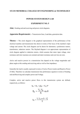
1. STANI MEMORIAL COLLEGE OF ENGINEERING & TECHNOLOGY
POWER SYSTEM DESIGN LAB
EXPERIMENT NO. 5
Aim:- Sending end and receiving end power circle diagrams.
Apparatus Requirements: - Transmission lines, Load data, generation data.
Theory: - The circle diagram is the graphical representation of the performance of the
electrical machine and transmission line drawn in terms of the locus of the machine's input
voltage and current. The circle diagram can be drawn for alternators, synchronous motors,
transformers, induction motors. The Heyland diagram is an approximate representation of
circle diagram applied to induction motors, which assumes that stator input voltage, rotor
resistance and rotor reactance are constant and stator resistance and core loss are zero.
Active and reactive powers in a transmission line depend on the voltage magnitudes and
phase angles at the sending and receiving ends as well as line impedance.
Generally the load is usually expressed in terms of Active Power (watts) and Reactive Power
(VARs). Therefore we calculate transmission line performance equation in terms of Sending
end and Receiving end complex power and Voltage.
Complex, active and reactive power flows in this transmission system are defined,
respectively, as follows:
SR = PR + jQR = VR I*

2. Similarly For Receiving End:
Where VS and VR are the magnitudes (in RMS values) of sending and receiving end voltages,
respectively, while δ is the phase-shift between sending and receiving end voltages.
The equations for sending and receiving active power flows, PS and PR, are equal because the
system is assumed to be a lossless system. As it can be seen in Figure 5.1 the maximum
active power transfer occurs, for the given system, at a power or load angle δ
.
Maximum power occurs at a different angle if the transmission losses are included. The
system is stable or unstable depending on whether the derivative dP/dδis positive or
negative. The steady state limit is reached when the derivative is zero.
In practice, a transmission system is never allowed to operate close to its steady state limit, as
certain margin must be left in power transfer in order for the system to be able to handle
disturbances such as load changes, faults, and switching operations. As can be seen in Figure
5.2 the intersection between a load line representing sending end mechanical (turbine) power
and the electric load demand line defines the steady state value f δ; a small increase in
mechanical power at the sending end increases the angle.
For an angle above 900, increased demand results in less power transfer, which accelerates
the generator, and further increases the angle, making the system unstable; on the left side
intersection, however, the increased angle increases the electric power to match the
increased mechanical power. In determining an appropriate margin for the load angle , the
concepts of dynamic or small signal stability and transient or large signal stability are often
used. By the IEEE definition, dynamic stability is the ability of the power system to maintain
synchronism under small disturbance, whereas transient stability is the ability of a power
system to maintain synchronism when subjected to a severe transient disturbance such as a
fault or loss of generation. Typical power transfers correspond to power angles below 300; to
ensure steady state rotor angle stability, the angles across the transmission system are usually
kept below 45.
Circuit Diagram:-
Fig 5.1 Model for calculation of real and reactive power flow

3. Fig 5.2 Power Angle Curve
Precautions:1. Do the calculations carefully.
2. Keep distance from live wire and electrical equipments.
Procedure:-
Observation Table:-
Calculation:-
Result: - We have successfully studied and draw Sending end and receiving end power
circle diagrams.

4. Viva- Voice Questions:Ques. 1 On which factor Active and reactive powers in a transmission line depend?
Ques. 2 What is dynamic stability?
Ques. 3 what is transient stability

5. Viva- Voice Answers:Ans. 1 Active and reactive powers in a transmission line depend on the voltage magnitudes
and phase angles at the sending and receiving ends as well as line impedance.
Ans. 2 Dynamic stability is the ability of the power system to maintain synchronism under
small disturbance.
Ans. 3 Transient stability is the ability of a power system to maintain synchronism when
subjected to a severe transient disturbance such as a fault or loss of generation.