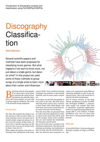
1. Visualization of discography analysis and
classification using PyCOMPSs/COMPSs
Discography
Classifica-
tion
Sofia Kypraiou
Several scientific papers and
methods have been proposed for
classifying music genres. But what
happens if we want to know more, not
just about a single genre, but about
an artist? In this project we used
some of these methods to group
songs of a single artist to learn more
about their career and influences.
B
eginning with the discography
of an artist with a long career,
we analyzed the songs extract-
ing features that describe them.
Then, after some analysis, we were able
to group songs by similarity. The result
is the beautiful image displayed!
Introduction
The idea that inspired the project was
the interest to find out more about an
artist and their career. Our goal was to
classify similar songs into groups in or-
der to see the variety of their music. Or
if you have a specific song that you like
from an artist, you can see similar works
by them. Cool, isn’t it?
What makes the project even more in-
teresting is the combination of the many
science fields. From machine learning
techniques and statistics to data mining
methods, and of course super comput-
ers.
As an input, we used the discography of
one artist at the time. We tried artists
with long music careers (U2), variation
in their music style (Pink Floyd), and
with many active years in both their mu-
sic career and style (David Bowie).
Then the music files are processed from
an audio extraction application in order
to extract some values that will be used
for the analysis. Some of the variables
that are used include the bandwidth,
the frequency and the pitch.
But not all of this data is needed in the
following computations. The data needs
cleaning, processing, and analyzing so
that we keep only the useful features.
After the data has been analyzed, it is
ready to be categorized using different
clustering methods in order to get the
optimal result. This is the result that is
used for the final visualization.
And of course, because of the large
dataset, parallelism is needed. The BSC
has developed COMPSs, a program-
ming model and runtime that aims
to parallelize sequential applications
written in sequential programming lan-
guages (like C, Java, Python). It makes
parallelism easy even for those that
don’t have a strong programming back-
ground.
Methods
As described before, the processing goes
through a number of stages, as follow-
ing:

2. Figure 1: The stages until the final result
Audio extraction
The audio extraction is used to get au-
dio feature sets that are evaluated in
their ability to differentiate. The fea-
ture sets include low-level signal proper-
ties, mel-frequency spectral coefficients
(MFCC). Low-level signal parameters re-
fer to a physical description of a song.
MFCC is commonly used in voice recog-
nition and is based on human hearing
perceptions. At the end, each song is
described with 72 features.
Data Analysis
Not all this information is useful and
by the end, only a small percentage of
them contributes to the final result. We
use Principal component analysis (PCA),
a statistical procedure used to empha-
size variation and bring out strong pat-
terns in a dataset, meaning that if a fea-
ture’s value doesn’t change a lot, then
it’s not useful.
By keeping 99% of the original infor-
mation, sometimes we would end up
having only 2(!) useful features.
Figure 2: Clustering of David Bowie’s discogra-
phy using K means (2 features after the PCA).
Clustering
Now that our data is pretty, clean
and tidy, we move to clustering. Clus-
ter analysis combines data mining and
machine learning. What we try to do is
group similar songs. Songs in the same
group (called a cluster) are more simi-
lar to each other than to those in other
groups.
So how do we choose which songs be-
long together? Well, there are many
methods that we used for this, each of
them producing different but compara-
ble results.
But we don’t know how many groups
there should be! How do we know
which is the best number of clusters?
Science is here to save the day, using a
metric called silhouette width that indi-
cates how well the clusters are formed.
Silhouette width has a range [-1,1], and
a value close to one means that the
items within each group are alike, and
that the groups are well separated.
Table 1: Clustering methods for Pink Floyd
Clustering
Method
Number of
clusters
Silhouette
width
Hierarchical 4 0.0927
Spectral 57 0.1975
KMeans 89 0.6208
DBSACN 2 0.4161
Propagation 116 1.0
But at the end, all this is just mathemat-
ics. Clustering methods lack intuition
and therefore human inspection is nec-
essary in the formation and determina-
tion of clusters. We need this in order to
gain an understanding of not only what
the data represents but also what the
cluster represents and what it intends
to achieve.
Vizualization
We understand the data better when
we see it. The data is brought to life us-
ing web technologies like HTML, CSS
and javascript library D3, producing dy-
namic, interactive data visualizations in
web browsers. The vizualization is the
result of the cluster analysis, using a de-
fault coloring, but also giving the user
the possibility of defining their own clus-
ters.
PyCOMPSs
For the purpose of performance, as
well as benefiting from the potential
of MareNostrum, Barcelona’s supercom-
puter, we used PyCOMPSs to parallelize
the audio extraction stage. Although in
our case it was not necessary due to
the small number of songs per artist,
PyCOMPSs could also be used in the
PCA and clustering stages. Songs are
separated in chunks, and each one of
them is assigned to a node in the su-
percomputer. Below is the graph of the
execution:
Figure 3: Graph of the execution. The blue
nodes indicate the tasks whilst the reds demon-
strate where synchronization was needed
Results
It is interesting to see which features
were useful at the end for the compu-
tations. From the data analysis (PCA
method), keeping the 99% of the useful
variables, we saw that only the MFCC
features were contributing to the calcu-
lations.
Our first attempt with the clustering
methods didn’t turn out as expected. As
you can see from Figure 2, the clusters
are so merged together with one being
into the other, and it’s very hard to dis-
tinguish them.
From table 1, the silhouette width
scores were low. A value lower than 0.3
means there is no structure in the data,

3. while something between 0.3 and 0.5
means there might be some structure.
Another interesting part was that it was
almost impossible to cluster Pink Floyd’s
discography. The graph 4 shows that al-
though we were able to group U2 songs
into 3 categories fairlyin easily, for Pink
Floyd it gives very poor results.
Figure 4: Best number of clusters for U2
(top) and Pink Floyd (bottom). Values below
0 indicate that the songs are wrongly classified.
Since that method didn’t work, we tried
taking samples for each song. The sam-
ples were taken at 0, 30, 60, 90, 120
seconds of the song. After running the
hierarchical clustering on this data, all
the introductions were put in one group,
an indication that our clusters worked
well.
Figure 5: U2 discography with 5 samples
per song. With the blue are all the
introductions
For the final vizualization, we used the
hierarchical clustering, and specifically
the dendrogram that it offers. For better
optical results, we used a polar dendro-
gram.
Figure 6: David Bowie discography.
Top: default coloring of the clusters
Bottom: user-defined clusters
At the bottom of the circle displayed are
all the studio album covers. On hover,
their songs are revealed in the dendro-
gram, making it easier for the user to
recognize them.
Figure 7: Pink Floyd discography.
Viewing songs of the ’Wall’ (1979)
The interactive dendrogam, along with
the discographies of U2, David Bowie
and Pink Floyd, can be found here.
Conclusion and further work
We used these stages and methods to
discover more about the artist’s mu-
sic career. The fact that we didn’t get
the expected results from the cluster-
ing means that MFCC features, although
suited for genre classification, are not
suitable for clustering songs of the same
artists (in the same genre).
Also, it is interesting that whilst U2 and
David Bowie songs could be grouped in
3 to 6 clusters, it was almost impossible
to group Pink Floyd songs.
One extension can be the recommenda-
tion of similar songs of the same artist.
It can be used in a variety of applica-
tions, like recommendation of top-N
songs of this artists, or in virtual dj pro-
grams.
References
1
Jeroen Breebaart, Martin McKinne Fea-
tures for Audio Classification 2003.
2
Lindasalwa Muda, Mumtaj Begam and
I. Elamvazuth Voice Recognition Algo-
rithms using Mel Frequency Cepstral
Coefficient (MFCC) and Dynamic Time
Warping (DTW) Techniques 2010
Acknowledgements
I would like to thank my mentor,
Fernando Cucchietti, for his guidance
through the project and for providing
the vizualizations along with Guillermo
Martin, the artist and Diana Fernanda
Velez García for the the graphic design.
Also Rosa Badia and Daniele Lezzi for
their support with PyCOMPSs. and last
but not least, Carlos Carrasco Jimenez
for the project and knowledge in ma-
chine learning, statistics, data analysis
and data mining.
PRACE SoHPCProject Title
Visualization data pipeline in
PyCOMPSs/COMPSs
PRACE SoHPCSite
Barcelona Supercomputing Center
(BCS-CNS), Spain
PRACE SoHPCAuthors
Sofia Kypraiou, [National and
Kapodistrian University of Athens,]
Greece
PRACE SoHPCMentor
Fernando Cucchietti, BSC, Spain Sofia Kypraiou
PRACE SoHPCContact
Fernando, Cucchietti, BSC
E-mail: fernando.cucchietti@bsc.es
PRACE SoHPCSoftware applied
Python, COMPSs/PyCOMPSs, D3.js
PRACE SoHPCMore Information
Music project COMPSs/PyCOMPSs, D3 JavaScript
library
PRACE SoHPCProject ID
1601